Quantification of magnetic nanoparticles by compensating for multiple environment changes simultaneously
Yipeng
Shi
 *a,
Dhrubo
Jyoti
b,
Scott W.
Gordon-Wylie
b and
John B.
Weaver
*abcd
aDepartment of Physics & Astronomy, Dartmouth College, Hanover, NH 03755, USA. E-mail: John.B.Weaver@hitchcock.org
bDartmouth-Hitchcock Medical Center, Lebanon, NH 03756, USA
cDepartment of Radiology, Geisel School of Medicine at Dartmouth College, Hanover, NH 03755, USA
dThayer School of Engineering, Dartmouth College, Hanover, NH 03755, USA
First published on 27th November 2019
Abstract
The quantification of magnetic nanoparticles is important for many applications, especially for in vivo biosensing. The magnetization harmonics used in spectroscopy of magnetic nanoparticles can be used to estimate nanoparticle number or weight. However, other effects such as temperature or relaxation time change can also influence the nanoparticle magnetization. Therefore, it is necessary to compensate for these factors when estimating the amount of magnetic nanoparticles. This paper shows through simulation that a two-dimensional scaling method can be used to improve the accuracy of nanoparticle quantification, especially when multiple effects are present which can influence the nanoparticle magnetization. Finally, an experiment was performed on a Magnetic Spectroscopy of Brownian motion (MSB) apparatus to demonstrate this method, and nanoparticle weight was determined with a mean error of 1.3 ng (1.81%).
1. Introduction
Magnetic nanoparticles (NPs) have been used in a range of applications, like biosensing involving protein binding,1 magnetic particle imaging,2 drug delivery1 and thermal therapy.3 For many of these applications, it is important to accurately monitor the number of particles.4 The magnetization from NPs is directly proportional to the NPs weight. However, the NPs magnetization is also affected by microenvironment effects including temperature, viscosity and bound state.Magnetic Spectroscopy of Brownian motion (MSB) has shown great promise in measuring these microenvironment effects.5–9 Multiple parameters can change the NPs harmonics simultaneously, and that complicates measurement of individual factors, especially in vivo. For example, to measure protein binding, the particle relaxation is affected by bound state, but also by the temperature. The two can have different effects on the NP harmonics even when the relaxation time changes the same amount.
The NPs weight can be estimated by compensating for the change in relaxation time.4 In this paper, we demonstrate that change in multiple microenvironment parameters can be compensated simultaneously to obtain more accurate estimates of the NP weight or number.
2. Methods
2.1 Theoretical basis
The magnetization, M, from an ensemble of magnetic NPs in a sinusoidal applied field can be described10 by two dimensionless variables using the Buckingham Pi Theorem and dimensional analysis. The dimensionless variables give scaling relationships between relaxation time and applied magnetic field frequency and between temperature and applied magnetic field amplitude. This allows the estimation of relaxation time and temperature change.11 The harmonics are directly proportional to the number of NPs present after correcting the changes in relaxation time and in temperature.The magnetization, M, of a given concentration ρ of NPs can been described10 using the two dimensionless variables as:
 | (1) |
The dependence of magnetization on the product of frequency and relaxation time means scaling frequency produces the same effect as scaling the relaxation time, enabling relaxation time measurement. Similarly, temperature can be measured by scaling magnetic field. The ratio of magnetization harmonics is used because it is independent of both the concentration of NPs and the coil geometry.5 Typically, we use the ratio of the second non-zero magnetic harmonic to the first non-zero magnetic harmonic. These first two harmonics tend to have the largest amplitudes hence yield best signal-to-noise. For a perpendicular geometry (pickup coil perpendicular to drive coil), this is the ratio of the fourth harmonic to the second harmonic,  .
.
The relaxation time and temperature can be measured by estimating scaling factors ε1 and ε2 to minimize  , where Ru is the harmonic ratio of the unknown state and Rr is of the reference state. The resulting scaling factors are the ratios of relaxation times τu/τr and temperatures Tr/Tu between the unknown and reference state. Similarly, the harmonic phase angles with respect to the driving field can also be used to estimate these scaling factors, and the combination of the harmonic ratio and phase angles has been shown to improve the accuracy of the temperature and relaxation measurement.10
The magnetization from the reference state at the scaled frequency ε1ω and magnetic field amplitude ε2H only differs from the unknown state at ω and H by the NP density. The magnetization and its corresponding nth order harmonics Fn are proportional to the NP concentration if the NP sample is dilute and particle interaction can be ignored. Therefore, the NPs density of the unknown state can be calculated by the ratio of the scaled harmonics:
| ρu = ρrFnu(ω, H)/Fnr(ε1ω, ε2H) | (2) |
In which ρu, ρr are the NPs density, and Fnu, Fnr are the nth harmonics in the unknown state and reference state, respectively.
2.2 Numerical methods
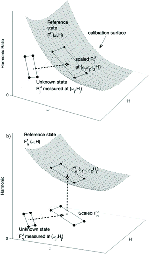
This method of estimating the NPs weight is illustrated in Fig. 1. The magnetization harmonics of NPs in the reference state are measured at a range of frequencies ω and magnetic field B. The ratio of harmonics Rr(ω, H) at the reference state forms the calibration surface in the 3D space with frequency ω and magnetic field B as the two independent variable axes. Harmonics of NPs at an unknown state and concentration are then measured at several frequencies ωj and magnetic field amplitudes Hj, resulting in the corresponding ratio of harmonics at the unknown state Rju, j = 1, 2,⋯n (n ≥ 2). The two scaling factors ε1 and ε2, representing the relative change in relaxation time and temperature, satisfy that ratio of harmonics at the scaled frequency and magnetic field amplitude (ε1ωj, ε2Hj) equals that of the unknown state at (ωj, Hj). Geometrically, this means the scaled ratio of harmonics of the unknown state, with data points of (ε1ωj, ε2Hj, Rju) j = 1, 2⋯n, fall onto the calibration surface.The two scaling factors can be calculated by interpolating the calibration surface at (ε1ωj, ε2Hj), and minimize the squared error  . A grid search method was used by calculating g with a range of values for both ε1 and ε2 and choosing the scaling factors which minimized squared error.
The relative density change can be calculated using Fnr, the harmonic from the reference state interpolated at the scaled frequency ε1ω and magnetic field amplitude ε2H, and Fnu, the harmonic from the unknown state at ω and H. A least squares estimate was made to calculate the NPs density at the unknown state, since multiple frequencies and magnetic amplitudes were measured for the unknown state.
2.3 Simulation methods
A stochastic simulation has been used to demonstrate the process of estimating the number of NPs by compensating for the change in both temperature and relaxation time. The full stochastic Langevin equation governing rotational dynamics of a magnetic Brownian particle suspended in fluid and placed in a magnetic field is:12 | (3) |
2.4 Experimental methods
Two sets of samples with iron weight of approximately 40 μg, 60 μg, 80 μg and 100 μg were prepared using Micromod BNF starch iron oxide NPs (average 110 nm hydrodynamic diameter). Glycerol was added to one set of samples to change relaxation time independent of temperature. PBS was then added to all the samples to equalize the volumes, so that the pickup coil fill factor is the same for all samples. The total volume of each sample was chosen to be 60 μL. The exact quantities of iron and glycerol in each sample were calculated from the measured weights on an electronic balance (Mettler Toledo, Model ML203E).The temperature of the samples was controlled by a water bath which runs through the MSB spectrometer and around the sample. The water bath was set to three different temperatures of 35 °C, 40 °C and 45 °C. The exact stable temperature of the sample was measured before the experiment using a thermometer. The relaxation time of the sample was thus changed by both the temperature and glycerol concentration.
For each of these three temperatures, the DC field was set to 0.8 mT, 1 mT and 1.2 mT by physically moving the pair of strong Neodymium magnets. The AC field was set to 8.0 mT, 10 mT and 12 mT respectively, maintaining the ratio of DC to AC fields. For each of these three field strengths at each of these three temperatures, the harmonics of the eight samples were measured using the MSB instrument at each of the 10 resonant frequencies: 603.1 Hz, 697.6 Hz, 817.9 Hz, 958.6 Hz, 1038.4 Hz, 1134.2 Hz, 1219.0 Hz, 1321.6 Hz, 1445.0 Hz, and 1595.0 Hz. The resonant frequencies were chosen by connecting various capacitors in series with the coil. The capacitors were chosen such that the resonant frequencies are roughly equally spaced over the entire range.
All samples were frigerated while not being measured. Just prior to measurement, the sample was placed in a dry bath for about 10 minutes and warmed to the target temperature, while waiting for the current sample to finish measuring. The 40 μg NP sample with glycerol were measured at temperature 35 °C as the reference sample. For this combination, the measurements were taken for 1.4, 1.15, 1.1, 1.0, 0.9 and 0.8 mT DC field, while maintaining the DC field to AC field ratio of 0.1.
The MSB spectrometer was a perpendicular geometry.13 A sinusoidal voltage signal was generated by a phase-locked amplifier (Zurich Instruments model HF2LI). This signal was amplified by an audio power amplifier (QSC model PL 236). This amplified signal was used to drive the coil at resonance frequencies to produce the applied field. The resonant frequency of the coil was varied by placing different capacitors in series with the coil. The various capacitors were switched on and off using a relay interface device (USB-ERB24, Measurement Computing). The signal from the NPs was first amplified by a preamplifier and then measured by the lock-in amplifier. The lock-in amplifier analyses the signal and measures the amplitude and phase of each harmonic with respect to the driving field.
3. Results and discussion
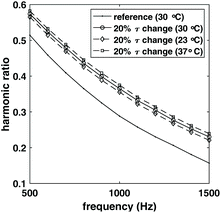
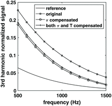
To demonstrate the complication caused by temperature change and the benefit of compensating for both relaxation time and temperature in estimating the number of NPs, a reference sample of 106 NPs was simulated first at 30 °C, 2 mPas viscosity. Three other samples with 3 × 10⁶ NPs with the same relaxation time, but different temperatures were simulated. The simulation was done for frequency between 500 Hz and 1500 Hz, and magnetic field amplitudes between 5 mT and 15 mT. The resulting ratio of harmonics is shown in Fig. 2 (only the 10 mT data was shown for simplicity). The ratio of harmonics were different for these three samples, even though the relaxation time change relative to the reference sample was the same. Since the ratio of harmonics are different, estimation of NPs weight based only on relaxation change would not be correct which shows that simply compensating for the effect of relaxation time would result in an error in the estimation of NPs weight.To further demonstrate the effect of compensating for both relaxation time change and temperature change, the third harmonics of the reference sample and target sample with 20% relaxation time change relative to the reference sample and 37 °C was shown in Fig. 3. The harmonics for the target sample was then scaled using the method described in section 2.2 to compensate for the change in relaxation time, and for both relaxation time and temperature change relative to the reference sample. The compensation for relaxation time resulted in a drop of the harmonics, and further compensating for temperature change increased the harmonics.
As mentioned in section 2.1 and eqn (2), the NP weight of the target sample is usually estimated by the relative change of harmonics relative to the reference sample. In this case, if no compensation was performed for the relaxation time and temperature change, it would result in an overestimation of NPs weight for the target sample; if only relaxation time change was compensated, it would result in an underestimation of the NPs weight for the target sample.
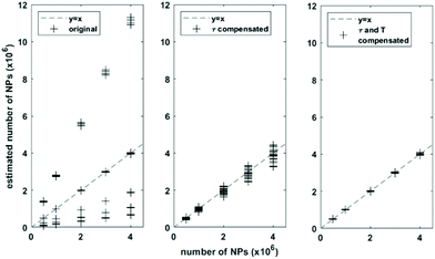
To further demonstrate the effect of compensating for the relaxation time and temperature change in estimating the NPs weight, a range of target NPs samples were simulated for temperature from 20 °C to 50 °C, viscosity from 1 mPas to 5 mPas. Each sample was simulated with alternating magnetic field with magnetic amplitudes from 5 mT to 15 mT, and frequencies from 500 Hz to 1500 Hz. Each unique temperature and viscosity state was simulated for four different NPs number. The number of NPs in each sample was then estimated by scaling the ratio of harmonics and harmonics following the method in section 2.2 by compensating relaxation time change and temperature change relative to the reference sample simulated earlier. The results were shown in Fig. 4. For comparison, the numbers of NPs for the target samples were also estimated by using the uncompensated harmonics and the scaled harmonics compensated for only relaxation time change.
With both relaxation time and temperature change, the estimation of NP number has a mean relative error of 0.55%. With compensation of only relaxation time, the relative error has mean of 7.38%. This error was large mainly because the temperature change of the target sample relative to the reference sample was as big as 20 °C, and compensating for temperature change is important for a correct estimation of NP weight in the case when the relative temperature change is large. Without any compensation of relaxation time and temperature change, the estimation gave the biggest error 77.66%, demonstrating the necessity of compensating for these micro environment change on the NPs dynamics.
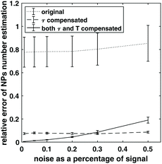
Adding experimental noise does not change the simulation results. The noise from instrumental and environmental sources contribute to the error. To demonstrate the effect of noise in the estimation of NP weight, random white noise was added to the simulated harmonics of the target samples of 3 × 10⁶ NPs with temperature and viscosity simulated previously, resulting in different noise to signal ratios for the harmonics. Number of NPs was estimated again for different noise levels, and the relative estimation error for NP number was calculated. The process was repeated 1000 times for each noise level, and mean and standard deviation of the relative error was shown in Fig. 5. When no compensation for relaxation and temperature change was performed, the estimation has the largest relative error. When both relaxation time and temperature were compensated for, the estimation error was lowest when the noise level was below 30% of the harmonic signal, and the relative error increased when the noise increased. It is worth noting that in the case when only relaxation time was compensated for, the relative error did not increase as much as the case when temperature change was also compensated for, and demonstrated a robustness by staying relatively low in the high noise range. This might be because compensating for both temperature and relaxation time requires interpolation in the two-dimensional surface mentioned in section 2.2, and can become unstable when the noise level is high. Plus, compensating for relaxation time does not require measuring the NPs sample at a range of magnetic field amplitude as mentioned in the method of section 2.2, which can be much faster. Therefore, it might be preferable to just compensate for relaxation time in some cases of estimating NP weight especially when there is a requirement for fast estimation and temperature change is not huge between the target and reference sample.
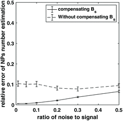
In addition, NPs number/weight estimation was simulated for a perpendicular MSB device.13 An additional perpendicular magnetic field directs the magnetization into the plane perpendicular to the alternating field helping to decouple the alternating field from the magnetization, that is, there is lower feed-through signal. The lower order harmonics can also be used, which usually have a bigger magnitude in signal, and, therefore, result in a higher signal to noise ratio for many applications. The estimation of NP number was simulated with both a fixed static magnetic field and a changing static magnetic which keeps the ratio of the two magnetic fields the same. Noise was added to the harmonics and repeated 1000 times, and the mean and standard deviation of the relative error was shown in Fig. 6. Keeping the ratio of the static to alternating fields constant achieved a lower error. Therefore, it is necessary to modify the experimental apparatus so that the static field amplitude can be changed to compensate the driving field when estimating the NPs weight using the perpendicular MSB apparatus.
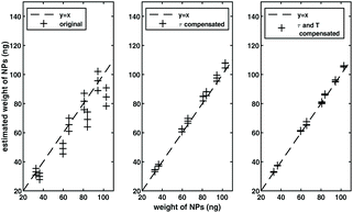
Finally, experiments were done with a perpendicular MSB device. The result is shown in Fig. 7. A range of samples described section 2.4 were measured with viscosity ranging from 0.656 mPas to 1.306 mPas, and temperature ranging from 30 °C to 40 °C. The NP weight of each sample was then estimated by scaling the ratio of harmonics and harmonics following the method in section 2.2 by compensating relaxation time change and temperature change relative to the reference sample. The sample with viscosity of 1.16 mPas and temperature of 35 °C was used as the reference. A mean estimated error of 1.3 ng was achieved. For comparison, when no compensation was used, the error in the estimated NP weight was 7.9 ng, and when only relaxation time was compensated for, the error in the mean weight was 2.6 ng.
In this experiment, by compensating for relaxation time, we achieved an improvement of more than factor of 3 in the NP weight estimation, and an additional factor of two when we compensated for both relaxation and temperature. It is worth noting that the two-dimensional scaling method does not require the particles to be mono-dispersed or mono-cored. This experiment has shown improvement in the NP weight estimation, even though the nanoparticles used in the experiment have a polydisperse size distribution. We expect that the improvements would be even larger if the range of temperatures and the range of relaxation times were larger. We also expect the compensation technique to yield better improvements if the experimental errors are made smaller, for example by controlling the DC field to AC field ratio more accurately through the improvement of experiment apparatus. Finally, the 2D-scaling method is time-consuming since a 2D range of parameters (of magnetic field and frequency) have to be measured experimentally. We can expect the 2D-scaling method to be preferable when a more accurate estimation is needed or when a big change happens in either temperature or relaxation time for NP sample.
4. Conclusions
We have demonstrated a method to estimate NP weight by compensating for both relaxation time and temperature changes simultaneously. NPs samples with different microenvironments were simulated, and the number of NPs in each sample was estimated. The lowest error was shown when both relaxation time and temperature change was compensated for compared to the situation with no compensation and only relaxation time change compensation. NP number estimation was also simulated for perpendicular MSB device, and the result showed that the static field needs to be scaled with the alternating field to achieve the best result. The two-dimensional scaling method was demonstrated experimentally using a perpendicular MSB device. The simulation results were confirmed: compensating for both relaxation time and temperature improved the NP weight estimate significantly.Conflicts of interest
The authors have no conflict to disclose.Acknowledgements
This research was supported by NIH Grant No. 1R21EB021456.References
- Y. W. Jun, J. W. Seo and J. Cheon, Acc. Chem. Res., 2008, 41, 179–189 CrossRef CAS PubMed.
- T. M. Buzug, G. Bringout, M. Erbe, K. Gräfe, M. Graeser, M. Grüttner, A. Halkola, T. F. Sattel, W. Tenner, H. Wojtczyk, J. Haegele, F. M. Vogt, J. Barkhausen and K. Lüdtke-Buzug, Z. Med. Phys., 2012, 22, 323–334 CrossRef PubMed.
- I. Brigger, C. Dubernet and P. Couvreur, Adv. Drug Delivery Rev., 2012, 64, 24–36 CrossRef.
- J. B. Weaver, X. Zhang, E. Kuehlert, S. Toraya-Brown, D. B. Reeves, I. M. Perreard and S. Fiering, Nanotechnology, 2013, 24, 325502 CrossRef PubMed.
- A. M. Rauwerdink, E. W. Hansen and J. B. Weaver, Phys. Med. Biol., 2009, 54, L51–L55 CrossRef PubMed.
- A. M. Rauwerdink and J. B. Weaver, J. Magn. Magn. Mater., 2010, 322, 609–613 CrossRef CAS.
- A. M. Rauwerdink and J. B. Weaver, Med. Phys., 2010, 37, 2587–2592 CrossRef PubMed.
- A. M. Rauwerdink and J. B. Weaver, Appl. Phys. Lett., 2010, 96, 033702 CrossRef.
- H. Khurshid, B. Friedman, B. Berwin, Y. Shi, D. B. Ness and J. B. Weaver, AIP Adv., 2017, 7, 056723 CrossRef PubMed.
- Y. Shi, H. Khurshid, D. B. Ness and J. B. Weaver, Phys. Med. Biol., 2017, 62, 8102–8115 CrossRef CAS PubMed.
- Y. Shi and J. B. Weaver, Med. Phys., 2019, 46, 4070–4076 CrossRef CAS PubMed.
- D. B. Reeves and J. B. Weaver, J. Appl. Phys., 2012, 112, 124311 CrossRef PubMed.
- D. B. Reeves and J. B. Weaver, J. Phys. D: Appl. Phys., 2014, 47, 045002 CrossRef PubMed.
| This journal is © The Royal Society of Chemistry 2020 |

