
 Open Access Article
 This Open Access Article is licensed under a Creative Commons Attribution-Non Commercial 3.0 Unported Licence
A new method for the SI-traceable quantification of element contents in solid samples using LA-ICP-MS†
Lena
Michaliszyn
 *a,
Tongxiang
Ren
b,
Anita
Röthke
a and
Olaf
Rienitz
a
*a,
Tongxiang
Ren
b,
Anita
Röthke
a and
Olaf
Rienitz
a
aPhysikalisch-Technische Bundesanstalt (PTB), Bundesallee 100, 38116 Braunschweig, Germany. E-mail: lena.michaliszyn@ptb.de
bNational Institute of Metrology (NIM), No. 18 Bei San Huan Dong Lu, Beijing 100029, P. R. China
First published on 28th November 2019
Abstract
The present work introduces a novel approach for the quantitative and SI-traceable analysis of element contents in solid materials with laser ablation inductively coupled plasma mass spectrometry (LA-ICP-MS). The laser ablation and the nebulizer system were connected to the torch using a y-piece. Several standard solutions having well-known element contents were introduced one after the other into the plasma simultaneously with the ablated material. In contrast to all other quantification methods the solid sample itself serves as the reference and the content of an analyte element was calculated based on the well-known content of the matrix element (like Si in a glass sample). Equations to describe the novel method were derived inspired by the standard addition method. To investigate the feasibility of the novel method, the contents of Pb and Rb were analysed in two commercially available standard reference materials (NIST SRM 610 and 612 glass samples). These solid samples were analysed together with solutions of different mass fractions of silicon as the reference element (R) and lead or rubidium as the analyte elements (A). The mass fractions of Pb and Rb measured in the two certified reference materials (CRMs) were equal to the certified values within the limits of their expanded uncertainties (U(wx(A)) with k = 2). Compared to other quantification methods, this new method enables SI-traceability for the measurement results without the need to employ preferably matrix-matched solid reference materials, which will be a great benefit for the application of laser ablation in general, especially considering the extreme lack of matrix-matched CRMs. The new method is best-suited to determine impurities in highly pure samples with a mass fraction of the matrix element close to 1 g g−1.
1. Introduction
In the 1980s a laser ablation (LA) system was coupled for the first time to an inductively coupled plasma mass spectrometer (ICP-MS). This opened the possibility to analyse a solid sample directly, without any dissolution process. Because there are fewer preparation steps the number of factors that influence the uncertainty could be reduced.1 Besides this, some typical disturbances of the ICP-MS analysis (especially of organic solutions), like signal suppressions by the matrix can be eliminated.2 Due to the fast measurements, less sample consumption, ease of application and the excellent detection limits,3 LA-ICP-MS has been established in many areas such as geology,4 medicine5 and biology, but also forensics and chemical analysis.4 For example, the healing process of trees, more specifically their bark, can be studied by observing the change in elemental composition over time by LA-ICP-MS so that co-factors of enzymes can be identified.6 Next to the biological usage, like the analysis of proteins by combination with gel electrophoretic techniques,7 the LA-ICP-MS measurements can be helpful in the clarification of car accidents by examining the traces of car paints.8 Furthermore, with this method it is possible to clarify the origin of antique objects, such as glasses, since the elemental composition depends on their provenance.9 Another field is depth-profiling, which becomes more important, among other applications, for coatings like in the semiconductor industry.10 The determination of the thickness of a layer with an LA-ICP-MS measurement is rapid and accurate up to, i.e., a single atomic layer.11 In contrast to these harder samples it is also possible to analyse some softer samples like tissue samples of liver or kidney, like Bauer et al. did for a better understanding of the mechanism of cisplatin as a chemotherapeutic drug.12A part of the development of LA-ICP-MS techniques is focused on making the measurements quantitative and improving these strategies. This challenge still persists, even though a lot of work has been done already to improve the technique to get a fully quantitative analysis.13
To date, there are several techniques which have been established as quantification strategies. One of them is internal standardisation. This is used for an improvement in accuracy and precision. It could compensate the effect of fluctuation in laser output energy and for example the variation in transport efficiency. An element contained in the same sample, with exactly known concentration and with a similar ablation behaviour should be used as the internal standard (IS) element.14 The matrix element is used as such in many cases because of its homogeneous distribution. This method can be used to normalise the signal intensity but it is not completely quantitative.15 Apart from that, an IS element can be added to the sample, like it is the case for an offline isotope dilution (ID) LA-ICP-MS analysis. Again, the homogeneous distribution of the IS element in the sample is essential. The sample will be mixed with the analyte element itself but in an isotopically enriched form (spike) and pressed to a pellet.16 Another opportunity is to dissolve the solid sample and add some spike solution. The homogenized mixture is deposited on a support material and evaporated to dryness.17 In the next step the so-prepared and spiked sample can be ablated and analysed.
The second technique is based on certified reference materials (CRMs). The prerequisite is that a matrix-matched standard material is available, because the fractionation process during the laser ablation as well as the ablation rate depends on and varies with the matrix18 resulting in matrix dependent sensitivities. There are some certified reference materials, but the major problem is their limited number as well as their sometimes insufficient homogeneity.9 So, for many solid samples there is no reference material commercially available.19 Even though some matrix-matched standard materials were self-made in laboratories, like O'Reilly et al. demonstrated it for biological tissue standards,20 some problems still remain. In the case of commercial CRMs the user has no influence on the element contents (you have to buy them as they are). Furthermore, it is extremely difficult and time consuming to prepare a reference material from scratch with the exact composition of the original sample by yourself.15 Wu et al. described an alternative way for this technique, namely standard addition with a CRM.21 For this purpose, they used a spiked CRM, made of apple leaves, for a standard calibration. Therefore, they dropped some standard solution on the sample. After 48 h adsorption time, the apple leaves were ground into a fine powder and pressed to a pellet. This standard was measured together with a leaf of Elsholtzia splendens as the sample. This method worked very well,21 but there is still the problem of an additionally required standard. Moreover, with this method there is a loss of the spatial resolution of the original sample, and it is unsuitable for some harder samples (like metals or stones) that are difficult or impossible to grind. Furthermore, Hoesl et al. presented the alternative to print some spiked inks onto the sample and the matrix-matched standards, respectively.22 With this method an internal standardisation and a calibration can take place in combination whereat a homogeneous printing is a main condition in this concept.22
The calibration with a matrix-matched standard shows a lot of different ways and offers a good opportunity for a quantitative analysis, but often a suitable CRM is not available and due to the complexity of the sample it is not possible to prepare a perfect reference material. The procedure also is time consuming.23
Another method is the online addition. This technique was used, for example, already in 1989.24 Through a glass y-piece the tube of the laser ablation and a spray chamber can be connected simultaneously to the torch. This system of parallel gas flows is required to make sure that the conditions are constant during the whole measurement time.15,24 Moreover, the plasma robustness is improved by adding a solution.25 With this setup standard solutions with different mass contents can be introduced simultaneously with an ablated material into the plasma so that the prevailing conditions are the same. With a concentration series of the standard solution a linear regression and with the resulting equation a quantification can be performed. However, this method still depends on matrix-matched standards to calculate the sensitivity ratio (wet plasma/dry plasma).26 One of the current developments is a calibration strategy based on online isotope dilution analysis (IDA) and LA-ICP-MS. For this, a spike solution is added into the gas flow after the LA sample cell so that the isotopic ratio of the element of interest is affected. The most critical part of this technique is to quantify the sample mass flow. For this purpose, the ablated material mass must be determined by assuming the density and amount of ablated sample per time. Although this method ends up in quantitative results with a good recovery, compared to results obtained with ICP-MS after a microwave-assisted digestion or with external calibration, this method still needs a reference standard which behaves very similar12 during the ablation, transport and ionization process.
In summary, there are already several different approaches and methods for quantitative LA-ICP-MS measurements. Each has its own advantages and disadvantages.15 However, the limited number of certified reference materials and the calibration with an additional sample runs like a thread through all these methods. Even if a reference material is added directly onto the sample, there is a loss in spatial resolution because of the necessary fine grinding to form a reasonably homogeneous pellet or it is hard to get a homogeneous distribution. Also, the mass flow of the ablated material is unknown and can only be estimated. It could change over time caused by the fact that the ablated material settles, e.g., on a valve within the laser system (online valve) and this can clog gradually.
To meet the increasing demands of new applications, it is important to develop new calibration and quantification methods as well as to improve existing ones.15 Thus, in this work a new quantification method using the sample itself as the matrix-matched reference material is introduced.
2. Mathematical background of the novel quantification approach
In this chapter, a brief overview of the necessary equations is given. For more details see the ESI.†A main problem of the previous methods for quantitative LA-ICP-MS measurements is the not exactly known mass flow of the ablated material and the ablated sample volume per time or per laser shot, respectively. The signal intensity measured with a mass spectrometer corresponds to the flow of analyte ions Ṅ with the constant of proportionality k. With the definition of the number of analyte ions N, the amount of substance n(jA) of one isotope as well as the mass fraction of the analyte element w(A), eqn (1) is obtained when assuming a constant flow of analyte ions.
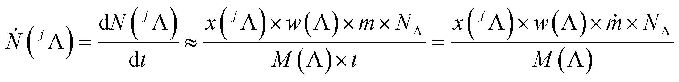 | (1) |
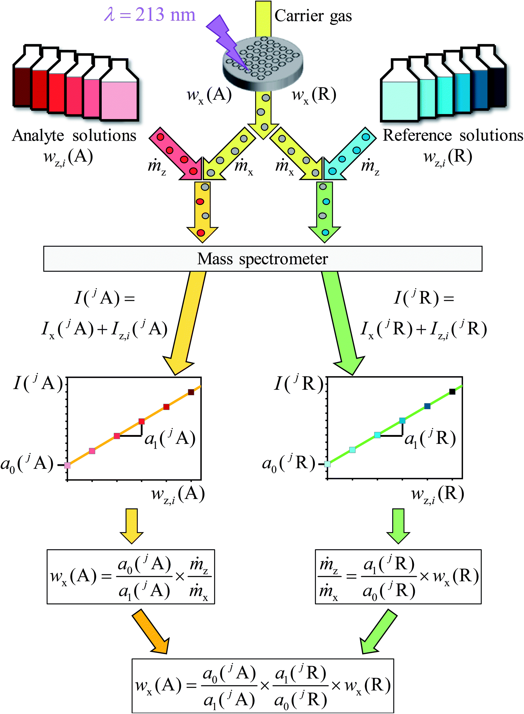
Like for the standard addition (online), for this technique a simultaneous injection of the ablated sample material (x) and a standard solution (z) into the plasma is required, which was realized by connecting the spray chamber and laser ablation to the torch via a y-piece (Fig. S1†). The measured intensity is the sum of the intensity resulting from the ablated sample Ix(jA) and the ith solution Iz,i(jA) belonging to a concentration series (in this work i = 0, 1, 2, … 5).
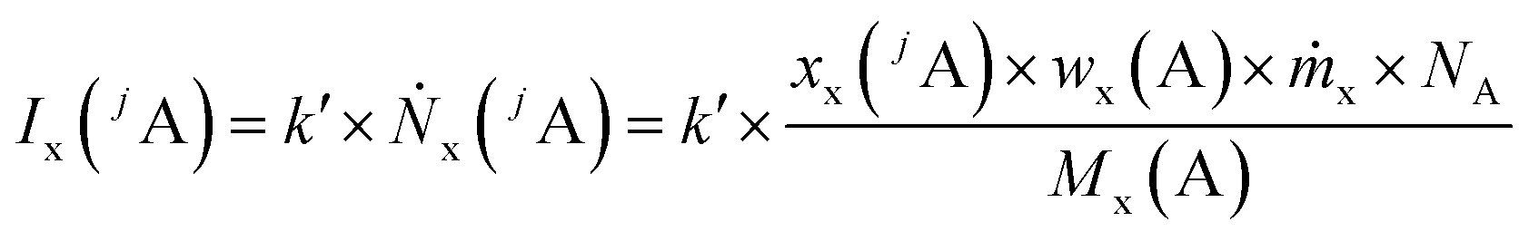 | (2) |
 | (3) |
By summing up the two equations above and assuming the same plasma conditions (k′ = k′′) as well as a constant mass flow and the same isotopic pattern for the solid sample and the solution (meaning xx(jA) = xz(jA), Mx(A) = Mz(A)), a linear equation results (eqn (4)). After subsequently measuring a certain number of solutions (i = 0, 1, 2, … 5) with different mass fractions wz,i(A) a regression line can be derived based on eqn (4) yielding the y-intercept a0 and the slope a1. Furthermore, by dividing the y-intercept by the slope, an equation for the mass fraction of the analyte element follows (eqn (6)).
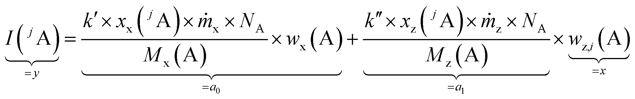 | (4) |
| y = a0 + a1 × x | (5) |
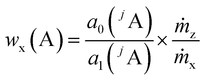 | (6) |
The mass flows are still unknown, but their ratio can be represented by the regression parameters and the mass fraction of the reference element (R). Therefore, R different from the analyte elements and with an exactly known mass fraction in the same sample must be measured as well. In highly pure samples the matrix element is often the best choice because of its homogeneous distribution and mass fraction w(R) ≈ 1 g g−1. This way, the sample itself acts as the (perfectly matrix-matched) reference material. With the known mass fraction wx(R) eqn (7) is obtained.
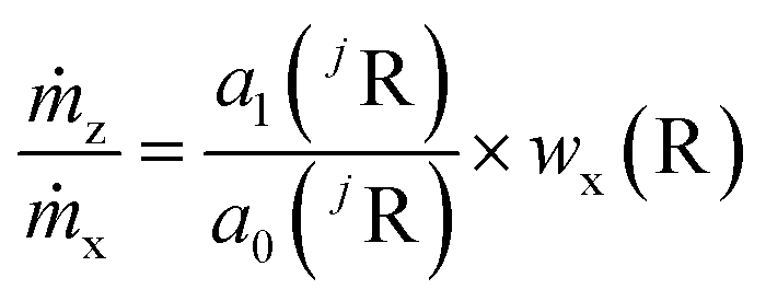 | (7) |
Assuming that all measurements, whether analyte or reference, will be done with the same sample and under the same plasma conditions, the analyte mass fraction wx(A) is expressed with eqn (8) which is obtained by combining eqn (6) and (7).
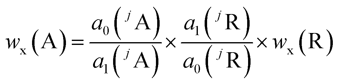 | (8) |
To obtain both regression lines, one measurement sequence with two parts is required. For both parts the background of the gas flows and the solvents of the solutions used should be measured as well as a concentration series of the analyte and the reference element. A schematic is shown in Fig. 2.
3. Experimental
To prove the concept of the novel method two different CRMs, namely NIST SRM 610 and NIST SRM 612, were used as samples. For these glass-based samples the contents of several analyte elements are certified. Lead (Pb) and rubidium (Rb) were chosen as the analyte elements because of very few interferences in the mass spectrometer and the availability of certified materials, required for the preparation of standard solutions. Moreover, these two elements with clearly different molar masses27 of M(Rb) ≈ 85 g mol−1 and M(Pb) ≈ 207 g mol−1 cover a wide range of the mass scale. Next to Pb and Rb as analytes, silicon (Si) was measured as the matrix element in the present study.In the first step, five solutions with different contents for each element were prepared in 0.15 mol kg−1 HNO3. The solution with the highest content was adjusted to yield twice the intensity of the signal gained by laser ablation of the solid sample. The respective element contents of Pb and Rb differ in the samples NIST SRM 610 and 612 by roughly one order of magnitude. Therefore, two different series of reference solutions for each analyte in both samples (NIST SRM 610 and 612) were necessary, in order to match the different contents of Pb and Rb. For the matrix element silicon one series of standard solutions was sufficient because of the almost same silicon content in both samples. The silicon solutions were prepared from Certipur® (NH4)SiF6 in H2O (Merck Millipore Corporation, Germany). The lead and the rubidium solutions were prepared from BAM-Y004 (BAM, Germany) and NIST SRM 984 (NIST, USA), respectively.
In the next step, for one measurement one analyte in one sample had to be chosen. To ensure the same plasma conditions for every measurement, one solution prepared of 0.15 mol kg−1 HNO3 and helium as a carrier gas of the laser ablation were introduced into the plasma during the entire measurement sequence (Fig. 1). Thus, a y-piece made of DURAN® borosilicate glass 3.3 (Fig. S1†) was used to connect the laser ablation and the spray chamber to the torch. A sequence with ablation spots and additional spots, so-called “blank spots”, was set up. During the analysis of a blank spot the laser was switched off, so that the background resulted from the LA carrier gas (helium), the MS sample gas (argon) as well as the solvent used as the blank solution. These blank measurements were used for the blank correction later on.
 | ||
| Fig. 1 Schematic of the measurement procedure. The laser ablated material transported by helium is introduced into the plasma. Further specific solutions are injected as well. First, solutions for the reference element (R) are added, afterwards standard solutions prepared of the analyte element (A). Because of the different mass fractions of the solutions and the linearity of the obtained intensities, two linear equations can be derived. The parameters of these equations are used to calculate the mass fraction of the analyte (wx(A)). | ||
After the first silicon blank spot the laser ablation was started (Fig. 1). The ablated material transported by helium was introduced into the plasma simultaneously with one solution. For the first ablation spot the blank solution was used, for the second spot the solution with the lowest content of silicon, for the third the solution with the next higher mass fraction of Si and so on. After finishing the analysis of the silicon solutions, a second blank spot was measured. Subsequently, the analysis of the chosen analyte was performed according to the same procedure. At this point two rows of laser ablation spots on the sample surface were finished. For compensation of the laser energy fluctuation and/or inhomogeneities, silicon as well as the analyte was measured three times, resulting in a sequence consisting of six spot-rows. The order of such a sequence with a total number of 48 spots, including the blank spots, is shown in Fig. 2.
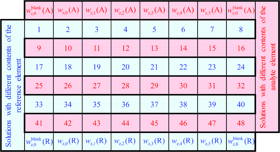 | ||
| Fig. 2 Schematic of one sequence. | ||
This figure shows the order of additions of the different solutions together with the ablated sample into the plasma and the blank spots where no ablation takes place, respectively. For one complete measurement 24 spots for the reference element R (in this case silicon) and 24 spots for the chosen analyte element A (in this case lead or rubidium, respectively) were used in which six blank spots per element were included. For all spots, except the blank spots, an ablation with identical parameters took place. All solutions were prepared from the same solvent wz,0 which was used as the blank solution and was added to the ablated material of every first ablation spot of a row.
In this work, the high-resolution inductively coupled plasma mass spectrometer Element XR combined with the UV laser NWR 213 was used. The operating parameters are listed in Tables 1 and 2. Every experiment to quantify one analyte in one sample was repeated three times. To protect the detector and to be able to operate in the same mode (in this case the analogue mode), the silicon isotope 30Si with the lowest abundance was chosen as the analyte isotope of the reference element. In contrast to the mass fraction of silicon, the mass fractions of lead and rubidium in the solid samples were quite low. In consequence the lead and rubidium isotopes with the highest natural abundance were monitored. Another reason is that 87Sr, which is present in both NIST samples, is an interference of the 87Rb (lower abundance) and cannot be separated in the Element XR mass spectrometer. Therefore, 30Si, 85Rb and 208Pb were chosen.
| Laser | NWR 213 (Electro Scientific Industries, USA) |
| Wavelength | 213 nm |
| Fluence | ∼21 J cm−2 |
| Repetition rate | 20 Hz |
| Spot size | 80 μm |
| Distance between two spot centres | 0.12 mm |
| Output energy | 80% |
| Ablation mode | Single spot |
| Carrier gas | 400 mL min−1 helium 5.0 (Linde group) |
| Dwell time pre-ablation | 3 s |
| Dwell time ablation | 19 s |
| Washout time | 110 s |
| Warmup time | 50 s |
| ICP-MS | Element XR (Thermo Fisher Scientific, Germany) |
| Rf power | 1195 W |
| Sampler and skimmer cone | Nickel (H skimmer) |
| Cool gas flow rate | 16 L min−1 argon 5.0 |
| Auxiliary gas flow rate | (0.60–0.80) L min−1 argon 5.0 |
| Sample gas flow rate | (0.950–0.980) L min−1 argon 5.0 |
| Detector mode | Analogue |
| Resolution | 4000 (medium) |
| Isotopes | 30Si, 85Rb, 208Pb |
| Sensitivity S | S(30Si) = 2.0 × 10⁵ s−1 (μg g−1)−1 |
| S(85Rb) = 2.0 × 10⁴ s−1 (μg g−1)−1 | |
| S(208Pb) = 2.7 × 10⁴ s−1 (μg g−1)−1 |
4. Calculation of mass fraction
The aim of this work was the development of a new method for quantitative LA-ICP-MS analyses which are traceable to the SI. To demonstrate the validity of this new concept, the mass fractions of lead and rubidium in NIST SRM 610 and 612 were analysed.One sequence contained 48 laser ablation spots. For every single spot 25 mass spectra were recorded. When the laser starts with the ablation process, a trigger is sent to the computer of the mass spectrometer which directly starts the measurements. But because of the distance the ablated material has to travel, from the ablation chamber through the transport tube into the plasma and furthermore the distance from the torch into the detector, an additional delay of approximately 7 s was caused (Fig. 3). Therefore, for every new measurement sequence it is necessary to define which spectra will be taken into account for the calculation of the result. Also, the section of the peak used to calculate the average had to be chosen carefully (Fig. 3), because of a slightly different mass offset on different days. Especially if measurements of a solution were compared with those of a laser ablation, a slight shift of the peaks was observed. The observation that the obtained intensities were not completely stable was caused by the fluctuating fluence (it differs in part by ±2 J cm−2). Additionally, a possible slight inhomogeneity in the sample could lead to small variations in intensities.
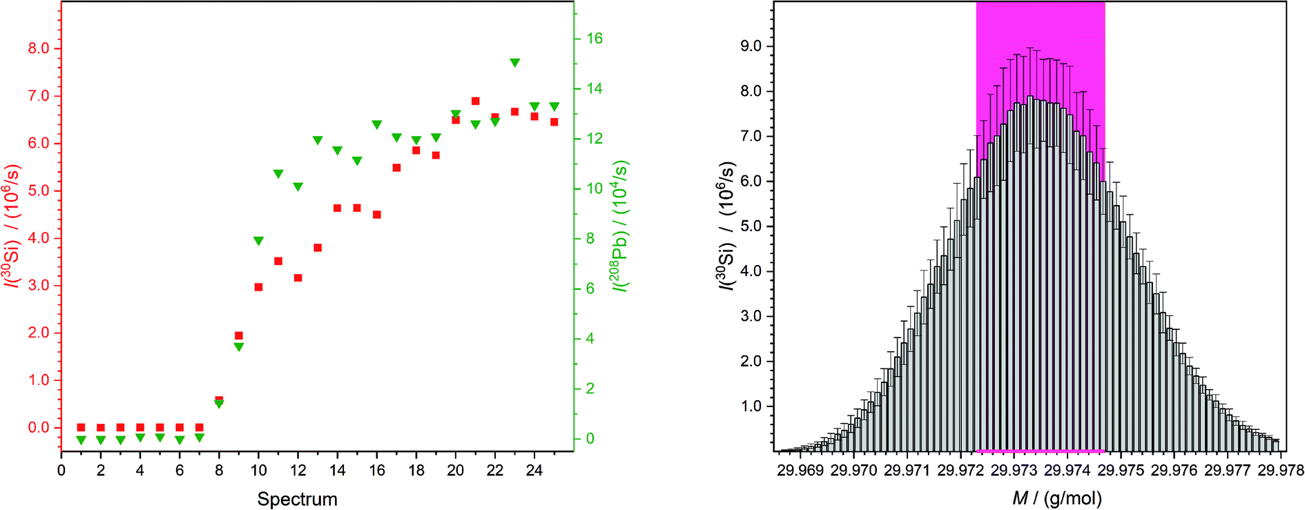 | ||
| Fig. 3 Both figures belong to the second “HNO3 spot” (wz,0) of the third measurement of the quantification of lead in NIST SRM 612. On the left-hand side exemplary intensity curves of a chosen mass for silicon (I(M = 29.973770 g mol−1),25 red squares) and one for lead (I(M = 207.976652 g mol−1),25 green triangles) are shown. This displays clearly the time which the material needs from being ablated to reach the detector as an ion. On the right-hand side the peak is shown which is a result of the determination of the average of spectra numbers 10 to 25 on the left-hand side (but for all detected masses). So, the mean obtained peak of silicon from NIST SRM 612 is displayed with the standard deviations. Next to this the values which are used to calculate the overall mean intensity for this spot is marked with a pink background. | ||
Subsequently, a blank correction was applied. For this purpose, the mean values of the signal intensities measured with the two blank solutions in a row (for example blank spot number 25 and 32 in Fig. 2) were subtracted from that of each ablation spot in the same row. By this calculation of mean intensities, for every measurement two graphics like Fig. 4 were obtained. From each regression line the associated y-intercepts a0 and slopes a1 were determined. These parameters were inserted in eqn (8). So, for the example given in Fig. 4, the parameters of the analyte a0(Pb) = 1.20 × 10⁵ s−1 and a1(Pb) = 2.22 × 10⁴ s−1 (ng g−1)−1 as well as of the reference a0(Si) = 5.99 × 10⁶ s−1 and a1(Si) = 1.34 × 10⁵ s−1 (μg g−1)−1 were used. The mass fraction of silicon oxide in both samples (SRMs) is given as 0.72 g g−1 SiO2,28 resulting in a mass fraction of silicon wx(Si) = 0.34 g g−1 in both materials. Using this value for wx(Si) and eqn (8), the mass fraction of the respective analyte wx(Pb) was obtained. For the mentioned example – the quantification of lead in SRM 612 – an analyte mass fraction of wx(Pb) ≈ 41 μg g−1 resulted.
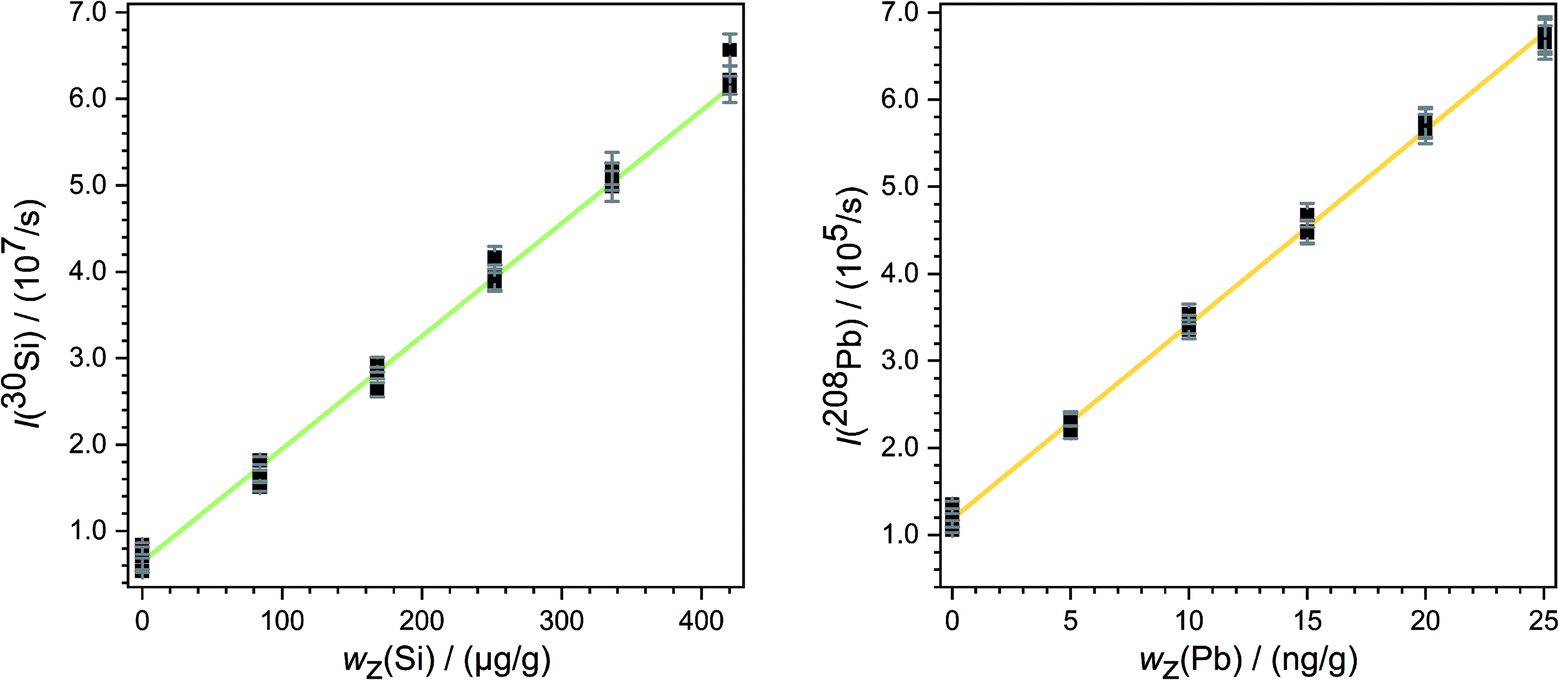 | ||
| Fig. 4 Mean intensities of 30Si (left) and 208Pb (right) in NIST SRM 612 (third measurement). The error bars denote the experimental standard uncertainties and the straight green and yellow lines show the linear regression. | ||
The continuous deposition of ablated material on a valve in the laser system leads to a loss of intensity. In particular, this is reflected by comparing the measurements carried out on different days (Fig. 5). Of course, day-dependent fluctuations also play into this effect. Here one example is shown but the graphics for all the other measurements are given in the ESI.† However, this effect has an impact on silicon as well as on lead or rubidium measurements. Due to the mathematical compensation, the results of the various measurements do not differ significantly from each other.
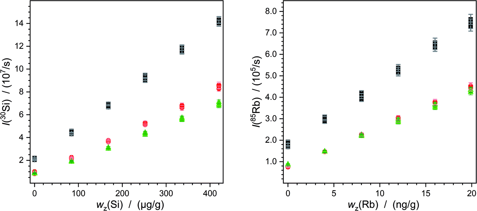 | ||
| Fig. 5 Mean intensities of 30Si (left) and 85Rb (right) as a result of the measurement with NIST SRM 612. The error bars denote the experimental standard uncertainties. The first sequence is represented by the black squares, the second sequence by the red circles and the last measurement sequence by the green triangles. One data point stands for the mean intensity of one laser ablation spot in addition to one standard solution. | ||
The software GUM Workbench29 was used for the calculation of the mass fractions with their corresponding expanded uncertainties according to the GUM (Guide to the Expression of Uncertainty in Measurement),30 taking into account the revised Type A evaluation according to GUM Supplement 1.31 The results of the single measurements are given in Table 3. All measurements show a reproducible behaviour.
| Sample | NIST SRM 610 | NIST SRM 612 | |||||||
|---|---|---|---|---|---|---|---|---|---|
| Analyte | Measurement | w x/μg g−1 | U/μg g−1 | U rel/% | Δ/% | w x/μg g−1 | U/μg g−1 | U rel/% | Δ/% |
| Pb | No. 1 | 402 | 82 | 20 | −6 | 38.4 | 5.5 | 14 | −0.4 |
| No. 2 | 413 | 76 | 18 | −3 | 43.9 | 7.8 | 18 | +14 | |
| No. 3 | 401 | 70 | 17 | −6 | 41.0 | 11.0 | 27 | +6 | |
| Mean | 405 | 76 | 19 | −5 | 41.1 | 8.4 | 21 | +7 | |
| Rb | No. 1 | 402 | 45 | 11 | −6 | 30.6 | 3.9 | 13 | −3 |
| No. 2 | 458 | 78 | 17 | +8 | 31.7 | 6.5 | 21 | +1 | |
| No. 3 | 420 | 100 | 24 | −1 | 31.2 | 5.9 | 19 | −1 | |
| Mean | 427 | 78 | 18 | +0.2 | 31.2 | 5.5 | 18 | −1 | |
The relative expanded uncertainty of a single measurement ranges from 10% to 30% which seems to be relatively large. This is caused by the fluctuation in laser output energy, variation of the composition of the sample and degraded material transportation out of the crater which becomes deeper and deeper. But on the other hand, the deviation of the three values among each other, obtained per analyte and sample, is equal to or lower than 7%. Within the scope of measurement uncertainties, it is not possible to distinguish between calculated and certified values. Fig. 6 displays this overlap of calculated and certified mass fractions clearly.
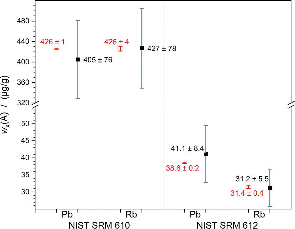 | ||
| Fig. 6 Measured mass fractions (black) of lead and rubidium in NIST SRM 610 and 612 compared to the certified values (red); error bars denoting the expanded uncertainties U with k = 2. | ||
The results of the quantifications of Rb (M = 85 g mol−1) and Pb (M = 207 g mol−1) show that the simultaneous introduction of the ablated sample and a reference solution, prepared of the chosen analyte, seems to open up the possibility to quantify elements over a wide mass range. With a maximum discrepancy of 7% the averages are very close to the certified values. This method is, even with an expanded uncertainty of about 20% (k = 2), a step forward as it enables straightforward uncertainty estimation and the establishment of SI-traceability. In the future, an optimisation of this new method would be meaningful for quantification of analytes with much lower content in the samples. Additionally, some parameters may be optimised to be able to work with smaller spot sizes. A better-known mass fraction of the matrix element will also improve the results, as its uncertainty directly impacts the result. This work lays the foundations for SI-traceable quantitative measurement without any need for a matrix-matched reference material for LA-ICP-MS.
The measurement results demonstrate the capability of the new method to reproduce the certified mass fractions of Rb and Pb in the NIST glass materials within their limits of uncertainties. Even though only the method presented here comprises a reasonable uncertainty, in order to assess the method, it is helpful to compare the results to those determined using already established quantitative methods. For example, more than ten years ago, Raith et al. published a paper in which various reference materials from similar matrices were used to calculate a calibration line. The deviations from the certified values were around 3% for SRM 610 (Rb and Pb) and in SRM 612 7% for Rb and 16% for Pb.32 In addition to the sample itself several solid reference materials, with similar matrices but different mass contents, were required for this approach.
Four years later, a study was published in which three normalisation factors for the calculation of the mass content in the solid sample were used. At first a concentration series of the analyte element containing a constant concentration of an internal standard is required. Subsequently, after obtaining the intensity of the analyte element in the ablated material, the corresponding concentration in solution (should be the same intensity) must be selected out of the calibration line. With this method it was possible to quantify Rb in SRM 612 very accurately (2% of the certified value). For lead the authors encountered some not specified problems: the result differs 35% from the certificate.33 The determined recovery of the results with respect to the certificate became worse with increasing mass of the analyte element. In our work, using the solid sample itself as the reference material, no significant dependence of the recovery on the element mass was observed (Pb in SRM 612: 7%).
In 2006, Kuhn et al. characterised the particle size in addition to the ICP-MS measurements. Using this information as well as the density of the sample and a reference material, it was possible to quantify the analyte element content. This so-called volume standardisation yielded a result very close to the certificate (1% for Pb in SRM 612).34 This method seems to be suitable, but besides the LA-ICP-MS a setup for the optical measurement is necessary and the density has to be determined, rendering the method technically demanding and error-prone. Table 4 summarizes the results discussed above compared to the results presented in this work. Even though the new method seems to be only a minor improvement in terms of recovery, it is the only one so far allowing for SI-traceable results accompanied by a reasonable measurement uncertainty.
5. Discussion and conclusion
In the last few years a lot of research was carried out in the field of laser ablation coupled to ICP-MS. During this time several techniques for a quantitative analysis were developed and established. All of them are characterized by their specific advantages and disadvantages. Because of the limited number of available CRMs and the difficulties of the online addition, the development of methods, not relying on matrix-matched solid reference materials and not requiring the knowledge of the mass of the ablated material, still helps to improve the acceptance of laser ablation coupled to ICP-MS as a quantitative method.Therefore, a novel quantitative technique for LA-ICP-MS measurements, which yields results traceable to the SI, was developed in this work. This method is based on the one hand on a simultaneous introduction of ablated solid sample and an aerosol of a standard solution into the plasma and on the other hand on the principle of standard addition. With this technique it is not necessary to determine the ablated volume or the mass flow. The most remarkable property of the novel approach/method is that for the first time the solid sample itself acts as the reference. This is a big advantage considering the finite number of reference materials. It could guarantee exactly the same sample ablation, transport and ionisation behaviour as well as exactly the same plasma conditions during the entire measurement sequence. Accordingly, one element of the sample has to be known very well. In the case of highly pure samples the matrix element itself is the best-suited choice but of course another element with well-known content can also be used. Thus, in the present work, standard glass materials (NIST SRM 610 and 612) were used with silicon as the reference element. Using this, lead and rubidium were quantified in both samples. The results are within the scope of their uncertainties very close to the certified value.
In one measurement it is possible to analyse one element in one sample. For this, silicon as well as the analyte was measured from the solid sample. As it takes place in a standard addition first the ablated material and a pure solvent were introduced into the plasma. In the next steps the concentration of the reference/analyte in the solution used was increased. After finishing the sequence and analysing the intensities, a linear regression was done for the silicon and the analyte measurement. The mass fraction can be calculated by using the parameters of this regression lines. The uncertainty from the mass content of the silicon, which was used as the reference element, was assumed and it affected the result directly. So, with a sample with a better-known mass content of the reference element, like it is the case for highly pure samples (wx(R) ≥ 99.9%), the results and their uncertainties will be much better.
The method presented has some disadvantages: the preparation of the series of reference and analyte element solutions is time-consuming, running a complete sequence takes approximately four hours, and the mass fraction (and its uncertainty) of the reference element must be well-known. In case the reference and analyte elements are compatible, solutions containing both elements can be prepared and measured, saving at least a certain amount of time. On the other hand, the method presented has some crucial advantages: the results are SI-traceable and comprise a realistic and reliable measurement uncertainty, enabling the comparability of the measurement results. In summary, the method presented is best-suited to determine impurities in highly pure samples with a mass fraction of the matrix element close to 1 g g−1 in all cases where comparable and accurate quantitative results are required irrespective of the necessary efforts.
Conflicts of interest
There are no conflicts to declare.Acknowledgements
The authors would like to thank all colleagues involved in this project. In particular, a big thank you to Axel Pramann and Janine Noordmann for the stimulating discussions, as well as to Reinhard Jährling. Furthermore, the authors would like to thank Carola Pape for her support.References
- A. L. Gray, Analyst, 1985, 110, 551–556 RSC.
- N. Vorapalawut, P. Pohl, B. Bouyssiere, J. Shiowatana and R. Lobinski, J. Anal. At. Spectrom., 2011, 26, 618–622 RSC.
- D. Günther, Anal. Bioanal. Chem., 2002, 372, 31–32 CrossRef PubMed.
- D. Günther and B. Hattendorf, Trends Anal. Chem., 2005, 24, 255–265 CrossRef.
- M. Resano, M. Aramendía, L. Rello, M. L. Calvo, S. Bérail and C. Pécheyran, J. Anal. At. Spectrom., 2013, 28, 98–106 RSC.
- M. Siebold, P. Leidich, M. Bertini, G. Deflorio, J. Feldmann, E. M. Krupp, E. Halmschlager and S. Woodward, Anal. Bioanal. Chem., 2012, 402, 3323–3331 CrossRef CAS PubMed.
- A. Raab, B. Pioselli, C. Munro, J. Thomas-Oates and J. Feldmann, Electrophoresis, 2009, 30, 303–314 CrossRef CAS PubMed.
- I. Deconinck, C. Latkoczy, D. Günther, F. Govaert and F. Vanhaecke, J. Anal. At. Spectrom., 2006, 21, 279–287 RSC.
- M. Bertini, A. Izmer, F. Vanhaecke and E. M. Krupp, J. Anal. At. Spectrom., 2013, 28, 77–91 RSC.
- J. Pisonero and D. Günther, Mass Spectrom. Rev., 2008, 27, 609–623 CrossRef CAS PubMed.
- B. Hattendorf, J. Pisonero, D. Günther and N. Bordel, Anal. Chem., 2012, 84, 8771–8776 CrossRef CAS PubMed.
- O. B. Bauer, C. Köppen, M. Sperling, H.-J. Schurek, G. Ciarimboli and U. Karst, Anal. Chem., 2018, 90, 7033–7039 CrossRef CAS PubMed.
- D. Pozebon, G. L. Scheffler, V. L. Dressler and M. A. G. Nunes, J. Anal. At. Spectrom., 2014, 29, 2204–2228 RSC.
- H. P. Longerich, D. Günther and S. E. Jackson, Anal. Bioanal. Chem., 1996, 355, 538–542 CrossRef CAS PubMed.
- D. Hare, C. Austin and P. Doble, Analyst, 2012, 137, 1527–1537 RSC.
- S. F. Boulyga, M. Tibi and K. G. Heumann, Anal. Bioanal. Chem., 2004, 378, 342–347 CrossRef CAS PubMed.
- P. Phukphatthanachai, J. Vogl, H. Traub, N. Jakubowski and U. Panne, J. Anal. At. Spectrom., 2018, 33, 1506–1517 RSC.
- R. Russo, Talanta, 2002, 57, 425–451 CrossRef CAS PubMed.
- D. Günther, R. Frischknecht, H.-J. Müschenborn and C. A. Heinrich, Fresenius. J. Anal. Chem., 1997, 359, 390–393 CrossRef.
- J. O'Reilly, D. Douglas, J. Braybrook, P.-W. So, E. Vergucht, J. Garrevoet, B. Vekemans, L. Vincze and H. Goenaga-Infante, J. Anal. At. Spectrom., 2014, 29, 1378–1384 RSC.
- B. Wu, Y. Chen and J. S. Becker, Anal. Chim. Acta, 2009, 633, 165–172 CrossRef CAS PubMed.
- S. Hoesl, B. Neumann, S. Techritz, M. Linscheid, F. Theuring, C. Scheler, N. Jakubowski and L. Mueller, J. Anal. At. Spectrom., 2014, 29, 1282–1291 RSC.
- M. Resano, E. García-Ruiz and F. Vanhaecke, Mass Spectrom. Rev., 2010, 29, 55–78 CAS.
- M. Thompson, S. Chenery and L. Brett, J. Anal. At. Spectrom., 1989, 4, 11–16 RSC.
- M. R. Flórez, M. Aramendía, M. Resano, A. C. Lapeña, L. Balcaen and F. Vanhaecke, J. Anal. At. Spectrom., 2013, 28, 1005–1015 RSC.
- D. Pozebon, V. L. Dressler, M. F. Mesko, A. Matusch and J. S. Becker, J. Anal. At. Spectrom., 2010, 25, 1739–1744 RSC.
- M. Wang, G. Audi, A. H. Wapstra, F. G. Kondev, M. MacCormick, X. Xu and B. Pfeiffer, Chin. Phys. C, 2012, 36, 1603–2014 CrossRef.
- (a) National Institute of Standards and Technology, Certificate of Analysis Standard Reference Material® 610, Trace Elements in Glass, Gaithersburg, 2012 Search PubMed; (b) National Institute of Standards and Technology, Certificate of Analysis Standard Reference Material® 612, Trace Elements in Glass, Gaithersburg, 2012 Search PubMed.
- R. Kessel, GUM Workbench Pro, Metrodata GmbH Search PubMed.
- Joint Committee for Guides in Metrology, Evaluation of measurement data — Supplement 1 to the “Guide to the expression of uncertainty in measurement” — Propagation of distributions using a Monte Carlo method, available at https://www.bipm.org/utils/common/documents/jcgm/JCGM_101_2008_E.pdf Search PubMed.
- Joint Committee for Guides in Metrology, Evaluation of measurement data — Guide to the expression of uncertainty in measurement, available at https://www.bipm.org/utils/common/documents/jcgm/JCGM_101_2008_E.pdf Search PubMed.
- A. Raith, J. Godfrey and R. C. Hutton, Fresenius. J. Anal. Chem., 1996, 354, 163–168 CrossRef CAS.
- M. Bi, M. A. Ruiz, B. W. Smith and J. D. Winefordner, Appl. Spectrosc., 2016, 54, 639–644 CrossRef.
- H.-R. Kuhn and D. Günther, J. Anal. At. Spectrom., 2006, 21, 1209–1213 RSC.
Footnote |
| † Electronic supplementary information (ESI) available. See DOI: 10.1039/c9ja00296k |
| This journal is © The Royal Society of Chemistry 2020 |