On-surface chemical reactions characterised by ultra-high resolution scanning probe microscopy

Abstract

In the last decade it has become possible to resolve the geometric structure of organic molecules with intramolecular resolution using high resolution scanning probe microscopy (SPM), and specifically using the subset of SPM known as noncontact atomic force microscopy (ncAFM). In world leading groups it has become routine not only to perform sub-molecular imaging of the chemical, electronic, and electrostatic properties of single molecules, but also to use this technique to track complex on-surface chemical reactions, investigate novel reaction products, and even synthesise new molecular structures one bond at a time. These developments represent the cutting edge of characterisation at the single chemical bond level, and have revolutionised our understanding of surface-based chemical processes.

---

Adam Sweetman

Adam Sweetman is a Royal Society University Research Fellow at the University of Leeds, UK. He obtained his PhD from the University of Nottingham in 2010, and subsequently held postdoctoral research positions at the same institute. In 2012 he held a JSPS Short term fellowship at NIMS in Tsukuba, Japan, and from 2014–2017 was awarded a Leverhulme Early Career Fellowship at the University of Nottingham. Since 2018 he has held his current position at the University of Leeds, where his research interests are focused on understanding the nature of interatomic and intermolecular forces via ultra-high-resolution scanning probe microscopy techniques.

Neil R. Champness

Neil R. Champness is the Professor of Chemical Nanoscience at the University of Nottingham, UK. After completing his PhD at the University of Southampton, UK, with Bill Levason he moved to Nottingham in 1995 reaching his current position in 2004. His research spans chemical nanoscience and all aspects of molecular organization, including surface supramolecular assembly and supramolecular chemistry in the solid-state via crystal engineering.

Alex Saywell

Alex Saywell is a Royal Society University Research Fellow at the University of Nottingham, UK. After obtaining his PhD in 2010 he moved to the Fritz Haber Institute of the Max Planck Society in Berlin as a postdoctoral researcher before returning to Nottingham in 2015 to hold Marie Curie IEF and Nottingham Research Fellowships, achieving his current position in 2018. His research focuses on the interdisciplinary area of nanoscience, studying surface confined molecular reactions and interactions via scanning probe microscopy characterisation techniques.

---

Key learning points

• What do scanning probe microscopes measure? – Providing background and context to the ncAFM technique.

• How do we observe molecule–substrate systems? – Experimental prerequisites for ncAFM.

• What does the ‘image’ show? – Origin of contrast in images and its interpretation.

• How does an on-surface chemical reaction progress? – Imaging of intramolecular bonds.

• Is seeing believing? – Interpretation of ‘intermolecular bonds’ and potential for imaging artefacts.

1 Introduction

Scanning probe microscopy (SPM) is a technique that facilitates the characterisation of single molecules and assemblies of molecules, confined to a supporting substrate, on the sub-molecular level. The defining characteristic of all variants of SPM is, as the name suggests, the use of a ‘probe’ to measure a specific probe–sample interaction over a grid of points, which can be used to generate an ‘image’ of a well-defined spatial region of the surface with resolution on the sub-Ångström level. Conceptually the probe is terminated with a single atom and it is the interaction between this atom and the molecule–substrate system which is measured. In two of the most commonly employed versions of SPM, scanning tunneling microscopy (STM) and atomic force microscopy (AFM),¹ the current flow between the probe and sample or the probe–sample interaction force, respectively, are measured. The resolution obtainable can be further improved when the apex of the tip is functionalised with a well-defined terminating species, such as CO,² providing a probe with a known size and chemistry.

A noteworthy feature of SPM techniques is that the acquired data directly corresponds to real-space measurements, allowing an ‘image’ of the surface to be produced (in contrast to techniques such as X-ray crystallography and low-energy electron diffraction (LEED) where ensemble reciprocal space measurements are converted to produce a real-space structure). Although SPM should not be considered a ‘high-throughput’ technique, specific variants may be used in conjunction with nuclear magnetic resonance (NMR) characterisation to assist in the structural determination of planar, proton poor, compounds.³ In addition, the single-molecule characterisation of SPM techniques facilitates structural characterisation of mixtures (e.g. asphaltenes within crude oil⁴) which is not well-supported by ensemble techniques.

In parallel to the structural characterisation applications a significant feature of the SPM technique is the ability to investigate the progression of on-surface reactions and to allow the various stages to be characterised (i.e. initial, final, and even intermediate states).⁵ This approach offers a route towards an in-depth mechanistic understanding of chemical reactions, down to the level of single-bond formation, which may facilitate methodologies that control the efficiency and selectivity of surface confined reactions.⁶ SPM ‘images’ of the surface, particularly of molecule–substrate systems, may often offer what appears prima facie to be an easily accessible view of molecular structure and reaction processes. However, great care should be taken not to misinterpret the data acquired simply as a topographic description of the surface; the acquired data provides a wealth of information on the electronic and chemical structure of the system under study which is distinct from, although often related to, the topography of the adsorbed molecules.

This review provides details of the basic premise of SPM studies for molecule–substrate systems, including an overview of the experimental conditions (Section 1), and provides an in-depth discussion of the technical aspects of the experiments (Section 2). The physical processes underlying the probe–molecule interaction will be used as a basis for discussion of image interpretation (Section 3), and in the final section examples of on-surface reactions that have been investigated by SPM will be given (Section 4); focusing specifically on the formation of graphene structures (including graphene nanoribbons) and cyclisation reactions.

1.1 SPM under UHV conditions

Although SPM measurements can be performed in ambient, liquid, and even electrochemical environments, here we specifically focus on ultra-high vacuum (UHV) studies conducted at cryogenic temperatures (e.g. <5 K – achievable using liquid helium). A UHV environment is a vital prerequisite for the formation of atomically flat, clean, substrates and all SPM techniques work optimally, with regards to the characterisation of molecular species, when large areas (>100 nm²) of flat surface are accessible.

Sample preparation under UHV conditions (typically ∼10⁻¹⁰ mbar or lower) allows contaminant free surfaces to be produced (by limiting exposure to contaminant species), offers accurate temperature control for sample preparation (with specific temperatures required to form certain surface reconstructions), and facilitates the use of the cleaning procedures described in Section 2. Cryogenic SPM systems also allow samples to be cooled to <5 K (inhibiting both molecular diffusion and the progress of chemical reactions – required to study intermediate states of on-surface reactions).

There is however a disconnect between the use of UHV and the environment in which industrial scale, or even lab-based, chemical reactions often take place. In general it is not possible to introduce solvents into UHV (the high vapour pressure of many solvents render them incompatible with a UHV environment), meaning that reactions investigated by SPM under UHV are studied in the absence of solvents. In addition there is the issue of transferring the molecules to a surface held in UHV. In the simplest case a crucible loaded with the molecules under study can be introduced to the UHV system with subsequent thermal evaporation used to produce a sub-monolayer to multi-layer film upon the substrate. However, many molecules are non-volatile or thermally labile and in such cases one of a variety of alternative techniques has to be employed.⁷

There are several benefits in utilising UHV-SPM compared to other characterisation techniques. The molecules to be studied do not have to be crystalline (as is the case for some diffraction-based techniques) and only very small quantities of material are required for study by SPM (compared to, for example, NMR). Combined with the exceptionally high spatial resolution offered by SPM the ‘real space’ characterisation of molecule–substrate systems both complements and enhances the chemical and structural characterisation offered by ensemble averaging techniques.

1.2 On-surface reactions

The operational mechanics of SPM lend themselves to the study of systems confined to a 2D substrate and provide an invaluable technique for investigating chemical reactions upon, potentially catalytic, surfaces (see reviews ref. 5, 8 and references therein). As the probe plays a vital part in the measurements, one needs to consider its shape, and its electronic and chemical properties, as these can potentially give rise to a variety of ‘artefacts’ (Section 2 discusses this in detail).

Two main variants of SPM have commonly been employed to study on-surface reactions; STM and AFM. In particular a specific variant of AFM, noncontact AFM (ncAFM also known as dynamic force microscopy (DFM) and frequency modulated atomic force microscopy (FM-AFM)), provides sub-molecular resolution that allows characterisation of the spatial position of chemical groups within a molecule. Termination of the ncAFM probe by a single CO molecule facilitates the observation of single chemical bonds² and provides a methodology to distinguish the bond order (i.e. single, double, or triple carbon–carbon bond species).⁹

1.3 Characterisation of molecule–substrate systems via STM

In STM a sharp probe is scanned across a surface, with a bias (relative to the probe – usually defined as grounded) applied between probe and surface, such that a current flow is induced due to electrons quantum-mechanically tunnelling between the two. The conducting tip (usually metallic) is moved in a straight line across a conducting/semi-conducting surface and the tunnel current is measured.

Details of the concepts underpinning STM are given elsewhere¹ but in summary the salient points are: (1) the substrate is biased relative to the probe (V_gap, typically in the range ±2 V), (2) the resultant flow of electrons between the probe and the molecule/substrate is recorded, (3) the magnitude of this tunnel-current (I) has an exponential dependence on the distance between probe and the substrate/molecule, and (4) the vertical probe position (z) can be varied in order to give a constant current (I_t) as the probe is moved laterally across the surface (known as constant-current operation) or (5) the vertical probe position is kept constant and the current is recorded at various lateral positions; known as constant-height mode (see Fig. 1).

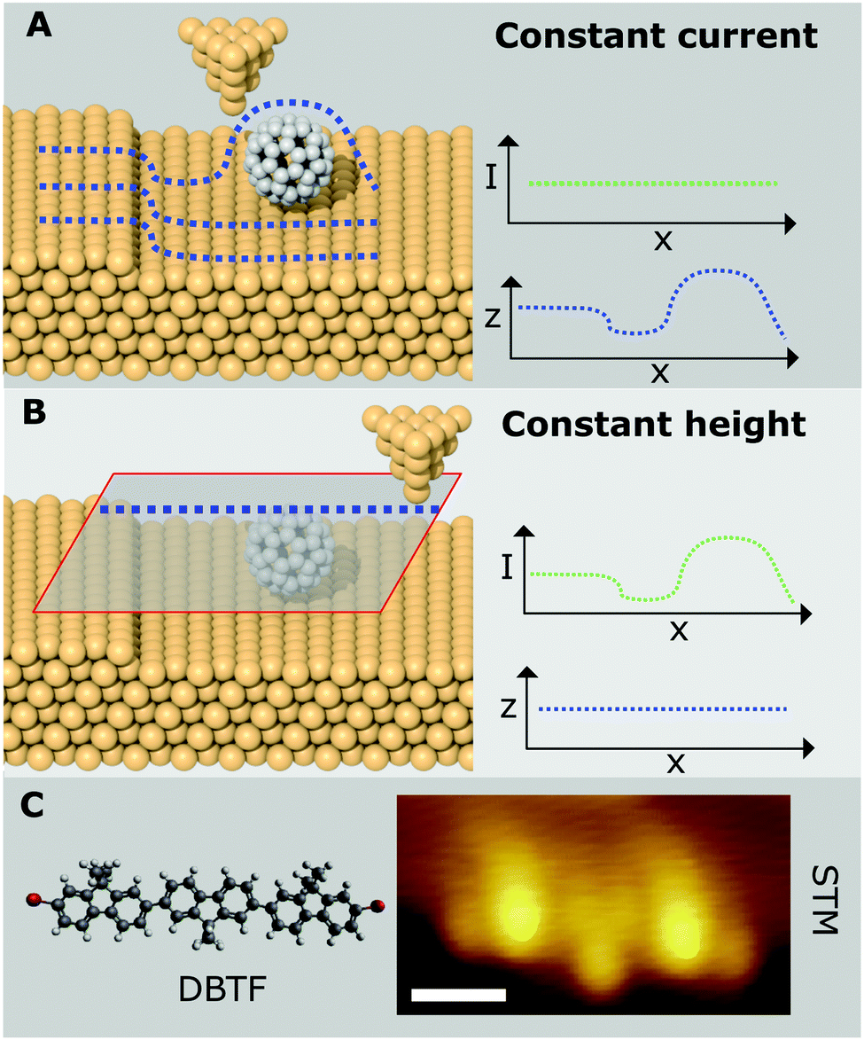Fig. 1 Outline of SPM image acquisition and example of molecular characterisation. (A) Schematic showing image acquisition via a series of line profiles in constant current operation of STM. (B) Operation of STM in constant-height mode. (C) Example of STM characterisation of a single DBTF molecule via STM¹⁰ [scale bar = 1 nm, V_gap = −0.4 V, I_t = 5.5 pA]. STM image in (C) reproduced from ref. 10 with permission from John Wiley & Sons, Inc., Copyright 2012.

An STM image is produced by obtaining a series of line scans (shown in Fig. 1A) which are then combined to form a 2D image. In constant current mode I is maintained at a fixed set-point, typically a few pA, and the resultant image therefore shows the variation in z as the probe is scanned over the surface. In constant height mode images will show the variation in I with tip position. It is important to note that the measured current, for a finite bias voltage, is proportional to the sum of the contributions for the local density of states (LDOS) from which tunnelling is possible;¹i.e. the measured current is related to the electronic structure of the molecule/substrate, and is not necessarily well correlated to the spatial position of the atomic nuclei. In this respect the path of the probe in constant-current mode does not simply provide a topographic height but is better interpreted as a map of the LDOS. This issue manifests in the characterisation of molecules where molecular orbitals are often delocalised over the molecular species under study, therefore preventing the position of individual atoms, within similar chemical environments (e.g. conjugated aromatic carbons), from being resolved. However, in cases where electronic character is localised over specific chemical moities STM images may be compared (at least as an approximation) to the chemical structure of the molecule under study. An example of this is shown in Fig. 1C where the structure of a brominated terfluorene molecule (α,ω-dibromoterfluorene – DBTF) can be compared with a constant-current STM image;¹⁰ features related to peripheral Br atoms and central fluorene groups are visible. Such electronic structures are often compared with density functional theory (DFT) based simulations of STM images which can help identify molecular structure and conformations.¹¹

Consequently, while STM can provide sub-molecular resolution, it suffers, in common with all SPM techniques, with regards to the non-trivial interpretation of the acquired data. Although DFT studies used in conjunction with STM data often offer good agreement and provide a plausible interpretation of the results (in terms of a more complete appreciation of the expected LDOS), an over reliance on DFT can lead to potential pitfalls as calculating the energy and spatial distribution of molecular orbitals for surface adsorbed species can be challenging (specifically when taking into account hybridisation with electronic surface states).

1.4 ncAFM

The basic premise for ncAFM data acquisition is the same as STM, with images formed line by line. In the case of ncAFM the relevant interaction is the force between probe and molecule–substrate system. The focus within this review is on the use of qPlus implementation of ncAFM (see ref. 12, and citations therein, for details of the technique). An excellent description of the underlying principles of qPlus ncAFM is given in ref. 13, but to summarise: The probe, which is affixed to a tine of a quartz tuning fork, is oscillated at it's resonant frequency, and the interaction between tip and sample results in a change in this resonant frequency. This shift in the resonant frequency, Δf, is the signal measured within ncAFM (in the same way I is recorded in STM) and feedback circuits are used to excite the cantilever at its resonance frequency and keep the oscillation amplitude constant. Similar to STM constant current measurements, the z-height can be adjusted during scanning to keep Δf constant (constant Δf imaging), but within this review we discuss constant height measurements where the z-height of the probe relative to the surface is kept fixed and the Δf signal is recorded as a function of probe position. Practically, all sub-molecular studies are performed within constant height operation due to the non-monotonic response of Δf with respect to z and the requirement that imaging is performed in the repulsive regime.²

The terminology ncAFM is used here, as opposed to dynamic force microscopy (DFM) or frequency modulated AFM (FM-AFM); FM-AFM refers to the fact that the frequency shift, Δf, is the main observable. These terms are occasionally used interchangeably with ncAFM, and for the experiments discussed here the ‘noncontact’ aspect refers to the fact that the method is distinct from the classic ‘contact’ mode of cantilever AFM.

ncAFM and STM techniques are often used in conjunction to characterise molecule–substrate systems and provide complimentary information. ncAFM provides greater lateral resolution, due in part to the shorter interaction range (Pauli-repulsion), and in principle offers a route towards chemical specificity. The image acquisition time for ncAFM is, however, significantly slowly than STM, and so it is common practice to first characterise the molecule–substrate system using STM. In addition, ncAFM images are predominantly acquired in constant height operation which is not always compatible with non-planar molecules. The remainder of the review will focus on the application of the ncAFM technique and interpretation of data acquired for various molecule–substrate systems.

2 Practical steps in accomplishing sub-molecular imaging

While the fundamental physical principles of ultra-high resolution ncAFM imaging of single molecules can be understood on a qualitative level with reference to empirical models (see Section 3.1), the technical steps required to achieve it in practice are somewhat demanding. Fortunately many of these core challenges may now be routinely surmounted using commercially available systems, and so in this section we only highlight those challenges specific to ultra-high resolution imaging of organic molecules with functionalised tips.

It should be noted that sub-molecular resolution can be accomplished with a wide variety of sensors, including conventional silicon cantilevers.¹⁴ We also note that similar contrast can be accomplished even in pure STM via use of similarly functionalised tips and operating at specific tunnelling conditions, however it is generally thought that this contrast arises from a direct ‘transducing’ of the tip–sample force into the tunnel current signal¹⁵ and so broadly the same steps and discussion apply as discussed below. However, practically most of the literature on the topic has used the qPlus sensor^2,12 implementation, and therefore in the following we will assume this is the setup under consideration.

2.1 Sample preparation

Although in principle high resolution can be achieved on almost any atomically flat substrate^14,16 in practice most imaging of organic molecules is done using single metal crystals with low index planes (e.g. Cu(111), Ag(111)). These are easily prepared in UHV, and allow for straightforward preparation of the tip in situ (as described in Section 2.3).

2.1.1 Deposition of organic molecules at low temperature. Most small organic molecules have relatively low diffusion barriers on coinage metal surfaces, and readily aggregate into islands¹⁷ if deposited at room temperature. For the investigation of isolated molecules it is therefore recommended that deposition be performed at low temperature. Practically, this is achieved by direct deposition into the scan head. This is typically done using a thermal effusion (Knudsen) cell filled with a thermally purified powder (99% purity or better) of the required molecule, positioned to face one of the shutters of the SPM cryostat.

The cell is bought up to the required deposition temperature, and once a constant rate of deposition is measured, the shutter to the cryostat is opened for a short period of time. In order to prevent diffusion of the molecules on the surface, the substrate temperature should be prevented from exceeding ∼10 K.

2.1.2 CO deposition. Although techniques vary, typically CO molecules (and other gases) are not deposited via direct (line of sight) deposition, but instead the UHV chamber is backfilled with CO gas up to a pressure on the order of 10⁻⁸ mbar,^2,12 by admitting ultra-high purity gas via a UHV leak valve. The shutters of the cryostat are then opened for a short period to admit the gas (as for the deposition of organic molecules). CO deposition is typically performed after deposition of organic molecules, in order to minimise CO diffusion.

This back-filling technique can result in a large quantity of CO gas being absorbed onto the cryostat shields themselves, therefore once CO gas has been dosed into the system, it is essential to keep the cryostat cold until the experiment is complete to prevent sample contamination.

A number of passivating molecules/atoms have been shown to work for high resolution ncAFM of organic molecules (including CO, xenon, chlorine, bromine, iodine¹⁸), but the overwhelming majority of imaging is performed either with CO, or xenon, mostly due to their ready availability, ease of deposition, and large volume of work describing protocols for their manipulation. The exact choice of passivating agent can have a significant influence on the contrast due to its interaction with the short-range electrostatic field of the molecule¹⁹ (see Section 3.1.5).

2.1.3 Decoupling layers. The use of a thin decoupling layer (e.g. 1–3 monolayers (ML) of NaCl or MgO) is a non-essential, but often used step in sub-molecular contrast imaging. The absorption of molecules onto a thin insulating layer is used in STM studies to decouple the electronic structure by preventing hybridisation of molecular orbital's with the surface.¹³

Generally a low coverage (less than half a monolayer) is preferred, such that patches of clean metal remain for tip preparation. Growth of 2 ML thick islands of NaCl can be achieved by deposition onto the metal crystal outside of the scan head, with a sample temperature of around 293 K. Use of a decoupling layer is more common on reactive metals such as copper, compared to less reactive metals such as silver or gold.

2.2 Construction of the qPlus sensor

Whilst the geometry of the qPlus sensor is well described,¹² practically constructing a complete sensor from scratch requires a degree of experimental skill. Both the attachment of the tuning fork to a suitable base, and the attachment of the metal tip to the end of the free tine of the fork must be done carefully such that the resonant frequency and Q factor of the cantilever are not compromised.

2.3 Tip preparation

Although in principle almost any material can be attached to the end of the qPlus sensor, in practice a typical STM tip material such as W, or PtIr, is normally used. qPlus sensors usually have the tip attached to the end of the tine of the tuning fork via UHV compatible epoxy resin, and, because these epoxies usually breakdown at high-temperature, common STM tip treatment techniques such as heating via electron bombardment cannot easily be implemented. Preparation of the tips in situ is essential before attempting high resolution imaging, and is most often accomplished via voltage pulsing, indentations into the surface, or field emission over the surface. Providing the apex of the probe can be coated in a layer of clean surface material, it is usually possible to obtain good resolution even with untreated tips. Nonetheless ex situ preparation techniques such as focused ion beam (to improve the macroscopic radius of curvature),²⁰ or in situ techniques such as field ion microscopy (which can be used to clean the probe apex without heating) are recommended in order to improve reproducibility between experiments. Currently tip preparation is a manual, time consuming process, but recent work offers the exciting possibility this process may be automated via the use of machine learning based image recognition.²¹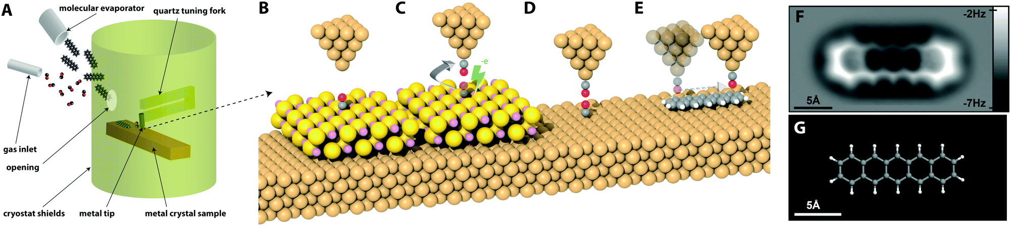

2.3.1 Tip functionalisation. The creation of a functionalised tip itself is an essential part of the imaging process in high resolution ncAFM, and requires some skill in the preparation of clean metal tips via STM methods in situ before it can be attempted. In the discussion below we assume the functionalising molecule to be CO as this is the most commonly used approach (see schematic in Fig. 2A–E).

Fig. 2 Overview of the setup and procedure for generating a suitable surface and tip for the high resolution imaging of absorbed organic molecules. (A) Cartoon showing the setup required for in situ deposition of organic molecules and gas molecules onto a cold metal sample (not to scale), as noted in the text, typically gas and molecular deposition would be done sequentially, and not simultaneously as shown in the schematic. (B) Positioning of metal tip apex over CO molecule absorbed on a 2ML NaCl/Cu(111) island. (C) Excitation of the CO molecule by tunnelling electrons causes the molecule to desorb from the surface and attach itself to the tip. (D) The CO functionalised tip is then characterised on a CO molecule absorbed on the clean Cu(111) surface. (E) An absorbed organic molecule is then imaged in constant height mode using the functionalised tip. (F) constant height Δf image of pentacene molecule absorbed on Cu(111) taken from Gross et al. (G) Ball-and-stick model of pentacene molecule on same scale.² Image (F) from L. Gross, F. Mohn, N. Moll, P. Liljeroth and G. Meyer, Science, 2009, 325, 1110–1114. Reprinted with permission from AAAS, copyright 2009.

First, a clean metal tip should be prepared by controlled crashing of the tip into the metal surface, and good STM resolution should be achieved on both the CO molecule, and the organic molecule to be imaged. It is also desirable that the frequency shift (Δf) of the tip during normal STM operation is relatively small as this indicates a sharp tip apex. The pickup of the desired molecule is then accomplished by positioning the tip over the CO molecule, withdrawing the tip a few hundred pm, and raising the bias above 2.5 V. Transfer of the molecule from the surface the tip is indicated by a jump in the tunnel current.

Although in principle CO can be picked up from the copper surface, in practice this can be hard to achieve due to the high adsorption energy. For this reason, the CO molecule is often picked up from the surface of a NaCl bilayer, as the binding strength to the surface is dramatically reduced.² CO pickup on less reactive surfaces (e.g. Au(111) or Ag(111)) is often easier to achieve, and conversely pickup from more reactive surfaces (e.g. Ir(111)) may be extremely difficult to perform reproducibly.²²

However the transfer is accomplished, it is important to confirm the successful transfer has occurred by characterising the resulting tip apex on other nearby CO molecules. The characteristic contrast change for CO on the Cu(111) substrate is a switch from the imaging of CO molecules as depressions, to a characteristic “sombrero” shape during conventional STM.²

2.4 Practical considerations for imaging

In the standard implementation of qPlus ncAFM, performing large area scans, and preparing the tip, are best performed in STM constant current mode, rather than in ncAFM feedback, due to the generally superior scan speed and stability. Typically a large area is imaged in STM (e.g. 50–100 nm²), and then a small area of interest (e.g. 5–10 nm²) is located and imaged at high resolution using conventional STM, before the tip is functionalised and ncAFM imaging in constant height mode can proceed.

2.4.1 Drift and creep. An essential element in achieving intramolecular resolution is operating in constant height mode, as contrast is obtained only in the repulsive part of the tip–sample interaction, where it is exceptionally difficult to maintain stable imaging using conventional Δf based feedback. Because of the exceptionally strong dependence of the tip–sample force with distance, and long scan times, drift rates on the order of less than 0.5 pm min⁻¹ are required. Practically, this can be accomplished by ensuring that the microscope is at thermal equilibrium before starting imaging. It is also necessary to ensure that no residual piezoelectric creep is present. This is typically done by placing the tip in the required area, and waiting for an extended period. Depending on the exact conditions, and scanner configuration, it may be necessary to wait for upwards of 12 hours before the creep becomes small enough to allow for stable imaging.

2.4.2 Amplitude calibration. The response of the cantilever in ncAFM is recorded as an electrical signal, and an accurate calibration to convert this into a physical oscillation is mandatory. Due to the small oscillation amplitudes typically used during sub-molecular imaging, it is advisable to use a normalised average tunnel current method calibration method similar to that introduced by Sugimoto et al.²³

Because of the variation between different sensors, each sensor must be calibrated separately.

2.4.3 Crosstalk. Most low temperature instruments now permit simultaneous measurement of STM and ncAFM channels. Depending on the exact instrumental set up, it is possible for the tunnel current signal to capacitively couple to, and distort, the cantilever response channel.²⁴ Because it can be difficult to separate crosstalk effects from genuine force interactions, the behaviour of the ncAFM channels in the presence of significant current should be checked on a well-defined metallic substrate before investigating molecular samples. Steps that can reduce crosstalk include: the use of a high bandwidth tunnel current pre-amplifier, biasing the sample and grounding the tip, and using a separate wire for tunnel current collection rather than an integrated electrode. Whilst use of a separate wire for tunnel current collection is in principle preferred, attachment of the wire is in practice often difficult and can easily significantly modify the Q factor and resonant frequency of the sensor.

2.4.4 Force inversion. Whilst not a requirement for standard imaging, it is often desirable to extract quantitative force data from intramolecular resolution studies. If this is desired a method must be selected for the inversion of the frequency shift to vertical tip sample force. Because the frequency shift is, to a first approximation, proportional to −dF/dz, this requires an integration of the complete frequency shift curve from a distance at which an unperturbed oscillation occurs, to the point of interest. Although several integration several schemes exist, the most commonly used is that implemented by the Sader–Jarvis algorithm,²⁵ but it should be noted that recent work suggests there are limits to its applicability depending on the precise nature of the tip sample interaction.²⁶ Additionally, in general, the total tip sample force is not the quantity of interest, as this is dependent on the shape of the (generally uncontrolled) macroscopic tip apex. Instead, usually the quantity of interest is the site-specific (short range) force between the molecule and the last few atoms of the tip apex. In order to extract this quantity the non-site-specific (long-range) forces must be removed. This is best done by acquiring a Δf(z) curve over the same height range away from the molecule (where no contrast is visible), subtracting this from the Δf(z) curve taken on top of the molecule, to produce a “short range” Δf(z) curve, which can then be inverted using the Sader–Jarvis algorithm described above. This protocol assumes a suitable clear area of surface is available close to the molecule, where this is not the case (e.g. in the case of a close packed monolayer of molecules) accurate determination of the site-specific forces may be subject to significant uncertainties.

3 Interpretation of sub-molecular contrast at the single bond level

In this section we focus on the atomic scale physical/chemical forces present in the tip–sample junction, and their role in accurate interpretation of the experimental data.

3.1 Forces in the tip–sample junction

In ncAFM, image contrast arises explicitly from the sum of all of the atomic scale forces that arise in the complete tip–sample junction (including contributions from the metallic tip, the functionalising molecule, the molecule under investigation, and the underlying substrate), and the mechanical response of the atoms in the junction to these forces. Therefore, we will elucidate the key components that result in the production of intramolecular contrast, and describe the state-of-the-art in their interpretation by comparison to different modelling techniques. In the following sections we examine each of these forces in the junction in detail, but it is instructive to first examine a representative image (see Fig. 2F) and cover, qualitatively, the key features. Examining Fig. 2F, we first note that the images are maps of frequency shift (Δf) – i.e. the change in the resonant frequency of the cantilever due to the tip sample force. The relationship between force and frequency is complex (see Section 2.4.4), but to first order we can assume that the frequency shift Δf is proportional to the inverse force gradient −dF/dz. To a very rough approximation we can normally assume that more positive (bright) features correspond to an area of repulsive force, and more negative (darker) areas correspond to more attractive interactions.

3.1.1 Non-site specific interactions – the “background”. Inspecting the image further, the molecule sits within a uniform grey background. This corresponds to regions where the tip is far above the substrate such that the force on the tip is uniform (generally uniformly attractive dispersion and electrostatic forces), i.e. we see only non-site specific (i.e. those providing no atomic scale contrast) forces arising from the bulk interaction between the tip and substrate which provide a background on which all the other interactions sit.

3.1.2 Local dispersion interactions – the “halo”. The net attractive interaction arising from the dispersion interaction between all of the atoms of the molecule, and the atoms at the probe apex, results in an attractive “well” which shows up as a dark (negative frequency shift) feature in constant height imaging, at close approach this results in a dark halo in which the bright geometric structure of the molecule sits.

3.1.3 Pauli repulsion – the “carbon backbone”. The onset of repulsive interactions due to the overlap of the electron orbitals of the tip apex and the molecule is the fundamental origin of intramolecular contrast in tip functionalised ncAFM. As a first order approximation, the magnitude of the repulsive interaction can be considered proportional to the charge density in the space that the tip apex is attempting to probe. Because the total charge density closely mirrors the bonding structure of the molecule, the result is an image which closely mirrors the classic “ball and stick” models used to describe molecular structure (see Fig. 2G). As a repulsive interaction, these features typically show up as bright in constant height imaging (more positive frequency shift) which sit within the dark attractive halo of the dispersion interaction (see above). However, it must be stressed that this is only a first order approximation – as detailed below there are significant differences between maps of the charge density of the molecular system and the ncAFM images, which arise from the subtle interplay of the different forces in the junction, the finite size of the terminating atom, and the response of the probe particle at the probe apex.

3.1.4 Chemical bonding. The key mechanism behind tip functionalised ncAFM is that the addition of a passivating unit to the end of the tip apex inhibits chemical bonding between the tip and molecule, reducing the magnitude of the tip–sample force; preventing the molecule being picked up, or displaced, during close approach of the tip. For this reason forces resulting from chemical bonding between tip and surface are assumed to be negligible in the following discussion.

3.1.5 Local electrostatic interactions. In ncAFM there is often a net long-range electrostatic interaction between the bulk tip apex and the surface, which can be measured and used to determine the difference in workfunction between two materials. However, for the purposes of intramolecular contrast the quantity of interest is the local electrostatic field that arises over the molecule due to localised partial charges. How this local field affects the imaging depends on whether the probe apex itself also has a net charge or dipole, and it is trivial to note that accumulation of charge density (for example due to bonding within the molecule) can also result in a localised electrostatic field, and so effects due to increased charge density and local electrostatics cannot be simply disentangled.

3.2 Response of the probe particle – distortions in imaging

Although it is often easy to make a one-to-one comparison between the image and a structural model of the molecule, some features are somewhat distorted compared to the ball and stick model. In particular some features appear more elongated than a simple structural model would suggest. Key to correctly interpreting these features is an understanding that due to the extremely close approach of the probe apex to the molecule, the probe can no longer be considered to be a “weakly perturbing” interaction (as is often assumed in conventional STM for example). As such we cannot assume that the images produce a simple map of the unperturbed state of the molecule, but instead must explicitly consider the dynamic response of the complete system. Fortunately, an important simplifying assumption that can be made is that the attachment of the probe particle to the metal tip apex is the most mechanically flexible part of the system, and therefore that almost all the relaxation that occurs in the junction will occur at this position. Moreover, it has been shown that a good qualitative understanding of these systems can be extracted from simulations that assume simple empirical potentials between the probe and the surface geometry, assuming that only the probe particle is able to move.¹⁵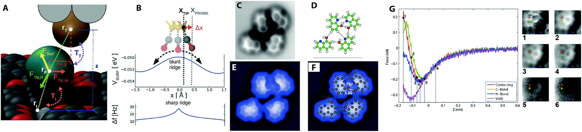

3.2.1 Flexibility of adsorbed CO. Direct evidence of flexibility of adsorbed CO in the context of SPM imaging comes from combined experimental and theoretical studies.⁹ The flexibility of the CO probe was first explicitly described in the context of imaging organic molecules as a “enhancement” effect,⁹ and was supported by detailed DFT calculations showing how the tip apex geometry changed during simulated imaging. On this basis Hapala et al.¹⁵ developed a simple model using empirical potentials to approximate the CO–molecule interaction to rapidly create simulated images (see Fig. 3A).

Fig. 3 Key results in understanding intermolecular bond resolution in ncAFM. (A) Overview of the PPM probe particle and the forces acting upon it on a PTCDA island.¹⁵ (B) Schematic showing the principal of the sharpening of features due to the deflection of the probe particle over a ridge in the potential energy landscape. (C) Constant height Δf image showing contrast in expected hydrogen bonding locations in a small hydroxyquiline (8-hq) molecular island absorbed on the Cu(111) surface.²⁷ (D) Ball and stick model showing proposed geometries and location of expected hydrogen bonds. (E) Simulated image of 8-hq island using the PPM. (F) Same image but with ball and stick model and proposed hydrogen bonding locations overlaid. (G) Experimental 3D force map data showing F(z) curves, and 2D XY force images over an NTCDI Island on Ag:Si(111).²⁸ Images (A–B) reprinted with permission from P. Hapala, G. Kichin, C. Wagner, F. S. Tautz, R. Temirov and P. Jelínek, Phys. Rev. B: Condens. Matter Mater. Phys., 2014, 90, 085421. Copyright (2014) by the American Physical Society. Images (C–F) from J. Zhang, P. Chen, B. Yuan, W. Ji, Z. Cheng and X. Qiu, Science, 2013, 342, 611–614. Reprinted with permission from AAAS, copyright 2013. Image (G) reproduced with permission under a Creative Commons license from ref. 28, Copyright 2014.

Because of the low lateral stiffness of the CO molecule, the particle in the tip–sample junction has the tendency to deflect sideways when approaching a ridge in the potential energy landscape (see Fig. 3B). As a result any ridge experienced by the probe particle will have the tendency to sharpen into a line connecting two centres. Importantly, as demonstrated in simulations using the probe particle model (where interactions can only arise from simple steric hindrance mediated by the Lennard Jones potential) similar ridges will arise even if there is no charge density in the space between two atoms (see Fig. 3E and F).

Consequently, the critical question becomes to what extent the probe particle is able to penetrate the space between two atoms, and to understand the physical phenomena at work (cf. the related concept of solvent excluded volume when considering the penetration of water into protein structures). The case of hydrogen bonding between surface absorbed molecules has been particularly controversial, with initial reports directly assigning ridges in the position of expected hydrogen bonds to direct observation of the bonding itself (see Fig. 3C and D).²⁷

Simulations using the probe particle model (see Fig. 3E and F), and subsequent experimental results from molecular junctions where no hydrogen bonding is expected to occur^15,31 reproduced similar contrast, despite not taking into account any hydrogen bonding effects, and other results confirmed that the hydrogen bonding contrast only arises in the repulsive regime where deflection and steric effects are key²⁸ (see Fig. 3G). Atoms in close proximity to each other will appear to be linked even if no bonding between them is present due to simple steric hindrance effects resulting from the finite radius of curvature of the involved atoms. Steric hindrance arguments also suggest that much of the charge density in the intervening space due to any bonding is in fact already inaccessible to the probe due to the finite radius of the probe atom itself. In the case of hydrogen bonding, there remains no good theoretical justification for how hydrogen bonding can, even in principle, contribute to the contrast using accepted models for how intramolecular contrast arises. It is important to note that even with a rigid probe, steric hindrance effects will still result in a ridge between two atoms in close proximity,³² and therefore the deflection normally only serves to enhance an already existing effect.

Covalent bonding presents an interesting case, as the same probe particle model also reproduces the contrast in the positions of expected covalent bonds, also without taking into account the accumulated charge density in the bond, and thus a question arises as to what extent the charge density between the atoms contributes to the overall contrast. Some confidence that the charge density associated with covalent bonding does affect the imaging can be taken from pronounced node-like features in the imaging of triple bonds,³³ which cannot be reproduced in models using simple Lennard Jones potentials.

3.2.2 Electrostatics. An additional subtlety arises from the short-range electrostatic force field above molecules with significant localised charges, and their interaction with the probe particle, which may have itself localised charges. The imaging of TOAT molecules absorbed on metal surfaces with CO and xenon functionalised tips was have shown to display significant, tip dependent, distortions in the structure of the molecule at close approach (see Fig. 4A and B), modelling of which necessitates consideration of the different local charges of the probe particle.³⁴ It is therefore clear that the deflection of the probe particle in the junction can be strongly affected by a number of factors, which can only be elucidated via a combination of first principles modelling and empirical potentials to allow for high resolution simulations of the complete system, which are extremely difficult to achieve using ab initio simulation techniques alone.

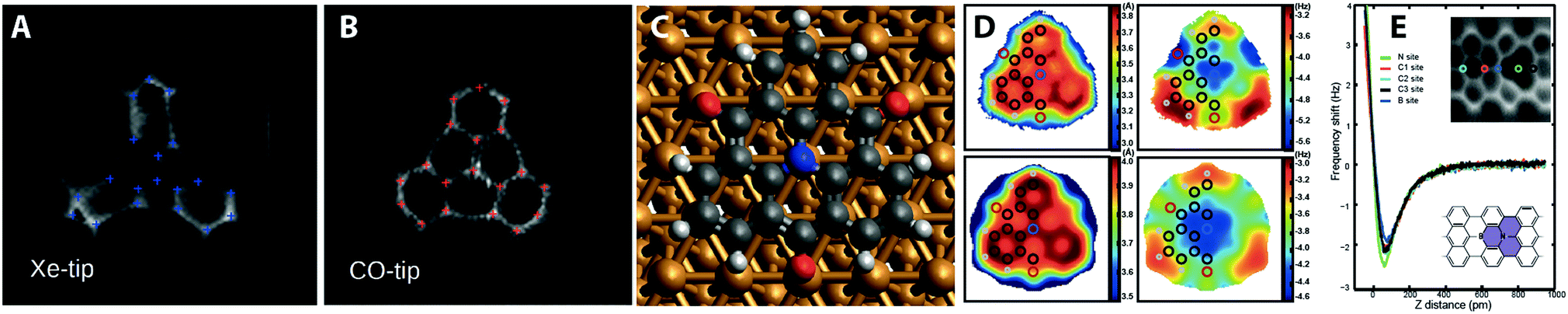Fig. 4 Examples mapping the local electrostatic field, and chemical identity of atoms in small molecules. (A) TOAT molecule imaged with a xenon tip and a (B) CO tip showing distortion due to the local electrostatic field of the molecule.¹⁹ (C) Ball and stick model showing TOAT molecule adsorbed on Cu(111) surface.²⁹ (D) experimental (top) and calculated (bottom) Z* and Δf* maps of TOAT molecule highlighting local variation over chemically distinct atoms.²⁹ (E) Identification of substitutional boron and nitrogen atoms in a surface synthesised graphene nanoribbon.³⁰ Images (A) and (B) reproduced with permission under a Creative Commons license from ref. 19, copyright 2016. Images (C) and (D) reprinted with permission from N. J. van der Heijden, P. Hapala, J. A. Rombouts, J. van der Lit, D. Smith, P. Mutombo, M. Švec, P. Jelinek and I. Swart, ACS Nano, 2016, 10, 8517. Copyright 2016 American Chemical Society. Image (E) reproduced with permission under a Creative Commons license from ref. 30, copyright 2018.

3.2.3 Chemical sensitivity. Prior to the development of intramolecular resolution imaging, it had been shown that ncAFM was, in principle, capable of achieving chemical sensitivity during atomic resolution imaging, by comparing the ratio of interactions between different atoms in mixed phase semiconductor blends.³⁵ An open question, therefore, is whether this same sensitivity may be achieved during intramolecular imaging by similar methods, i.e. can the chemical identity of the atoms in a molecule be determined from a high-resolution image using CO terminated tips? Recent work has shown promise in this direction,^20,30 but has highlighted that severe complications arise as the most important interactions in chemical identification (i.e. the chemical interactions), are intrinsically suppressed by the use of a passivating unit on the tip apex. Only by direct comparison to high-quality simulations can attempts at this level of identification be made, and interpretation of the data is not straightforward, as any force difference arising from the difference in the chemical identity of the atom itself is strongly convoluted with geometric effects, and local charges, related to the structure of the molecule (see Fig. 4D and E).

4 Characterising on-surface reactions with ncAFM

From the discussion outlined above it is apparent that individual molecules can be characterised using CO functionalised probes. However ncAFM can also be used to look at the initial, intermediate, and final structures of a reaction. All of the reactions discussed here are performed ‘on-surface’ and as such are confined to a supporting substrate. This on-surface synthesis approach has been seen to give rise to different reaction pathways to that observed in solution based-synthesis and potentially provides new options for influencing and controlling reactions.⁶

4.1 Practical considerations for characterising on-surface reactions

The acquisition time for SPM techniques is slow compared to the timescale of the reactions under study: on-surface diffusion steps will be many orders of magnitude faster than the several minutes typically required to form a ncAFM image. Therefore, in order to allow characterisation of on-surface reactions, studies are usually performed in discrete stages where: (1) reactant molecules are deposited onto a substrate held at a low temperature, allowing the initial precursors to be characterised. (2) Thermal energy is supplied to initiate an aspect of the reaction, i.e. formation of an intermediate/transition state, with the substrate then cooled to allow high resolution image acquisition. (3) Heating the substrate to a higher temperature then allows reaction to progress to completion with high resolution images subsequently acquired at low temperature. In principle it is possible to gain information about the chemical composition of the molecular species under study from ncAFM characterisation (in a similar way to that demonstrated for distinguishing between mixtures of atomic species³⁵). However, as discussed in Section 3.2.3, interpretation of chemical contrast is non-trivial, even when comparison with a known reference material is possible. More accessible, and of considerable importance, is the determination of the bond order of bonds between carbon atoms. Visually a variation in contrast (Δf) has been observed between single and triple carbon–carbon bonds which has been attributed to a variation in charge density (which in turn gives rise to a variation in Pauli repulsion between probe and molecule and is displayed as change in the measured Δf signal).⁹ Nonetheless, the measurement of bond length and bond order via CO functionalised ncAFM has important limitations – the deflection of the CO provides an enhancement effect which allows these small variations to be observed, but the same effect means that direct measurement of the true bond lengths is not possible, as the degree of distortion can be modified by local electrostatic fields¹⁹ and variations in vdW background,³⁹ and is also dependent on the lateral stiffness of the adsorbed CO. Therefore direct measurement of the bond lengths is usually only possible in parallel with high quality simulation, or by complex ‘de-skewing’ procedures⁴⁰

It is also possible to estimate the adsorption height of the molecular species above the surface, but this requires calibration to a reference point⁴¹ (such as X-ray standing wave based analysis). In the absence of absolute height reference data ncAFM can still be used to determine the relative adsorption heights across an adsorbed molecule.

4.2 Synthesis and characterisation of graphene based nanostructures

Graphene based structures, including graphene nanoribbons (GNRs), have received much attention due to their electrical and optical adsorption properties as well as the potential for their applications within device structures (e.g. as molecular wires⁴²). However, the atomically precise formation of GNRs is challenging, as is the characterisation of the resultant structures. Defects, in particular atomic scale defects, can have important effects upon the desired characteristics of any device based upon GNRs. Therefore SPM techniques provide a method which allows the reaction steps to be identified as well as facilitating structural characterisation of the resultant product.

The first on-surface synthesis of GNRs was shown by Cai et al.⁴³ and was based upon the use of dibromo functionalised bianthracene units (1) which were observed to couple together on a Au(111) surface to form linear chains (see Fig. 5A for mechanism). This type of covalent coupling reaction, based on Ullmann coupling (iodine functionalised aryls coupled over a copper catalyst), was first applied to the formation of covalently coupled molecular architectures by Grill et al.⁴⁴ The reaction mechanism for the formation of GNRs was postulated to be a two-step process involving; (i) C–C coupling giving rise to a non-planar product and (ii) a cyclodehydrogenation reaction forming the aromatic structure of the GNR. This assignment was based upon distinct structural differences at different stages of the reaction, as shown within STM images (an STM image showing a GNR following the cyclodehydrogenation step on Au(111) is shown in Fig. 5B). However the STM data (while supporting the proposed mechanism) does not show the sub-molecular resolution offered by ncAFM to allow the spatial position of the bonds to be observed.

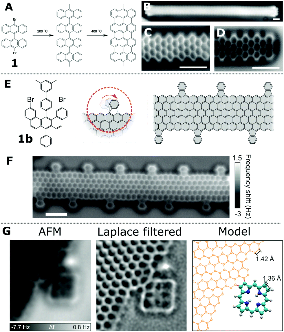Fig. 5 ncAFM characterisation of 2D graphene structures. (A) Schematic showing the two-step formation of graphene nanoribbons (GNRs) using a dibromo bianthracene precursor (1). (B) STM [scale bar 1 nm] and (C and D) ncAFM images of GNRs with armchair edge structure visible in ncAFM images³⁶ [scale bars 1 nm]. (E) Scheme for the synthesis of functional GNRs via an alternative precursor (1b); proposed structure and ncAFM images, shown in (F), [scale bar 1 nm].³⁷ (G) Characterisation of pyrrole units fused to a graphene sheet imaged via ncAFM.³⁸ Images (B and D) reproduced with permission under a Creative Commons license from ref. 36, copyright 2013. Images (E and F) reprinted by permission from P. Ruffieux, S. Wang, B. Yang, C. Sánchez-Sánchez, J. Liu, T. Dienel, L. Talirz, P. Shinde, C. A. Pignedoli, D. Passerone, T. Dumslaff, X. Feng, K. Müllen and R. Fasel, Nature, 2016, 531, 489, Copyright 2016. Image (G) reprinted by permission from Y. He, M. Garnica, F. Bischoff, J. Ducke, M.-L. Bocquet, M. Batzill, W. Auwärter and J. V. Barth, Nat. Chem., 2017, 9, 33–38, copyright 2017.

ncAFM studies of the resultant GNRs allow characterisation of the edge structure of GNRs (either armchair⁴⁵ or a zig-zag³⁷ motif). A simple visual inspection of ncAFM images acquired above a GNR shows regions of brighter contrast (positive values of Δf) assigned to the carbon back-bone of the system (Fig. 5C); alternating columns of 3 and 2 fused benzene rings are visible. Such images allow ready characterisation of the edge structure – in the example here the so called ‘armchair’ edge structure is present. Similarly in Fig. 5D the end of a GNR can be observed with the right-hand side being terminated by a ‘zig-zag’ structure. The exact termination of the edge-structure of the GNR (e.g. ‘zig-zag’ or ‘armchair’) has been observed to have an effect on the electronic states⁴² in terms of the energy and delocalisation.

In order to form GNRs with specific edge structures different precursor molecules are required (see Fig. 5A and E for details of two alternative precursor – ref. 45 and 37). Fig. 5E shows the precursor molecule (1b) employed by Ruffieux et al. to produce GNRs with functionalised zig-zag edges.³⁷ The reaction is assumed to progress by a mechanism where the reactant molecules couple via an Ullmann-type reaction and subsequent cyclodehydrogenation. At the activation temperatures required to form the GNRs (573 K)³⁷ the external phenyl groups undergo a ring-closing reaction with the body of the GNR forming a fluoranthene-type sub-unit incorporating a 5-membered ring. This structure, (clearly imaged in the ncAFM images Fig. 5F) allows structural characterisation of the resultant GNR and clearly demonstrates that the additional phenyl group fuses to the edge with a cyclic motif and is not connected via a σ bond as in the precursor molecule (1b).

Additional functionalisation of graphene structures has been demonstrated by fusing tetrapyrroles (free-base porphyrins, 2H-P) to the edges of extended graphene structures.³⁸ In the work by He et al. a Ag(111) surface, partially covered with graphene structures, was exposed to 2H-P (with 2H-P found to adsorb as individual molecules on bare Ag(111) as well as at the edges of the graphene structures). A coupling reaction was initiated by annealing the sample at 620 K, with the resulting ncAFM characterisation indicating the precise nature of the bonding between 2H-P and the graphene structures (shown in Fig. 5G). The bond resolving power of ncAFM can also facilitate the investigation and characterisation of local ‘defects’ within graphene structures. In the work by Liu et al.⁴⁶ 4 and 8 membered rings can be observed within the graphene structure. Such defects are important as they may be beneficial with regards to tuning the electronic properties of the structures.

4.3 Studying the evolution of on-surface reaction

Cyclisation processes are a feature in many reaction pathways, with the conversion of neighbouring alkyne units to aromatic rings being common place. Work by Oteyza et al.³³ shows how the reactants and products of a cyclisation reaction involving enediynes can be studied using ncAFM. Such cyclisation reactions can result in the formation of a variety of products, and therefore detailed characterisation via ensemble techniques can be non-trivial. ncAFM therefore offers a route towards single-molecule characterisation of the reaction pathway. The reactant molecule 2-bis((2-ethynylphenyl)ethynyl)benzene (2, see Fig. 6A) was deposited on a Ag(100) surface held at room temperature and subsequently imaged at ≤7 K. Initial characterisation of the reactants and products was carried out using STM (with the sample annealed to T > 360 K to initiate the reaction). High-resolution ncAFM images allow the reactant molecular features to be assigned to the aromatic rings and alkyne groups (see Fig. 6A). Variation in contrast at the position of the triple bond can be observed for 2 within the ncAFM image as an enhanced value of Δf (similar contrast is not visible within the STM image).

Fig. 6 Details of on-surface cyclisation reactions where products and reactants are characterised by ncAFM. (A) Chemical structure of reactant molecule, 1,2-bis((2-ethynylphenyl)ethynyl)benzene (2), as well as STM and ncAFM image of molecule on the Ag(100) substrate [scale bars 0.3 nm]. (B–D) Chemical structures and ncAFM images of the on-surface reaction products of 2 on Ag(100) following heating to >360 K [scale bars 0.3 nm]. (E) Reactant and product species for the cross-coupling and cyclisation of 1,2-bis(2-ethynylphenyl)ethyne on Ag(100). (F) Graph showing the systematic heating of Ag(100) surface with adsorbed 6 to a range of temperatures between 290 and 460 K. (G) Details of the relative abundance of the experimentally observed species (7 being the product, with i and ii being intermediates) during a series of annealing steps (temperature profile shown in (F)) [(A–D) from ref. 33 (E–G) from ref. 47]. Images (A–D) from D. G. de Oteyza, P. Gorman, Y.-C. Chen, S. Wickenburg, A. Riss, D. J. Mowbray, G. Etkin, Z. Pedramrazi, H.-Z. Tsai, A. Rubio, M. F. Crommie and F. R. Fischer, Science, 2013, 340, 1434–1437. Reprinted with permission from AAAS, copyright 2013. Images (E–G) reprinted by permission from A. Riss, A. P. Paz, S. Wickenburg, H.-Z. Tsai, D. G. De Oteyza, A. J. Bradley, M. M. Ugeda, P. Gorman, H. S. Jung, M. F. Crommie, A. Rubio and F. R. Fischer, Nat. Chem., 2016, 8, 678–683, copyright 2016.

Following heating of the surface (T > 90 °C) 3 reactant products (3, 4, 5), all displaying distinct and different appearances within STM images, were identified (in the ratio 3 : 4 : 5 = (51 ± 7%) : (28 ± 5%) : (7 ± 3%)). From ncAFM characterisation of the product structures the newly formed six-, five-, and four-membered rings can be seen within the product molecules (see Fig. 6B–D) and allows the structures of these species to be inferred. From this knowledge of the structure of the reactants and products Oteyza et al. were able to propose the thermal reaction pathways, supported by DFT based calculations.³³

A similar reaction system detailing cyclisation was the subject of a study by Riss et al.⁴⁷ where step-wise bimolecular enediyne coupling was observed on a Ag(100) surface. Here the temporal evolution of the reaction was observed (focusing on the conversion of intermediate structures to products as a function of reaction temperature). In order to identify the transient intermediates present within a multi-step reaction, thermal cycling and quenching of the system was employed. The molecule, 1,2-bis(2-ethynyl phenyl)ethyne 6 (Fig. 6E), was deposited on to Ag(100) substrate and characterised at ∼4 K using ncAFM. This approach enabled identification of the rings and triple bond within the structure (similar to that seen in Fig. 6A) of the reactant molecule (with both cis and trans forms being observed).

To track the progress of the reaction as a function of temperature the sample was systematically heated to a range of temperatures between 290 and 460 K. In each case the sample was heated then allowed to cool to room temperature (∼1 hour for each cycle – see Fig. 6F) with the sample then cooled to ∼4 K for characterisation of the products.

The dimerisation of 6 was studied and it was noted that, following initial coupling, the dimer progressed through various degrees of cyclisation. The fully cyclised dimer product is shown in Fig. 6E (7) and the relative abundance of the uncyclised (i), half-cyclised (ii), and fully cyclised (7) dimers were characterised for each temperature cycle (Fig. 6G). The relative ratio of the abundance of the respective species gradually shifts towards molecules with a higher degree of cyclisation following each anneal step. This suggests that the partially cyclised molecules are transient intermediates on the way to the fully cyclised dimer species. The total number of molecules was not observed to significantly decrease over the reaction; suggesting that desorption or trapping of intermediate species at surface sites (e.g. step-edges or defects) does not play an important role. In concert with DFT calculations it is possible to obtain details of the reaction mechanism (by incorporating details of the structure of the known transition states).

It is also possible to obtain information about the bond order (which on a simplistic level can be related to the bond number, i.e. a triple C–C has a bond number of 3, while C–H has 1). This information can be invaluable in determining the structure of a molecular species via ncAFM characterisation. Schuler et al. showed that it is possible to reversibly induce the Bergman cyclisation of a diyne with a ten-membered ring using the probe to perform atomic manipulation between the two structures (see Fig. 7A);⁴⁸ resulting in an increase/decrease in bond order within the intramolecular carbon–carbon bonds within the molecule.

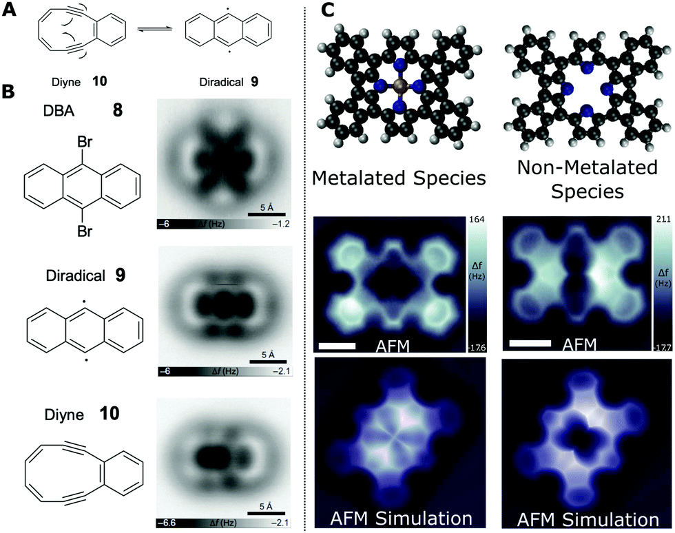Fig. 7 Examples of characterisation of bond order and chemical structure for carbon containing species. (A) Scheme showing the reversible Bergman cyclisation of the cyclic diyne 3,4-benzocyclodeca-3,7,9-triene-1,5-diyne (4) to generate the 9,10-didehydroanthracene diradical (5). (B) Structures and AFM imaging of the starting material, reaction intermediates and product formed by successive STM debromination and subsequent cyclisation. ncAFM images of the molecules were acquired on NaCl(2ML)/Cu(111) using a CO tip ((A and B) from ref. 48). (C) Chemical structure, ncAFM images and simulated ncAFM images of metalated and non-metalated planarised porphyrin monomers on Au(111) ((C) from ref. 50) [scale bars 0.5 nm]. Images (A and B) reprinted by permission from B. Schuler, S. Fatayer, F. Mohn, N. Moll, N. Pavlicek, G. Meyer, D. Peña and L. Gross, Nat. Chem., 2016, 8, 220–224, copyright 2016. Image (C) reproduced from B. Cirera, B. Torre, D. Moreno, M. Ondrácek, R. Zboril, R. Miranda, P. Jelínek and D. Écija, Chem. Mater., 2019, 31, 3248–3256. Copyright 2019 American Chemical Society.

A bromine functionalised anthracene molecule (9,10-dibromoanthracene – DBA, 8) was deposited onto a bilayer NaCl film on Cu(111). Following characteristaion by ncAFM (see Fig. 7B) the probe was positioned above the bright (positive Δf) features corresponding to the position of the Br substituents. Both Br atoms were removed via injection of electrons (achieved by increasing the bias applied to the sample for a short time – a so called ‘bias pulse’, a technique first used to induce local on-surface chemical bond-breaking by Hla et al.⁴⁹). The first Br is removed using a bias pulse at 1.6 V and the second Br can be removed using a higher voltage pulse (3.3 V – 10 seconds of pA current) with the probe withdrawn from the molecule so as to limit the current flow (a high current and elevated bias may induce additional unwanted bond cleavage). This doubly debrominated diradical species was then imaged (see Fig. 7B – diradical 9). It should be noted that the radical species is stabilised by the NaCl film (formation of the species was observed on Cu(111) but conversion to the diyne was not initiated; indicating a strong interaction between the diradical and the Cu surface).

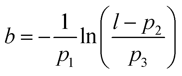
Applying additional bias pulses (1.7 V) above the diradical species results in conversion to a cyclised structure (Fig. 7B – diyne 10). ncAFM images of the resulting product reveal that the structure consists of fused six- and ten-membered rings – suggesting the formation of diyne 4 by homolytic cleavage of the C–C bond shared by two fused benzene rings. Visual analysis reveals the presence of triple bonds (observed to appear with a distinctive elongation perpendicular to the bond direction, as previously found for alkynes imaged by CO tips³³). Detailed analysis provides further information about the bond order of the structure. The values for the Pauling bond order, b, for systems with a carbon-backbone can be calculated using:

where p₁ = 0.6852, p₂ = 1.0979, p₃ = 0.4397 (obtained from fitting the lengths of the carbon–carbon bond within ethane, ethylene, and acetylene⁴⁸). Therefore by measuring the length (l) of the bonds obtained from the ncAFM images and comparing them to the simulated ncAFM images based on DFT calculated structures (thereby taking the flexibility of the CO functionalised tip into account) it is possible to assign the experimentally observed features to structural models. It is important to note that the apparent length of the bonds from the experimentally acquired images have to be compared to a simulated model of apparent distances, not the actual bond lengths as calculated by DFT. This is due to the fact that the tip flexibility results in a distortion of the apparent inter-atomic distances when the probe–sample distance is small (see Section 3.2.1).⁹ This means that although the approach provides some information on variation in bond order within a molecule a direct measurement is not possible.

An example of the utility of comparing simulated ncAFM images (based on the flexible probe model – Section 3.2.1) and experimental data is illustrated in the work by Cirera et al.⁵⁰ A fluorinated free-base porphyrin (5,10,15,20-tetrakis-(4-fluorophenyl)porphyrin, 2H-4FTPP) was studied on a Au(111) surface and observed to undergo a variety of thermally induced chemical transformations (characterised by ncAFM). The 2H-4FTPP species was observed to undergo a ring-closure reaction when heated; annealing at 500 K resulted in the formation of a planar species, with self-metalation (incorporation of Au adatoms into the core of the macrocycle) occurring at 575 K. Structures of the non-metallated and metallated planarised porphyrin species are shown in Fig. 7C.

The structure of the reaction products was determined by comparison with simulated ncAFM images based upon the probe particle model (PPM – see Section 3.2). Fig. 7C shows the ncAFM data for two of the observed planarised species (metalated and non-metalated) alongside simulated ncAFM images based upon molecular models (structures obtained from DFT calculations). While there is qualitative agreement between the simulated and experimentally obtained data, both showing a clear distinction between the metalated and non-metalated species, and a good description of the backbone of the molecule and the expected symmetry of the core, there are nonetheless significant differences in the observed contrast particularly around the metal core, highlighting the need for further progress towards a complete understanding of the contrast formation mechanism for more complex interactions.

5 Conclusions

This review has demonstrated the effectiveness of using scanning probe microscopy, and particularly ncAFM, as a tool for imaging and characterisation of on-surface chemical reactions. It is apparent from the systems discussed that ncAFM provides remarkable images of systems with intramolecular resolution but, importantly, these experiments also provide detailed chemical information for the systems studied. The level of detail is significant, allowing discrimination of individual atoms and/or chemical bonds. Such levels of information are highly unusual in chemistry and although other techniques may provide similar information (e.g. single crystal X-ray diffraction) ncAFM is unparalleled in operating at the single molecule level.

However, we have also sought to demonstrate the experimental challenges and limitations of performing such measurements. Indeed, it should always be recognised that ncAFM, and other SPM measurements, probe molecules adsorbed on a substrate and that the interaction between the molecule of interest and the substrate influences the properties observed. We have also discussed the importance of using UHV, low temperature conditions to perform ncAFM imaging and the factors associated with the choice of tip and probe molecule. We emphasise the importance of detailed studies that seek to confirm the exact nature of features observed in ncAFM images and how misassignment of features is a significant problem in the field.

It is apparent that scanning probe microscopy, and in particular ncAFM, is a remarkable advance which allow the identification of individual molecules and even reaction processes. These approaches will continue to grow in importance in the development of our understanding of single molecule processes and we fully anticipate that ncAFM will become a tool used across the chemical sciences.

Conflicts of interest

There are no conflicts to declare.

Acknowledgements

Alex Saywell acknowledges support via a Royal Society University Research Fellowship. NRC acknowledges financial support from the UK Engineering and Physical Sciences Research Council (EP/S002995/1). Adam Sweetman acknowledges support via a Royal Society University Research Fellowship and via the ERC Grant 3DMOSHBOND. The authors also acknowledge Shashank S. Harivyasi for his assistance in assembling the figures in this paper.

References

1. R. Wiesendanger, Scanning Probe Microscopy and Spectroscopy: Methods and Applications, Cambridge University Press, Cambridge England, New York, 2010.
2. L. Gross, F. Mohn, N. Moll, P. Liljeroth and G. Meyer, Science, 2009, 325, 1110–1114.
3. K. Ø. Hanssen, B. Schuler, A. J. Williams, T. B. Demissie, E. Hansen, J. H. Andersen, J. Svenson, K. Blinov, M. Repisky, F. Mohn, G. Meyer, J.-S. Svendsen, K. Ruud, M. Elyashberg, L. Gross, M. Jaspars and J. Isaksson, Angew. Chem., Int. Ed., 2012, 51, 12238–12241.
4. B. Schuler, G. Meyer, D. Peña, O. C. Mullins and L. Gross, J. Am. Chem. Soc., 2015, 137, 9870–9876.
5. Q. Fan, J. M. Gottfried and J. Zhu, Acc. Chem. Res., 2015, 48, 2484–2494.
6. S. Clair and D. G. Oteyza, Chem. Rev., 2019, 119, 4717–4776.
7. L. Grill, J. Phys.: Condens. Matter, 2010, 22, 84023.
8. R. Lindner and A. Kühnle, ChemPhysChem, 2015, 16, 1582–1592.
9. L. Gross, F. Mohn, N. Moll, B. Schuler, A. Criado, E. Guitian, D. Pena, A. Gourdon and G. Meyer, Science, 2012, 337, 1326–1329.
10. A. Saywell, J. Schwarz, S. Hecht and L. Grill, Angew. Chem., Int. Ed., 2012, 51, 5096–5100.
11. A. Saywell, W. Greń, G. Franc, A. Gourdon, X. Bouju and L. Grill, J. Phys. Chem. C, 2014, 118, 1719–1728.
12. F. J. Giessibl, Rev. Sci. Instrum., 2019, 90, 11101.
13. L. Gross, B. Schuler, N. Pavliček, S. Fatayer, Z. Majzik, N. Moll, D. Peña and G. Meyer, Angew. Chem., Int. Ed., 2018, 57, 3888–3908.
14. C. Moreno, O. Stetsovych, T. K. Shimizu and O. Custance, Nano Lett., 2015, 15, 2257–2262.
15. P. Hapala, G. Kichin, C. Wagner, F. S. Tautz, R. Temirov and P. Jelínek, Phys. Rev. B: Condens. Matter Mater. Phys., 2014, 90, 085421.
16. A. Sweetman, S. Jarvis, P. Rahe, N. Champness, L. Kantorovich and P. Moriarty, Phys. Rev. B: Condens. Matter Mater. Phys., 2014, 90, 165425.
17. J. V. Barth, Annu. Rev. Phys. Chem., 2007, 58, 375–407.
18. F. Mohn, B. Schuler, L. Gross and G. Meyer, Appl. Phys. Lett., 2013, 102, 73104–73109.
19. P. Hapala, M. Svec, O. Stetsovych, M. Ondracek, P. Mutombo, P. Jelinek, J. van der Lit, N. J. van der Heijden and I. Swart, Nat. Commun., 2016, 7, 11560.
20. S. Kawai, A. S. Foster, T. Björkman, S. Nowakowska, J. Björk, F. F. Canova, L. H. Gade, T. A. Jung and E. Meyer, Nat. Commun., 2016, 7, 11559.
21. O. Gordon, P. D'Hondt, L. Knijff, S. E. Freeney, F. Junqueira, P. Moriarty and I. Swart, Rev. Sci. Instrum., 2019, 90, 103704.
22. M. P. Boneschanscher, J. Van Der Lit, Z. Sun, I. Swart, P. Liljeroth and D. Vanmaekelbergh, ACS Nano, 2012, 6, 10216–10221.
23. Y. Sugimoto and J. Onoda, Appl. Phys. Lett., 2019, 115, 173104.
24. Z. Majzik, M. Setvín, A. Bettac, A. Feltz, V. Cháb and P. Jelínek, Beilstein J. Nanotechnol., 2012, 3, 249–259.
25. J. E. Sader and S. P. Jarvis, Appl. Phys. Lett., 2004, 84, 1801.
26. J. E. Sader, B. D. Hughes, F. Huber and F. J. Giessibl, Nat. Nanotechnol., 2018, 13, 1088–1091.
27. J. Zhang, P. Chen, B. Yuan, W. Ji, Z. Cheng and X. Qiu, Science, 2013, 342, 611–614.
28. A. M. Sweetman, S. P. Jarvis, H. Sang, I. Lekkas, P. Rahe, Y. Wang, J. Wang, N. R. Champness, L. Kantorovich and P. Moriarty, Nat. Commun., 2014, 5, 3931.
29. N. J. van der Heijden, P. Hapala, J. A. Rombouts, J. van der Lit, D. Smith, P. Mutombo, M. Švec, P. Jelinek and I. Swart, ACS Nano, 2016, 10, 8517.
30. S. Kawai, S. Nakatsuka, T. Hatakeyama, R. Pawlak, T. Meier, J. Tracey, E. Meyer and A. S. Foster, Sci. Adv., 2018, 4, eaar7181.
31. S. K. Haemaelaeinen, N. V. D. Heijden, J. V. D. Lit, S. D. Hartog, P. Liljeroth and I. Swart, Phys. Rev. Lett., 2014, 113, 186102.
32. H. Mönig, S. Amirjalayer, A. Timmer, Z. Hu, L. Liu, O. Damp, A. Arado, M. Cnudde, C. Alejandro Strassert, W. Ji, M. Rohlfing and H. Fuchs, Nat. Nanotechnol., 2018, 13, 371–375.
33. D. G. de Oteyza, P. Gorman, Y.-C. Chen, S. Wickenburg, A. Riss, D. J. Mowbray, G. Etkin, Z. Pedramrazi, H.-Z. Tsai, A. Rubio, M. F. Crommie and F. R. Fischer, Science, 2013, 340, 1434–1437.
34. M. Ellner, N. Pavliček, P. Pou, B. Schuler, N. Moll, G. Meyer, L. Gross and R. Perez, Nano Lett., 2016, 16, 1974.
35. Y. Sugimoto, P. Pou, M. Abe, P. Jelínek, R. Pérez, S. Morita, Ó. Custance, P. Jelinek, R. Perez and O. Custance, Nature, 2007, 446, 64–67.
36. J. Lit, M. P. Boneschanscher, D. Vanmaekelbergh, M. Ijäs, A. Uppstu, M. Ervasti, A. Harju, P. Liljeroth and I. Swart, Nat. Commun., 2013, 4, 2023.
37. P. Ruffieux, S. Wang, B. Yang, C. Sánchez-Sánchez, J. Liu, T. Dienel, L. Talirz, P. Shinde, C. A. Pignedoli, D. Passerone, T. Dumslaff, X. Feng, K. Müllen and R. Fasel, Nature, 2016, 531, 489–492.
38. Y. He, M. Garnica, F. Bischoff, J. Ducke, M.-L. Bocquet, M. Batzill, W. Auwärter and J. V. Barth, Nat. Chem., 2017, 9, 33–38.
39. L. Gross, F. Mohn, N. Moll, B. Schuler, A. Criado, E. Guitián, D. Peña, A. Gourdon and G. Meyer, Science, 2012, 337, 1326–1329.
40. M. Neu, N. Moll, L. Gross, G. Meyer, F. J. Giessibl and J. Repp, Phys. Rev. B: Condens. Matter Mater. Phys., 2014, 89, 205407.
41. B. Schuler, W. Liu, A. Tkatchenko, N. Moll, G. Meyer, A. Mistry, D. Fox and L. Gross, Phys. Rev. Lett., 2013, 111, 106103.
42. M. Koch, F. Ample, C. Joachim and L. Grill, Nat. Nanotechnol., 2012, 7, 713–717.
43. J. Cai, P. Ruffieux, R. Jaafar, M. Bieri, T. Braun, S. Blankenburg, M. Muoth, A. P. Seitsonen, M. Saleh, X. Feng, K. Müllen and R. Fasel, Nature, 2010, 466, 470–473.
44. L. Grill, M. Dyer, L. Lafferentz, M. Persson, M. V. Peters and S. Hecht, Nat. Nanotechnol., 2007, 2, 687–691.
45. T. Dienel, S. Kawai, H. Söde, X. Feng, K. Müllen, P. Ruffieux, R. Fasel and O. Gröning, Nano Lett., 2015, 15, 5185–5190.
46. M. Liu, M. Liu, L. She, Z. Zha, J. Pan, S. Li, T. Li, Y. He, Z. Cai, J. Wang, Y. Zheng, X. Qiu and D. Zhong, Nat. Commun., 2017, 8, 14924.
47. A. Riss, A. P. Paz, S. Wickenburg, H.-Z. Tsai, D. G. De Oteyza, A. J. Bradley, M. M. Ugeda, P. Gorman, H. S. Jung, M. F. Crommie, A. Rubio and F. R. Fischer, Nat. Chem., 2016, 8, 678–683.
48. B. Schuler, S. Fatayer, F. Mohn, N. Moll, N. Pavliček, G. Meyer, D. Peña and L. Gross, Nat. Chem., 2016, 8, 220–224.
49. S. W. Hla, L. Bartels, G. Meyer and K. H. Rieder, Phys. Rev. Lett., 2000, 85, 2777–2780.
50. B. Cirera, B. Torre, D. Moreno, M. Ondráček, R. Zbořil, R. Miranda, P. Jelínek and D. Écija, Chem. Mater., 2019, 31, 3248–3256.

---