Dynamics of interacting magnetic nanoparticles: effective behavior from competition between Brownian and Néel relaxation
Received
18th August 2020
, Accepted 11th September 2020
First published on 11th September 2020
Abstract
The intriguing properties of magnetic nanoparticles have sparked a growing number of theoretical studies as well as practical applications. Here, we provide the first comprehensive study of the influence of interactions on the two main relaxation mechanisms: internal (Néel) and Brownian relaxation. While non-interacting magnetic nanoparticles show Debye behavior with an effective relaxation time, many authors use this model also for the interacting case. Since Néel relaxation is typically a thermally activated process on times scales that are many orders of magnitude larger than the underlying micromagnetic times, we use extensive computer simulations employing a Brownian dynamics/Monte-Carlo algorithm to show that dipolar interactions lead to significant deviations from the Debye behavior. We find that Néel and Brownian relaxation can be considered as independent processes for short enough times until dipolar interactions lead to a coupling of these mechanisms, making the interpretation more difficult. We provide mean-field arguments that describe these short and long-time, effective relaxation times well for weak up to moderate interaction strengths. Our findings about the coupling of Brownian and Néel process and the effective relaxation time provide an important theoretical insight that will have also important consequences for the interpretation of magnetic susceptibility measurements and magnetorelaxometry analysis.
1 Introduction
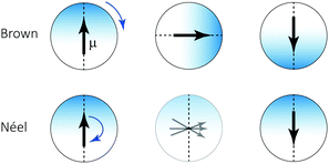
Magnetic nanoparticles (MNPs) possess fascinating properties that can be exploited in several engineering and biomedical applications.1–4 With typical diameters of their magnetic core on the order of 5–30 nm, MNPs are magnetic monodomain particles and therefore show “superparamagnetic” behavior.5 It is well-known that two basic mechanisms govern the magnetization relaxation of MNPs: (i) internal magnetization relaxation within the MNP, so-called Néel relaxation, on time scale τN, and (ii) so-called Brownian relaxation on time scale τB by rotational diffusion of the whole MNP when the particle is suspended in a viscous liquid (see Fig. 1). The relative contribution of Brownian and Néel relaxation is crucial for optimal use of MNPs in many technical as well as biomedical applications, such as hyperthermia.3,6 Therefore, methods for determining their relative importance are currently being explored, helping to find the optimal colloids for the given application.7,8 For ferrofluids, where MNPs are suspended in a non-magnetic carrier fluid, Rosensweig assumed that both relaxation processes occur independently so that the corresponding rates can be added up to yield an effective relaxation given by5| |  | (1) |
Eqn (1) is fundamental for ferrofluid research and is used in numerous textbooks and research articles (see e.g.ref. 9, 10 and references therein). However, one should bear in mind that eqn (1) was originally suggested for non-interacting MNPs in the absence of external fields.
 |
| | Fig. 1 Schematic of the two basic relaxation mechanisms. Brownian relaxation: entire particle including its magnetic moment μ rotates in fluid. Néel relaxation: direction of magnetic moment rotates within particle core. In the thermally activated regime considered here, deviations from the easy axis are energetically disfavored and short-lived and thus neglected in our implementation of the Néel relaxation dynamics. | |
Since τN grows almost exponentially with the magnetic volume of the nanoparticle, while τB grows only linearly with its hydrodynamic volume, different ratios τN/τB can be realized for core–shell particles with the same magnetic material by different sizes of the magnetic core and different thickness of the nonmagnetic shell (Section 2). The dependence of τB and τN on the strength of an external magnetic field has recently been determined experimentally by comparing the field-dependent magnetic susceptibility in the fluid and freeze-dried state for very dilute conditions.11 In another set of very recent experiments, the concentration dependence of the magnetization relaxation has been measured and the Brownian and Néel contributions have been identified.7 While the effective Brownian relaxation time was found to increase with increasing concentration, a weaker, opposite behavior was observed for the effective Néel relaxation time. Furthermore, the corresponding dynamic magnetic susceptibility deviates strongly from the Debye law for non-interacting MNPs and the effective relaxation time (1) is not sufficient to describe the behavior. Intriguingly, some experiments suggest that Brownian effects seem to play a role under conditions where only Néel relaxation was expected.12 In addition, hysteresis measurements pointed out the importance of dipolar interactions for magnetic losses that are relevant e.g. in hyperthermia applications.13
A number of computer simulation studies have investigated the magnetization dynamics when Brownian and Néel relaxation are both present. Few of these studies have thereby incorporated the stochastic Landau–Lifshitz–Gilbert (LLG) equation for a faithful representation of the internal magnetization dynamics14–16 as suggested by Shliomis and Stepanov.17,18 In the physically relevant regime where Néel relaxation is a rare, thermally activated process, the LLG approach is computationally very inefficient. Therefore, kinetic Monte-Carlo schemes have been used19,20 to simulate the magnetization response of frozen multi-core magnetic particles to oscillating fields. For ferrofluids, a Monte-Carlo scheme to equilibrate the magnetic moments alongside their translational diffusion was proposed.21 Recently, a diffusion-jump model was proposed to efficiently model internal Néel relaxation as a thermally activated jump process alongside the Brownian rotational diffusion of the MNPs.22 For non-interacting MNPs, good agreement with the underlying model of Shliomis and Stepanov was found over a reasonable range of model parameters.
However, since the magnetic properties of interacting MNPs are much less understood,23–25 we here address the question about the validity and form of eqn (1) for interacting MNPs. In ref. 25, concentration effects on the effective relaxation time in magnetorelaxometry were observed experimentally, but due to the lack of theoretical models were interpreted in terms of non-interacting particles. How do τB and τN depend on concentration and dipolar interaction strength? How meaningful is the distinction between Brownian and Néel relaxation in an interacting system? To answer these questions, we build on the model proposed in ref. 22 and perform extensive Brownian dynamics simulations of the translational and rotational dynamics of interacting dipolar particles coupled to thermally activated Néel relaxation processes for a broad range of concentrations and dipolar interaction strengths.
The paper is organized as follows. Section 2 provides formulation of the diffusion-jump model for interacting MNPs. Results of extensive computer simulations of this model are presented and analysed in Section 3. In particular, Sections 3.3 and 3.4 deal with the case that only Brownian and Néel relaxation is present, respectively. The corresponding models, denoted as brownian rigid dipole (RBD) model and frozen ferrofluid with Néel flip/magnetization reversal (FFMR) model, specified in Appendix B, are special cases of the full model (coupled case), for which results are presented in Section 3.4. Conclusions are offered in Section 4.
2 Model formulation
Consider a system of N interacting particles in a volume V corresponding to the number density n = N/V. Let ri and μi = μui denote the position and magnetic moment of particle i, respectively, where μ denotes the magnitude and ui the three-dimensional unit vector of the orientation of its magnetic moment. For simplicity we here consider monodisperse systems. To better represent experimental systems with significant polydispersity in nanoparticle sizes, generalizing the model is straightforward (e.g. along the lines of ref. 26).
The potential energy of the system in the presence of an external magnetic field H can be expressed as
| |  | (2) |
where
kB and
T are Boltzmann's constant and temperature, respectively. The spherically symmetric potential
Φs models steric repulsion. Following common practice,
27,28 we employ a purely repulsive Lennard-Jones potential,
| |  | (3) |
with
rij = |
ri −
rj| the distance between particles
i and
j,
rcut = 2
1/6σ, the interaction strength
ε and the Lennard-Jones diameter
σ as a measure for the spherical diameter of the particle. The dimensionless local field acting on particle
i is given by
| |  | (4) |
where
h =
μ0μH/
kBT denotes the dimensionless magnetic field,
λ =
μ0μ2/(4π
σ3kBT) the dimensionless strength of the dipole–dipole interaction relative to thermal energy, and
μ0 the permeability of free space. The equilibrium properties of system described by
eqn (2) depend strongly on
λ and the volume fraction
ϕ =
nπ
σ3/6.
29
In principle, eqn (2) should be supplemented by the magnetic anisotropy energy Kvm(ui·ni)2 due to deviations of the magnetic moment direction from the particle's easy axis orientation ni, where K is the anisotropy constant of the magnetic material and vm the volume of the magnetic core of the nanoparticle.10,18,30 Here, we consider MNPs that are sufficiently large with a correspondingly large magnetic anisotropy energy Kvm that magnetic moment and easy axis can be considered to be well-aligned. For iron oxide nanoparticles, K ≈ 104 J m−3, this means we consider magnetic core diameters larger than 12 nm, so that κ = Kvm/kBT ≳ 2 at room temperature, whereas for cobalt nanoparticles, K ≈ 2 × 10⁵ J m−3, already magnetic core diameters greater than 5 nm lead to κ ≳ 3. We note that experiments have confirmed that magnetization reversals of individual MNPs on the order of 15–30 nm are well-described by thermal activation over a single-energy barrier.31 We use this classical picture in the diffusion-jump model that we describe next.
Having defined the interaction potential, we also need to specify the dynamics of the system. We assume over-damped motion in a viscous carrier fluid of viscosity ηs with translational and rotational friction coefficients ξ and ξrot, respectively. The single particle Brownian diffusion time is given by τB = ξrot/2kBT with ξrot = πηsσ3, where ηs denotes the solvent viscosity. Let F(![[r with combining low line]](https://www.rsc.org/images/entities/b_char_0072_0332.gif) ,
,![[u with combining low line]](https://www.rsc.org/images/entities/b_char_0075_0332.gif) ;t) denote the probability density to find the position and magnetization orientation at time t, with the short notation
;t) denote the probability density to find the position and magnetization orientation at time t, with the short notation ![[r with combining low line]](https://www.rsc.org/images/entities/b_char_0072_0332.gif) = r1,…,rN,
= r1,…,rN, ![[u with combining low line]](https://www.rsc.org/images/entities/b_char_0075_0332.gif) = u1,…,uN. We propose the following model for the translational and rotational dynamics
= u1,…,uN. We propose the following model for the translational and rotational dynamics
| |  | (5) |
with the Fokker–Planck operator
| | 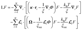 | (6) |
with
∇i ≡ ∂/∂
ri and the rotational operator

. The first and second line describe translational and rotational diffusion subject to the interaction potential
Φ and an imposed flow field with (transpose) velocity gradient
κ and (one-half) vorticity
Ω. Thus, the model reduces for
![[scr Q, script letter Q]](https://www.rsc.org/images/entities/char_e530.gif)
= 0 to the “rigid dipole model” (
τN → ∞) where Néel relaxation is fully suppressed and the magnetic moment is assumed to remain permanently fixed within the particle. The rigid dipole model is frequently used to study equilibrium and nonequilibrium dynamics
32 in ferrofluids.
The term ![[scr Q, script letter Q]](https://www.rsc.org/images/entities/char_e530.gif) in eqn (5) describes Néel relaxation as jump processes
in eqn (5) describes Néel relaxation as jump processes ![[u with combining low line]](https://www.rsc.org/images/entities/b_char_0075_0332.gif) →
→ ![[u with combining low line]](https://www.rsc.org/images/entities/b_char_0075_0332.gif) ′,
′,
| |  | (7) |
with transition rates
w. Equations of the type
(5) with
(6) and (7) are known in the literature as “differential Chapman–Kolmogorov” equations.
33 In order to complete the model, we therefore need to specify the transition rates
w in
eqn (7). We here follow
ref. 22 and assume sufficiently large magnetic anisotropy energies
κ that the magnetic moments are well-aligned with the particle's easy axis,
ui = ±
ni, so that the transition rates
w vanish unless
ui′ = −
ui. Assuming furthermore individual and statistically independent magnetization reversals,
![[u with combining low line]](https://www.rsc.org/images/entities/b_char_0075_0332.gif) (i)
(i) ≡
u1,…,
ui−1, −
ui,
ui+1…,
uN, we use the ansatz
| |  | (8) |
We ensure that the Boltzmann equilibrium
Feq ∼ exp[−
Φ/
kBT] is a stationary solution to the dynamics
(5),
i.e. ![[scr Q, script letter Q]](https://www.rsc.org/images/entities/char_e530.gif)
[
Feq] = 0, by the detailed balance condition
| |  | (9) |
Generalizing the model proposed in
ref. 22 to include dipolar interactions we choose
| | Λi(![[r with combining low line]](https://www.rsc.org/images/entities/b_char_0072_0332.gif) , ,![[u with combining low line]](https://www.rsc.org/images/entities/b_char_0075_0332.gif) ) = Λ0 ) = Λ0![[thin space (1/6-em)]](https://www.rsc.org/images/entities/char_2009.gif) exp[−ui·hi,loc], exp[−ui·hi,loc], | (10) |
which satisfies the detailed balance condition
(9) identically. Through the local field
hi,loc given by
eqn (4), the rates
Λi include dipolar interactions. Choosing the constant
Λ0 = 1/(2
τN) ensures the correct limit in the absence of external fields and dipolar interactions
22 (Appendix A). Our model can also be used to study the blocking temperature in relation to the field-cooled and zero-field cooled magnetization, extending previous studies on non-interacting MNPs.
34 Some authors found it necessary to include distributions of magnetic anisotropy constants, representing the energy barriers of individual particles.
12 This could be incorporated in the present model by a distribution of
Λ0 values. The dependence of the single-particle Néel relaxation time
τN on the anisotropy parameter
κ was already derived by Brown and reads

for
κ ≳ 2, where
τ0 is typically in the order of 10
−10–10
−9 s, usually two to four orders of magnitude smaller than
τN.
10 Therefore, by eliminating the time scale
τ0, our diffusion-jump model is orders of magnitude more efficient than approaches based on the LLG equation that need to resolve the fast internal magnetization dynamics on the time scale
τ0.
To summarize, the magnetic particles are specified by the dimensionless parameters λ and τB/τN, denoting the dipolar interaction parameter and the ratio of single-particle Brown and Néel relaxation times, respectively. The many-particle system is characterized by the amount and size of such magnetic particles, described by the volume fraction ϕ, and the strength of the steric repulsion given by ε = kBT.
3 Results and discussion
3.1 Simulation approach
To solve the coupled model described by eqn (5)–(10), we consider a time step Δt short enough so that the solution to eqn (5) can be approximated by| | F(t + Δt) ≈ eΔtLF(t) + Δt![[scr Q, script letter Q]](https://www.rsc.org/images/entities/char_e530.gif) [F(t)]. [F(t)]. | (11) |
For simplicity we used the short notation F(t) for the probability density F(![[r with combining low line]](https://www.rsc.org/images/entities/b_char_0072_0332.gif) ,
,![[u with combining low line]](https://www.rsc.org/images/entities/b_char_0075_0332.gif) ;t). The first term on the right hand side of eqn (11) represents Brownian translational and rotational motion described by the Fokker–Planck operator (6), whereas the second term describes magnetization reversals according to eqn (7)–(10). The numerical solution can therefore be broken up in two independent parts per time step: (i) Brownian dynamics simulations are employed to advance particles' positions and orientations for a time step Δt according to the translational and rotational Brownian motion (6). This step is identical to many previous simulation studies on ferrofluids that used the rigid-dipole approximation (see e.g.ref. 32 and references therein). (ii) A kinetic Monte-Carlo scheme to implement the jump processes described by
;t). The first term on the right hand side of eqn (11) represents Brownian translational and rotational motion described by the Fokker–Planck operator (6), whereas the second term describes magnetization reversals according to eqn (7)–(10). The numerical solution can therefore be broken up in two independent parts per time step: (i) Brownian dynamics simulations are employed to advance particles' positions and orientations for a time step Δt according to the translational and rotational Brownian motion (6). This step is identical to many previous simulation studies on ferrofluids that used the rigid-dipole approximation (see e.g.ref. 32 and references therein). (ii) A kinetic Monte-Carlo scheme to implement the jump processes described by ![[scr Q, script letter Q]](https://www.rsc.org/images/entities/char_e530.gif) [F]: (a) Select a dipole i at random and calculate the effective rate Λi = Λi(
[F]: (a) Select a dipole i at random and calculate the effective rate Λi = Λi(![[r with combining low line]](https://www.rsc.org/images/entities/b_char_0072_0332.gif) (t),
(t),![[u with combining low line]](https://www.rsc.org/images/entities/b_char_0075_0332.gif) (t)). (b) Flip the orientation of the magnetic dipole, ui → −ui, with probability p = 1 − e−ΔtΛi. (c) repeat steps (a) and (b) N times.
(t)). (b) Flip the orientation of the magnetic dipole, ui → −ui, with probability p = 1 − e−ΔtΛi. (c) repeat steps (a) and (b) N times.
Parts (i) and (ii) conclude one integration step time of length Δt. More details on the algorithm are given in Appendix B. This hybrid algorithm where Brownian dynamics and kinetic Monte-Carlo steps are alternated is similar to stochastic reaction-diffusion algorithms.33,35
The main quantity of interest in this study is the instantaneous magnetization which is defined as the total magnetic moment per unit volume,
| |  | (12) |
where we have defined the saturation magnetization
Msat =
Nμ/
V and the unit vector parallel to the external field direction
Ĥ. The reduced magnetization
U is defined by
U(
t) =
Ĥ·
M(
t)/
Msat.
Before discussing the validity and interpretation of eqn (1) for interacting magnetic nanoparticles, we first study the Brownian (RBD model) and Néel (FFMR model) relaxation separately in Sections 3.2 and 3.3, before addressing their combined effect (coupled model) in Section 3.4. To prevent confusion from the outset, we are going to use a unique notation (Table 1) for relaxation times occurring under different circumstances. The single particle relaxation times are the basic quantities determined by the nanoparticle and the solvent. Since dipolar interactions lead in general to non-exponential relaxation, we characterise the relaxation of the interacting system by the short-time behavior τshort and an effective, integrated relaxation time ![[small tau, Greek, macron]](https://www.rsc.org/images/entities/i_char_e0d4.gif) . We also fit the relaxation to a superposition of exponential decays with τn the relaxation time of mode n. Experimental data can be analyzed the same way. The various relaxation times are necessary to characterize the features of the full time-dependent signal in a compact fashion.
. We also fit the relaxation to a superposition of exponential decays with τn the relaxation time of mode n. Experimental data can be analyzed the same way. The various relaxation times are necessary to characterize the features of the full time-dependent signal in a compact fashion.
Table 1 Different relaxation times for the Brownian RBD (subscript B), Néelian FFMR (subscript N), and coupled models
|
|
RBD model |
FFMR model |
Coupled |
| Single particle |
τ
B
|
τ
N
|
τ
eff
|
| Short-time |
τ
B
|
τ
shortN
|
τ
short
|
| Mode n |
τ
B,n
|
τ
N,n
|
τ
n
|
| Effective |
![[small tau, Greek, macron]](https://www.rsc.org/images/entities/i_char_e0d4.gif) B
B
|
![[small tau, Greek, macron]](https://www.rsc.org/images/entities/i_char_e0d4.gif) N
N
|
![[small tau, Greek, macron]](https://www.rsc.org/images/entities/i_char_e0d4.gif)
|
3.2 Brownian relaxation for rigid dipoles (RBD model)
Computer simulation studies of ferrofluids frequently rely on the rigid-dipole approximation (RBD model), where Néel relaxation is completely ignored (τN → ∞).29,32,36–38 In this section, we study this model of interacting magnetic nanoparticles, UB(t), for a wide range of particle concentration and interaction strengths. Fig. 2 shows a selection of our computer simulation results for the magnetization relaxation after a strong ordering magnetic field has been switched off at time t = 0. Results for different volume fractions ϕ and dipolar interaction strengths λ are shown, corresponding to different values of the Langevin susceptibility χL = 8λϕ. We find from Fig. 2 that the magnetization relaxation deviates from a single-exponential behavior except for very weak interaction strengths. Therefore, we use the multi-mode ansatz| |  | (13) |
to fit our simulation data, where k = 2, 4,… denotes the number of parameters, τB,n denotes the relaxation time of mode n and cn the corresponding weight. Note that the relaxation spectrum {τB,n} can in principle be determined from the Laplace transform of the signal, where the shortest relaxation time captures the initial decay, while the longest relaxation time describes the exponential decay at long times. The short-time behavior is always given by the single-particle relaxation time, UB(t) = 1 − t/τB + ![[scr O, script letter O]](https://www.rsc.org/images/entities/char_e52e.gif) (t2). Therefore, we determine c0 and τB,0 from
(t2). Therefore, we determine c0 and τB,0 from  and
and  . In addition, we use the convention τB,n > τB,n+1 for n > 0 so that τB,1 denotes the longest relaxation time.
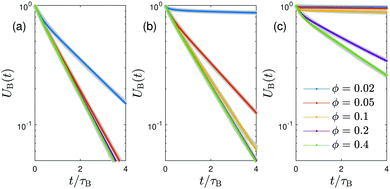 |
| | Fig. 2 RBD model. Magnetization relaxation UB(t), eqn (12) from a strongly magnetized initial state as a function of scaled time t/τB. The three panels correspond to Langevin susceptibilities (a) χL = 0.5, (b) 1 and (c) 5, respectively. In each panel, the concentration increases from top to bottom from ϕ = 0.02 to 0.4 as indicated in the legend. Measured data shown in gray, our fits using (13) with k according to Fig. 3 are colored. Fitted longest relaxation times τB,1 shown in Fig. 4. | |
Using a Bayesian information criterion (Appendix B.5 for further details), we determine the minimum number of parameters k in eqn (13) needed for a quantitative description of the magnetization relaxation data. Fig. 3 shows the result for k in the χL − ϕ parameter space. We observe that pronounced multi-mode relaxation is found for small concentrations and large values of χL, i.e. large dipolar interaction strengths λ.
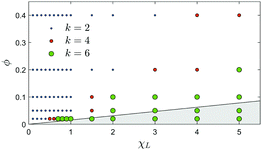 |
| | Fig. 3 RBD model. The minimum number of parameters k in the magnetization relaxation eqn (13) determined by a Bayesian information criterion for different points in the χL − ϕ parameter plane. The shaded gray area shows the regime λ > λfs with λfs = 8, corresponding to significant finite-size effects. | |
We use a cluster analysis in order to investigate structure formation in this system directly. Following earlier works,39,40 we define two particles to belong to the same cluster if their dipolar interaction energy is within 75% of the contact energy of two aligned dipoles. From the cluster analysis, we find that clusters start spanning the simulation box massively for large dipolar interaction strengths λ ≳ λfs with λfs = 8, whereas our results seem not to be significantly effected by finite-size effects for λ ≲ λfs.
Fitting our numerical results for the magnetization relaxation in the RBD model, Fig. 2, to the form (13), we obtain the effective Brownian relaxation times τB,n for a range of concentrations and interaction strengths. In Fig. 4, we show the longest effective Brownian relaxation times τB,1 normalized by the single-particle τB as a function of χL. For relatively weak interactions, we find that the increase of the longest effective relaxation time τB,1 is well described by the so-called first order modified-mean field model,41,42
| | | τMMFB,1 = τB(1 + χL/3) | (14) |
The derivation of
eqn (14) within mean-field theory is provided in Appendix C. Our findings are in good agreement with those of Sindt
et al.,
42 who found that
eqn (14) provides a good description up to
χL ≲ 1 for
λ ≲ 4. For stronger interactions,
Fig. 4 shows that the relaxation times grow significantly stronger than predicted by the modified mean-field model. This result is in qualitative agreement with earlier findings of slow relaxation processes in strongly interacting ferrofluids using the same rigid-dipole model.
36 We also note that the relaxation times are no longer a function of
χL alone, but depend on the volume fraction
ϕ and
λ separately. This finding is in line with predictions from cluster expansions for the magnetization
43 and magnetoviscosity.
44 As a word of caution, we estimate that finite-size effects for
λ >
λfs affect those data with
τB,1 ≳ 100
τB.
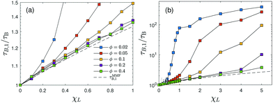 |
| | Fig. 4 RBD model. The longest effective Brownian relaxation time τB,1 normalized by the bare relaxation time τB as a function of the Langevin susceptibility χL (on a semilogarithmic scale). Dashed line shows the prediction of the modified mean-field model (14). Panel (a) is a zoom of panel (b) for small χL values. | |
Fig. 5 shows that the deviation of the relaxation time from the modified mean field prediction is a function of λ only and can be captured in the form
| |  | (15) |
where
a ≈ 40,
λc = 4.9 ± 0.5 and
z = 0.4 ± 0.1. The strong increase in the Brownian relaxation time beyond the modified mean-field prediction shown in
Fig. 5 and indicated by
eqn (15) suggests that major structure formation occurs in dilute systems for
λ ≳ 5. Our cluster analysis confirms this conclusion. In addition, this conclusion is also in line with previous computer simulations of various dipolar model systems that have established the formation of chains and rings in the dilute, strongly interacting regime.
29,45
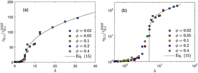 |
| | Fig. 5 RBD model. The longest Brownian relaxation time τB,1 scaled by the prediction τMMFB,1, eqn (14)versus dipolar interaction strength λ. Solid black line shows the approximation (15). Same data as shown in Fig. 4. Panel (a) shows the data on a linear, panel (b) in a double-logarithmic scale. | |
3.3 Néel relaxation for immobile particles (FFMR model)
In order to study the Néel relaxation process in isolation, we consider in this section immobile particles by suppressing Brownian motion completely (τB → ∞). For a better comparison, we start with the same initial conditions as used in Section 3.2, i.e. we first perform standard BD simulations in the presence of a strong ordering external field to prepare initial configurations. Once steady state is reached, at time t = 0 we instantaneously switch off the external field and run the FFMR model. The frozen particle configuration represents a quenched disorder and we later need to average our results over independently prepared equilibrium starting configurations. Such systems and the corresponding field-cooled magnetization have attracted considerable interest in the literature on solid magnetic materials and spin glasses due to slow relaxation processes.46,47 In view of biomedical applications, more studies on magnetic properties of immobile MNPs have appeared in recent years (see e.g. Zhao et al.16 for a simulation study on magnetization relaxation of non-interacting MNPs and Jonasson et al.20 where dipolar interactions within a multi-core particle are included).
Fig. 6 shows our FFMR model result for the relaxation of the reduced magnetization UN(t) = M(t)/Msat averaged over independent, frozen particle configurations from a strongly magnetized initial state. For weak interactions, we observe a single-exponential decay. Upon increasing the interaction strength χL and depending on volume fraction ϕ, we find both, the appearance of a remanent magnetization Mr = U∞Msat > 0, and two slightly different relaxation times, τshortN < ![[small tau, Greek, macron]](https://www.rsc.org/images/entities/i_char_e0d4.gif) N, where τshortN characterizes the initial decay of the magnetization. The appearance of a remanent magnetisation Mr in field-cooled magnetic systems at low temperatures has been observed experimentally.48 One expects Mr > 0.5Msat, i.e. U∞ > 0.5, for ferromagnetic interactions and Mr < 0.5Msat for anti-ferromagnetic interactions.46
N, where τshortN characterizes the initial decay of the magnetization. The appearance of a remanent magnetisation Mr in field-cooled magnetic systems at low temperatures has been observed experimentally.48 One expects Mr > 0.5Msat, i.e. U∞ > 0.5, for ferromagnetic interactions and Mr < 0.5Msat for anti-ferromagnetic interactions.46
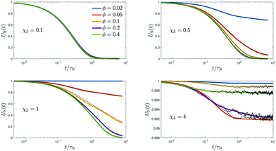 |
| | Fig. 6 FFMR model. Magnetization relaxation UN(t) averaged over 10 independent, frozen particle configurations from a strongly magnetized initial state as a function of reduced time t/τN for different ϕ. Each panel has its own χL value. Measured data (black) shown together with the approximant (16). Note the different range of UN values for the largest χL. A zoom into the short time window is provided in the appendix, Fig. 13. | |
We identify the short-time relaxation time τshortN (Fig. 7a) from our data (exemplarily shown in Fig. 6) by the inverse initial slope of d![[thin space (1/6-em)]](https://www.rsc.org/images/entities/char_2009.gif) ln
ln![[thin space (1/6-em)]](https://www.rsc.org/images/entities/char_2009.gif) UN/dt for times smaller than 0.05τN. The remaining characteristics U∞ and
UN/dt for times smaller than 0.05τN. The remaining characteristics U∞ and ![[small tau, Greek, macron]](https://www.rsc.org/images/entities/i_char_e0d4.gif) N are obtained reliably with τshortN at hand. Because more than two different relaxation times are not required to fit all our results with a relative deviation of less than 1% to an expression of the form (13) with k = 2 for U(t) − U∞, we use the ansatz
N are obtained reliably with τshortN at hand. Because more than two different relaxation times are not required to fit all our results with a relative deviation of less than 1% to an expression of the form (13) with k = 2 for U(t) − U∞, we use the ansatz
| | | UN(t) = U∞ + (c − U∞)e−t/τN,1 + (1 − c)e−t/τN,2 | (16) |
where
τN,2 =
τN,1τshortN(1 −
c)/[
τN,1 +
τshortN(
U∞ −
c)],
U∞ ∈ [0,1],
c ∈ [0,1] and
c −
U∞ ∈ [0,1]. With this unique choice for
τN,2,
eqn (16) exhibits by construction the four required features,
UN(0) = 1,
UN(
t) = 1 −
t/
τshortN +
O(
t2),

, as well as an exponential decrease at
t ≫
τN,1 ≥
τshortN that is governed by relaxation time
τN,1 in the absence of a remanent magnetization. An effective relaxation time
![[small tau, Greek, macron]](https://www.rsc.org/images/entities/i_char_e0d4.gif) N
N we determine uniquely, also in the presence of nonvanishing
U∞,
via| |  | (17) |
with
UN(
t) from
eqn (16) to capture the regime of times beyond simulation time. We thus have
![[small tau, Greek, macron]](https://www.rsc.org/images/entities/i_char_e0d4.gif) N
N = (
c −
U∞)
τN,1 + (1 −
c)
τN,2 using the parameters already obtained. Both, the resulting remanent
U∞ and effective relaxation time
![[small tau, Greek, macron]](https://www.rsc.org/images/entities/i_char_e0d4.gif) N
N, are shown
versus χL for various
ϕ in
Fig. 7b and c.
 |
| | Fig. 7 FFMR model. Quantities characterizing the magnetization dynamics in the absence of Brownian relaxation. The following quantities had been evaluated viaeqn (16) from the measured data: (a) inverse short relaxation time τshortN, (b) remanent reduced magnetization U∞, and (c) inverse effective Néel relaxation time ![[small tau, Greek, macron]](https://www.rsc.org/images/entities/i_char_e0d4.gif) N normalized by the bare relaxation time τN, all as a function of the Langevin susceptibility χL. Solid line in (a) and dashed line in (c) highlight predictions of the mean-field estimates (18) (ba = 1) and (19) (s = 1), respectively. N normalized by the bare relaxation time τN, all as a function of the Langevin susceptibility χL. Solid line in (a) and dashed line in (c) highlight predictions of the mean-field estimates (18) (ba = 1) and (19) (s = 1), respectively. | |
For weakly interacting systems (χL ≲ 0.5), we expect U∞ = 0 when starting with sufficiently random positions,30 whereas U∞ ≈ 0.5 was found in the low-temperature regime in an earlier study where particles occupy randomly the sites of a regular lattice for volume fractions ϕ < 0.5 and λ = 1.48 These authors found that dipolar interactions can lead to U∞ > 0 also in the high-temperature regime. Our FFMR model results (Fig. 7b) confirm these expectations, while U∞ quickly exceeds 0.5 with increasing χL. Beyond χL ≈ 3 all systems up to the largest volume fractions exhibit a remanent magnetization.
From Fig. 7a and c we find that the short time τshortN drops almost mono-exponentially with respect to χL, while the effective Néel relaxation time ![[small tau, Greek, macron]](https://www.rsc.org/images/entities/i_char_e0d4.gif) N decreases only approximately linearly with χL. The relaxation times approach unique curves with increasing concentration, i.e. decreasing λ. To understand these behaviors, we here offer simple mean-field arguments for (i) the short-time relaxation τshortN and (ii) the effective relaxation time
N decreases only approximately linearly with χL. The relaxation times approach unique curves with increasing concentration, i.e. decreasing λ. To understand these behaviors, we here offer simple mean-field arguments for (i) the short-time relaxation τshortN and (ii) the effective relaxation time ![[small tau, Greek, macron]](https://www.rsc.org/images/entities/i_char_e0d4.gif) N. From eqn (5)–(7), we find dUN/dt = −τN−1〈e−u·hlocuz〉t where UN(t) = 〈uz〉t and the local field hloc defined by eqn (4). Since we are dealing with an interacting many-particle system, we do not expect to find a closed-form solution to this equation, and thus treat problem (i) and (ii) using a mean-field approach.
N. From eqn (5)–(7), we find dUN/dt = −τN−1〈e−u·hlocuz〉t where UN(t) = 〈uz〉t and the local field hloc defined by eqn (4). Since we are dealing with an interacting many-particle system, we do not expect to find a closed-form solution to this equation, and thus treat problem (i) and (ii) using a mean-field approach.
(i) For the short-time relaxation from a strongly ordered initial state, we can use a factorization approximation 〈e−u·hlocuz〉t ≈ 〈e−u·hloc〉tUN(t). Together with a first-order cumulant expansion, we find dUN/dt ≈ −UN/τshortN with the short-time effective relaxation time τshortN = τNe〈u·hloc〉. To make further progress, we need to approximate the local field. For weak to moderate dipolar interactions, we adopt the modified mean-field model, hloc ≈ h + χL〈u〉.41 For strong interactions, we follow the chain-formation model49 and include in the local field only the contributions from a single, perfectly straight chain. Using in addition that UN ≈ 1 for short times, we arrive at the estimate
where
ba = 1 for weak and moderate dipolar interactions and
ba =
ζ/(4
ϕ) in the chain-forming regime, where
ζ defined in
eqn (44) depends weakly on the mean chain length (more details on the derivation can be found in the Appendix D). We observe that
eqn (18) describes the FFMR data in
Fig. 7a accurately for weak interactions and also explains qualitatively the behavior for stronger interactions.
(ii) Estimating the effective relaxation time ![[small tau, Greek, macron]](https://www.rsc.org/images/entities/i_char_e0d4.gif) N is more challenging. For weak dipolar interactions, we again use the modified mean-field approximation for hloc. We solve the differential equation for UN to first order in χL to arrive at the effective relaxation time
N is more challenging. For weak dipolar interactions, we again use the modified mean-field approximation for hloc. We solve the differential equation for UN to first order in χL to arrive at the effective relaxation time
| | τN/![[small tau, Greek, macron]](https://www.rsc.org/images/entities/i_char_e0d4.gif) N ≈ 1 − sχL N ≈ 1 − sχL | (19) |
with
s = 5/9. The corresponding calculation in the chain-formation regime leads to a more complicated expression, but might be approximated by
(19) with
s = 5
ζ/(36
ϕ). Details of the calculation are given in Appendix D. We emphasize that these theoretical estimates assume
U∞ = 0 and therefore apply only for moderate to strong but not too strong interactions. Comparing the prediction
(19) to
Fig. 7c, we find that the mean-field predictions are qualitatively correct. However, they are quantitatively less accurate than for the short-time regime.
Finally a word of caution on interpreting ![[small tau, Greek, macron]](https://www.rsc.org/images/entities/i_char_e0d4.gif) N, eqn (17), seems in order. While
N, eqn (17), seems in order. While ![[small tau, Greek, macron]](https://www.rsc.org/images/entities/i_char_e0d4.gif) N is well-defined also when U∞ > 0, its interpretation as an effective relaxation time becomes more and more questionable as U∞ increases. Therefore, we have omitted in Fig. 7c those data for which U∞ > 0.
N is well-defined also when U∞ > 0, its interpretation as an effective relaxation time becomes more and more questionable as U∞ increases. Therefore, we have omitted in Fig. 7c those data for which U∞ > 0.
3.4 Effective relaxation in coupled system
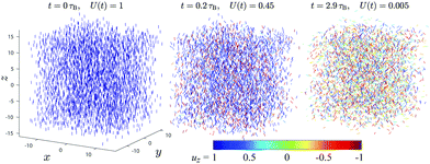
Having studied the effect of inter-particle interactions on Brownian and Néel relaxation via the RBD and FFMR models separately in Sections 3.2 and 3.3, we now investigate the fully coupled system where Brownian translational and rotational motion occurs simultaneously with Néel processes. As above, we equilibrate a number of statistically independent configurations in the presence of a strong external magnetic field. At t = 0, the field is turned off instantaneously and we follow the relaxation dynamics as described by the differential Chapman–Kolmogorov eqn (5). Snapshots of some particle configuration during relaxation are shown in Fig. 8.
 |
| | Fig. 8 Coupled model. Snapshots of particle configurations at different times during relaxation for N = 4000 particles, χL = 0.9, ϕ = 0.1, τN/τB = 0.1. The time t and corresponding reduced magnetization U(t) are indicated in each panel. The colour scheme encodes the projection of the magnetic moments on the direction of the orienting field (now switched off). | |
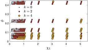 |
| | Fig. 9 Coupled model. The minimum number of parameters k in the magnetization relaxation eqn (21) determined by a Bayesian information criterion. Different points in the χL–ϕ–(τB/τN) parameter space are shown, where τB/τN – four values for each (χL,ϕ)-pair – increases from front to back. | |
The resulting relaxation behavior of the reduced magnetization U(t) as a function of time for selected parameter values is shown in Fig. 10. It shows some similarities with the corresponding Fig. 7 for the FFMR model. We now carefully analyse the data and perform a thorough comparison. From the inverse initial slope of ln![[thin space (1/6-em)]](https://www.rsc.org/images/entities/char_2009.gif) U(t) versus time t, we determine the effective short-time relaxation time τshort. The values obtained for τshort are shown in Fig. 11 as τeff/τshort versus χL for different volume fractions ϕ and different ratios τN/τB. For vanishing interactions, χL → 0, τshort becomes identical to the single-particle effective relaxation time τeff defined in eqn (1). Fig. 11 shows that dipolar interactions lead to a significant increase of τshort compared to τeff. We find that the mean-field prediction
U(t) versus time t, we determine the effective short-time relaxation time τshort. The values obtained for τshort are shown in Fig. 11 as τeff/τshort versus χL for different volume fractions ϕ and different ratios τN/τB. For vanishing interactions, χL → 0, τshort becomes identical to the single-particle effective relaxation time τeff defined in eqn (1). Fig. 11 shows that dipolar interactions lead to a significant increase of τshort compared to τeff. We find that the mean-field prediction
| |  | (20) |
describes this increase quite accurately for
ϕ ≳ 0.1. Details on the derivation of
eqn (20) are given in Appendix E. For more dilute systems, the mean-field prediction is accurate only for weak enough dipolar interactions but underpredicts
τshort for larger values of
λ. It is interesting to note that the Néel contribution to 1/
τshort vanishes for large
χL so that 1/
τshort → 1/
τB. These observations are very similar to the FFMR case when only Néel relaxation is present. Since we know from the RBD model that dipolar interactions do not affect the short-time relaxation when Néel processes are absent, we conclude that Brownian and Néel relaxation can be considered as independent processes at short times. Therefore, the effective short-time relaxation rate 1/
τshort is to a very good approximation the sum of the Brownian and Néel short-time relaxation rates.
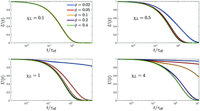 |
| | Fig. 10 Coupled model. The magnetization relaxation U(t) as a function of reduced time t/τeff for τB/τN = 1 (each panel has a different χL value). Measured data (black) together with our fits to eqn (21) using a Bayesian information criterion, see Appendix (B.5) and Fig. 9. Different panels correspond to different values of χL, with different volume fractions ϕ color-coded as indicated in the legend. | |
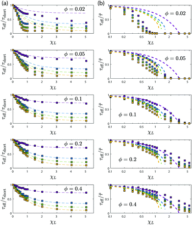 |
| | Fig. 11 Coupled model. The scaled, (a) inverse short-time relaxation time τeff/τshort and (b) inverse effective relaxation time τeff/![[small tau, Greek, macron]](https://www.rsc.org/images/entities/i_char_e0d4.gif) are shown versus the Langevin susceptibility χL for various volume fractions ϕ. In each panel τN increases from bottom to top: yellow, τN/τB = 0.1; green, τN/τB = 0.25; blue, τN/τB = 1.0; purple, τN/τB = 2.5. Dashed lines indicate the mean-field prediction (20) for τshort and (23) for are shown versus the Langevin susceptibility χL for various volume fractions ϕ. In each panel τN increases from bottom to top: yellow, τN/τB = 0.1; green, τN/τB = 0.25; blue, τN/τB = 1.0; purple, τN/τB = 2.5. Dashed lines indicate the mean-field prediction (20) for τshort and (23) for ![[small tau, Greek, macron]](https://www.rsc.org/images/entities/i_char_e0d4.gif) . . | |
Analysing the relaxation curves in Fig. 10 in more detail, we find that they can be described very accurately by a superposition of decaying exponentials,
| |  | (21) |
in the same form as in the RBD case,
eqn (13). Indeed, the data (in black) are indistinguishable on the scale of the plot from the fit (in color) in
Fig. 10. Note that for weak interactions,
χL = 0.1, results for different volume fractions
ϕ superimpose on the same curve. For larger
χL, however, this is no longer the case and smaller
ϕ corresponding to larger
λ lead to slower relaxation. We determine the minimum number of parameters
k needed in the fits shown in
Fig. 10 from a Bayesian information criterion (Appendix B.5). In
Fig. 9, we show the results for the minimum number of parameters
k needed in the fits for the coupled system. For sufficiently weak interactions, we find
k = 0,
i.e. a single-exponential relaxation. In this case, the relaxation time has already been identified above from the short-time behavior. We find that additional modes of relaxation are needed for stronger interactions in a very similar manner as for the RBD model (
Fig. 3). Interestingly, for most points in the
χL–
ϕ plane, different values of
τB/
τN do not change the number of modes needed for an accurate fit.
Since the interpretation of the longest relaxation time in a multi-mode fit can be unclear when the corresponding weight is small, we define an effective relaxation time for the coupled system analogue to eqn (17) as
| |  | (22) |
Note that Brownian relaxation enforces
U∞ = 0. Definition
(22) of
![[small tau, Greek, macron]](https://www.rsc.org/images/entities/i_char_e0d4.gif)
we find to be very useful and robust.
Fig. 11b shows the inverse of
![[small tau, Greek, macron]](https://www.rsc.org/images/entities/i_char_e0d4.gif)
scaled with the single-particle effective relaxation time
τeff,
eqn (1). Since our fits to
U(
t) are very accurate, we evaluate
![[small tau, Greek, macron]](https://www.rsc.org/images/entities/i_char_e0d4.gif)
from
eqn (22) as

using the fit values of
τn and
cn. We observe from
Fig. 11 a that dipolar interactions lead to a strong increase in
![[small tau, Greek, macron]](https://www.rsc.org/images/entities/i_char_e0d4.gif)
that, contrary to the short-time relaxation, does not level off at large
χL. We find from
Fig. 11b that the mean-field prediction for
![[small tau, Greek, macron]](https://www.rsc.org/images/entities/i_char_e0d4.gif)
,
| |  | (23) |
is not as accurate as the one for
τshort, but provides a good description for weak and moderate interaction strengths.
Eqn (23) holds for
χL < 3 and (
χL − 1)
τB <
τN and we have defined
τMF =
τeff/(1 −
χL/3) and
b1 =
χL(
τN − 2
τB)/[(3 −
χL)(
τN +
τB)]. Details on the derivation of
eqn (23) are given in Appendix E. For stronger interactions, mean-field theory predicts a vanishing rate 1/
![[small tau, Greek, macron]](https://www.rsc.org/images/entities/i_char_e0d4.gif)
at some critical value of
χL, whereas the simulations show a gradual decrease, deviating from the mean-field predictions earlier the larger
λ.
The effective relaxation time ![[small tau, Greek, macron]](https://www.rsc.org/images/entities/i_char_e0d4.gif) increases with χL as shown in Fig. 12a on a linear scale. Interestingly, a stronger increase of
increases with χL as shown in Fig. 12a on a linear scale. Interestingly, a stronger increase of ![[small tau, Greek, macron]](https://www.rsc.org/images/entities/i_char_e0d4.gif) relative to the non-interacting τeff is seen when compared to the relative increase of τB,1 relative to τB obtained using the RBD model (Fig. 4). For small enough χL, this increase of
relative to the non-interacting τeff is seen when compared to the relative increase of τB,1 relative to τB obtained using the RBD model (Fig. 4). For small enough χL, this increase of ![[small tau, Greek, macron]](https://www.rsc.org/images/entities/i_char_e0d4.gif) is well described by the mean-field result (23). For smaller ϕ corresponding to larger dipolar interaction strength λ, the data start to diverge earlier from the mean-field result. In order to better analyse deviations from the mean-field result, Fig. 12b shows the effective relaxation time
is well described by the mean-field result (23). For smaller ϕ corresponding to larger dipolar interaction strength λ, the data start to diverge earlier from the mean-field result. In order to better analyse deviations from the mean-field result, Fig. 12b shows the effective relaxation time ![[small tau, Greek, macron]](https://www.rsc.org/images/entities/i_char_e0d4.gif) , eqn (22), scaled with the mean-field prediction (61)versus the dipolar interaction parameter λ. As mentioned above, the mean-field result (23) predicts a divergence of
, eqn (22), scaled with the mean-field prediction (61)versus the dipolar interaction parameter λ. As mentioned above, the mean-field result (23) predicts a divergence of ![[small tau, Greek, macron]](https://www.rsc.org/images/entities/i_char_e0d4.gif) at sufficiently strong interactions, but (61) provides a good approximation for χL < 1. Therefore, we consider in Fig. 12b the mean-field result (61) which does not diverge but is accurate up to second order in χL only. From Fig. 12b, we observe an S-shaped curve, where the mean-field result holds quite well for small λ, but seriously underestimates the simulation results for larger λ. We also note that data collapse is encouraging, even though not as good as in the case where only Brownian relaxation is present, Fig. 5. The onset of the strong increase of
at sufficiently strong interactions, but (61) provides a good approximation for χL < 1. Therefore, we consider in Fig. 12b the mean-field result (61) which does not diverge but is accurate up to second order in χL only. From Fig. 12b, we observe an S-shaped curve, where the mean-field result holds quite well for small λ, but seriously underestimates the simulation results for larger λ. We also note that data collapse is encouraging, even though not as good as in the case where only Brownian relaxation is present, Fig. 5. The onset of the strong increase of ![[small tau, Greek, macron]](https://www.rsc.org/images/entities/i_char_e0d4.gif) /
/![[small tau, Greek, macron]](https://www.rsc.org/images/entities/i_char_e0d4.gif) MF occurs around λ ≈ 5, very similar to our RBD model observations. Therefore, an improved theory for Brownian relaxation in strongly interacting systems is very likely to lead to correspondingly improved predictions also in the coupled case.
MF occurs around λ ≈ 5, very similar to our RBD model observations. Therefore, an improved theory for Brownian relaxation in strongly interacting systems is very likely to lead to correspondingly improved predictions also in the coupled case.
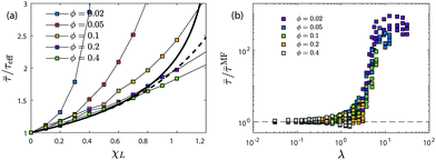 |
| | Fig. 12 Coupled model. (a) Reduced effective relaxation time ![[small tau, Greek, macron]](https://www.rsc.org/images/entities/i_char_e0d4.gif) (22)versus χL for various ϕ and τN/τB = 1/4, up to χL = 1. Results are quite insensitive to the precise value of τN. Both the mean field result (23) (thick solid black) and its expansion (61) (dashed black) are shown for comparison. The mean field expression is not able to capture data for χL > 1 well. (b) The effective relaxation time (22)versus χL for various ϕ and τN/τB = 1/4, up to χL = 1. Results are quite insensitive to the precise value of τN. Both the mean field result (23) (thick solid black) and its expansion (61) (dashed black) are shown for comparison. The mean field expression is not able to capture data for χL > 1 well. (b) The effective relaxation time ![[small tau, Greek, macron]](https://www.rsc.org/images/entities/i_char_e0d4.gif) scaled with the second-order mean-field prediction (61)versus the dimensionless dipolar interaction strength λ. Data for all available χL, ϕ and τN/τB values are shown. Black dashed line indicates the mean-field prediction (61). scaled with the second-order mean-field prediction (61)versus the dimensionless dipolar interaction strength λ. Data for all available χL, ϕ and τN/τB values are shown. Black dashed line indicates the mean-field prediction (61). | |
3.5 Magnetic susceptibility for coupled system
Measurements of the dynamic magnetic susceptibility ![[small chi, Greek, tilde]](https://www.rsc.org/images/entities/i_char_e11b.gif) (ω) are more common than magnetization relaxation experiments U(t). From a theoretical point of view, these quantities are related by
(ω) are more common than magnetization relaxation experiments U(t). From a theoretical point of view, these quantities are related by ![[small chi, Greek, tilde]](https://www.rsc.org/images/entities/i_char_e11b.gif) (ω) = χ0[1 − iω
(ω) = χ0[1 − iω![[C with combining tilde]](https://www.rsc.org/images/entities/i_char_0043_0303.gif) (iω)], where χ0 denotes the static susceptibility and
(iω)], where χ0 denotes the static susceptibility and  the Laplace-transform of the magnetization fluctuation C(t) = 〈u(t)·u(0)〉. Thanks to the fluctuation–dissipation theorem, we can identify C(t) with the relaxation function U(t). We note that by definition
 ![[C with combining tilde]](https://www.rsc.org/images/entities/i_char_0043_0303.gif) (0) =
(0) = ![[small tau, Greek, macron]](https://www.rsc.org/images/entities/i_char_e0d4.gif) and therefore the low-frequency behavior is given by
and therefore the low-frequency behavior is given by ![[small chi, Greek, tilde]](https://www.rsc.org/images/entities/i_char_e11b.gif) (ω) = χ0[1 − iω
(ω) = χ0[1 − iω![[small tau, Greek, macron]](https://www.rsc.org/images/entities/i_char_e0d4.gif) +
+ ![[scr O, script letter O]](https://www.rsc.org/images/entities/char_e52e.gif) (ω2)], i.e. governed by the effective relaxation time defined in eqn (22).
(ω2)], i.e. governed by the effective relaxation time defined in eqn (22).
For the coupled system, we have seen in Section 3.4 that the relaxation is very well described by a weighted sum of exponentials, eqn (21). Using this form, we evaluate the real and imaginary part of the dynamic susceptibility, ![[small chi, Greek, tilde]](https://www.rsc.org/images/entities/i_char_e11b.gif) = χ′ − iχ′′ as
= χ′ − iχ′′ as
| |  | (24) |
| |  | (25) |
From
Fig. 9, we find only a small parameter region with
k = 0, corresponding to the classical Debye model. In the rest of the parameter space, however, dipolar interactions lead to a multi-mode relaxation and corresponding deviations from the simple Debye behavior. The multi-mode nature of the magnetic susceptibility prohibits the unique definition of a single characteristic relaxation time from
χ′′. Similar difficulties are encountered in interpreting the non-exponential magnetization relaxation. While defining an effective relaxation time from relaxation measurements
viaeqn (22) is common, many authors identify relaxation times with peaks in
χ′′. While this approach has been used to identify Brownian and Néel relaxation times when those processes happen on well separated time scales,
7,8 our results show that such a separation runs into problems when dipolar interactions are present and time scales are not well separated, since the individual
τn already contain Brownian and Néel contributions.
4 Conclusions and outlook
With the current work, we provide a comprehensive study of the effective magnetization dynamics of interacting magnetic nanoparticles in solution when Brownian and Néel processes are both present. We perform extensive computer simulation studies using Brownian Dynamics coupled with Monte-Carlo methods of magnetization reversals to simulate the magnetization relaxation after a strong ordering field is switched off.
First, we study Brownian (RBD model, Section 3.2) and Néel (FFMR model, Section 3.3) contributions separately, before considering the coupled case when both processes are active (Section 3.4). In all three cases, we find that dipolar interactions lead to deviations from a single-exponential decay. Therefore, a careful analysis of the data is required. For the RBD model we find that the short-time relaxation is unaffected by dipolar interactions, whereas in the other cases, the effective short-time relaxation time increases. We propose a mean-field argument that captures this increase rather well. The long-time or integrated effective relaxation time is found to increase due to dipolar interactions in all our simulations. Using the RBD model we confirm earlier findings that the increase in the long-time relaxation time is well described by the modified mean-field theory for weak to moderate interaction strengths.42 We also show that corrections to this result for stronger interactions should be sought in terms of the dipolar interaction strength λ, rather than χL. For Néel relaxation in the absence of Brownian motion (FFMR model), we propose a mean-field argument to explain the increase of the effective relaxation time. We note that an earlier study found that dipolar interactions reduce rather than increase the Néel relaxation time.50 However, in the latter work, the authors consider CoPt core–shell nanoparticles that are compressed into dense conglomerates. Therefore, it would be interesting to extend our studies to higher volume fractions to find out conditions under which the effective Néel relaxation would be enhanced due to dipolar interactions.
When Brownian and Néel processes are both present (coupled model), we find that the corresponding rates from the RBD and FFMR model are in general not additive for interacting systems. Accordingly, equations of the form (1) hold only for very weak dipolar interactions. A noteworthy exception is the short-time relaxation, ln![[thin space (1/6-em)]](https://www.rsc.org/images/entities/char_2009.gif) U(t) = −t/τshort +
U(t) = −t/τshort + ![[scr O, script letter O]](https://www.rsc.org/images/entities/char_e52e.gif) (t2) for t → 0, where the coupled rate 1/τshort is well described as the sum of the short time RBD and FFMR rates. Therefore, in interacting systems, Brownian and Néel relaxation can be considered as independent processes for very short times only. Since our findings apply also to magnetic susceptibility spectra, their interpretation is challenging when the single particle Brownian and Néel relaxation times are comparable.
(t2) for t → 0, where the coupled rate 1/τshort is well described as the sum of the short time RBD and FFMR rates. Therefore, in interacting systems, Brownian and Néel relaxation can be considered as independent processes for very short times only. Since our findings apply also to magnetic susceptibility spectra, their interpretation is challenging when the single particle Brownian and Néel relaxation times are comparable.
We note that our study explored the regime 0.1 ≤ τN/τB ≤ 10. For larger values of τN/τB, the rigid-dipole approximation becomes more and more accurate. In the opposite limit of dominant Néel relaxation, τN ≪ τB, pronounced two-step relaxation was observed experimentally in ref. 7. This regime is left for future research.
Finally, we want to emphasize that the coupled model studied here of combining Brownian translational and rotational dynamics with Néel-type magnetization reversals can be simulated very efficiently. The efficiency relies on modeling the Néel process as thermally activated magnetization reversals via Monte-Carlo methods. This physically appealing picture underlies also Brown's classical treatment (see e.g.ref. 10 and references therein). It breaks down, however, for particles with sufficiently small magnetic core, where the energy barriers for deviations of the particle's magnetic moment from their easy axis (anisotropy energy) become equal to or even smaller than the thermal energy. In the latter case, the internal magnetization dynamics should rather be simulated with the stochastic LLG equation. While the stochastic approach is considered to provide a more faithful representation of the internal magnetization dynamics, this model becomes very inefficient for ferrofluids containing magnetic nanoparticles with large anisotropy energies. Therefore, we propose our model to susbstitute the LLG approach in the physically relevant regime of large anisotropy barriers where magnetization reversals can be modelled as thermally activated events. It is well-suited for studying further, e.g. field-dependent properties of interacting ferrofluids.
Conflicts of interest
There are no conflicts to declare.
A Néel contribution to magnetization relaxation
In terms of the probability density F(![[r with combining low line]](https://www.rsc.org/images/entities/b_char_0072_0332.gif) ,
,![[u with combining low line]](https://www.rsc.org/images/entities/b_char_0075_0332.gif) ;t), the time-dependent magnetization is defined by eqn (12). Using eqn (5), the magnetization dynamics can be expressed as
;t), the time-dependent magnetization is defined by eqn (12). Using eqn (5), the magnetization dynamics can be expressed as| |  | (26) |
where  and the first and second term describe the contribution due to Brownian dynamics and Néel relaxation, respectively. For the present modeling of Néel relaxation by eqn (7) and (8), we find for the contribution of dipole i
| |  | (27) |
where we made use of a change of integration variables from ![[u with combining low line]](https://www.rsc.org/images/entities/b_char_0075_0332.gif) to
to ![[u with combining low line]](https://www.rsc.org/images/entities/b_char_0075_0332.gif) (j) and
(j) and ![[u with combining low line]](https://www.rsc.org/images/entities/b_char_0075_0332.gif) (i) for j ≠ i and j = i, respectively. In the absence of external fields and dipolar interactions (of particular relevance for the FFMR model), we find from eqn (10) that Λi reduces to Λ0 = 1/(2τN) and eqn (27) leads to a contribution −M/τN to the magnetization relaxation.
(i) for j ≠ i and j = i, respectively. In the absence of external fields and dipolar interactions (of particular relevance for the FFMR model), we find from eqn (10) that Λi reduces to Λ0 = 1/(2τN) and eqn (27) leads to a contribution −M/τN to the magnetization relaxation.
B Implementation of RBD, FFMR, and coupled model
All three parts of our algorithm to be described below (orientation-BD, translation-BD, flip-MC) can be independently switched on or off, which allows us to prepare the conditions required for the various ‘experiments’, and to define three models. The frozen ferrofluid with Néel flip/magnetization reversal (FFMR model) uses the flip-MC part only. The Brownian rigid dipole (RBD model) uses orientation and translation BD only. The full BD + MC algorithm including all parts is denoted as coupled model.
For a sphere of diameter σ, the Brownian translational and rotational friction coefficients are respectively given by ξ = 3πηsσ and ξrot = πηsσ3 with solvent viscosity ηs. We use the Brownian rotational relaxation time τB = ξrot/2kBT to introduce reduced units. For a system with given ϕ and rRF and periodic box size ≥2rRF = 16σ for our choice of rRF, the number of particles must exceed 48ϕrRF3/πσ3 ≈ 7823ϕ. In this section we omit all units σ, ε and τB, as they do not appear in the algorithm.
B.1 Orientation-BD
The orientational Brownian dynamics corresponding to ![[u with combining dot above]](https://www.rsc.org/images/entities/b_char_0075_0307.gif) i = (ωi + Ẇ) × ui with
i = (ωi + Ẇ) × ui with  and Wiener process W reads, using the abbreviation ai = hloci,y
![[thin space (1/6-em)]](https://www.rsc.org/images/entities/char_2009.gif) cos
cos![[thin space (1/6-em)]](https://www.rsc.org/images/entities/char_2009.gif) ϕi − hloci,x
ϕi − hloci,x![[thin space (1/6-em)]](https://www.rsc.org/images/entities/char_2009.gif) sin
sin![[thin space (1/6-em)]](https://www.rsc.org/images/entities/char_2009.gif) ϕi,
ϕi,| |  | (28) |
with a time step Δt, and reflecting boundary conditions for zi ∈ [−1,1]. The ΔW's are independent random numbers with 〈ΔW2〉 = Δt. The constraints |ui| = 1 are taken care of automatically, as we switched to spherical coordinates to represent ui by an angle ϕi and its zi-component. We use equally distributed random numbers ζ ∈ [0,1] and  to generate them. Calculations are done using the reaction-field approximation with metallic boundary conditions, which amounts to replacing hloci by
  in eqn (28). Several test of the above algorithm were performed, checking e.g. the correct stationary magnetization and rotational diffusion in the non-interacting case.
B.2 Translation-BD
The translational Brownian dynamics corresponding to  is governed by
| |  | (29) |
with| |  | (30) |
and rik = ri − rk, rik = |rik|, ![[r with combining circumflex]](https://www.rsc.org/images/entities/b_char_0072_0302.gif) = r/r, where the components of ΔW are all independent random numbers with 〈ΔW2〉 = Δt, and generated as in Section B.1. The sum in (29) does not run over all k ≠ i. For the first term λGik it runs over all k with rik ≤ rRF. The second LJ part involves only terms with rik ≤ rcut = 21/6. We verified the correct translational diffusion in the non-interacting case.
= r/r, where the components of ΔW are all independent random numbers with 〈ΔW2〉 = Δt, and generated as in Section B.1. The sum in (29) does not run over all k ≠ i. For the first term λGik it runs over all k with rik ≤ rRF. The second LJ part involves only terms with rik ≤ rcut = 21/6. We verified the correct translational diffusion in the non-interacting case.
B.3 Flip-MC
As has been noted in ref. 22, the ansatz (10) can be generalized to| | Λi(![[r with combining low line]](https://www.rsc.org/images/entities/b_char_0072_0332.gif) , ,![[u with combining low line]](https://www.rsc.org/images/entities/b_char_0075_0332.gif) ) = Λ0r(|xi|)exp[−xi] ) = Λ0r(|xi|)exp[−xi] | (31) |
with xi = ui·hi,loc which satisfies the detailed balance condition (9) identically for all choices of functions r with r > 0 and r(0) = 1. Note that the choice r = 1 lead to Arrhenius-like expression (10), whereas r(x) = sech(x) leads to Glauber-like rates of the form Λi = (2τN)−1[1 + tanh(−x)]. Also the phenomenological expression r(x) = cosh(ax) has been considered22 with parameter 0 ≤ a ≤ 1.
We use a Monte-Carlo scheme to implement this jump process. At each time step Δt, every magnetic moment is flipped with its individual probability pi = 1 − exp(−ΔtΛi) with Λi = Λ0r(|xi|)exp(−xi) and xi = ui·hloci, where hloci is the same local field appearing in eqn (28), and thus already available at no additional computation cost. If not otherwise stated, r(x) = 1 is used. For the non-interacting case, we verified the equilibrium fluctuations satisfy 〈u1(t)·u1(0)〉 = e−t/τN.
B.4 Orientation relaxation ‘experiments’
To measure the effective orientational relaxation time, starting from a state of fully saturated magnetization M = μez that is realized in the limit h → ∞, we prepared equilibrated systems with initial ∀izi = 1 in the presence of translation-BD only. At time t = 0 we set h = 0 and either continue running using the FFMR, the RBD, or the coupled model. In each case we measure the decorrelation function 〈〈ui·ez〉〉(t) = M(t)·ez/Msat ≡ U(t), where the average is taken not only over all particles i, but also an ensemble of equilibrated initial configurations. The saturation magnetization is defined by Msat = nμ with n = N/V the number density.
The limiting case of noninteracting particles, or χL → 0, we study using many particles upon switching off the translation-BD and setting λ = 0. Under these conditions each of the three cases (i)–(iii) is characterized by a monoexponential decay (U∞ = 0), with the following relaxation times (i) ![[small tau, Greek, macron]](https://www.rsc.org/images/entities/i_char_e0d4.gif) N(Λ0) = τN, (ii)
N(Λ0) = τN, (ii) ![[small tau, Greek, macron]](https://www.rsc.org/images/entities/i_char_e0d4.gif) B = τB, and (iii) we confirm that U(t) = exp(−t/τeff) with τeff defined in eqn (1). The result can be considered trivial as the rotation-BD and flip-MC are completely independent in the absence of interactions, and because there is no reason for a trapped orientation.
B = τB, and (iii) we confirm that U(t) = exp(−t/τeff) with τeff defined in eqn (1). The result can be considered trivial as the rotation-BD and flip-MC are completely independent in the absence of interactions, and because there is no reason for a trapped orientation.
For the remaining results to presented we investigated 300 different systems with all combinations of χL ∈ {0.1, 0.2,…, 0.9, 1, 1.5, 2, 3, 4, 5}, ϕ ∈ {0.02, 0.05, 0.1, 0.2, 0.4}, and Λ0 ∈ {0.2, 1, 2, 5} or τN ∈ {2.5, 1, 0.25, 0.1}, implying λ's to reside within the range λ ∈ [0.03, 31]. For each set of parameters we run all three models, and evaluated UN(t), UB(t), U(t), as well as the corresponding characteristic times ![[small tau, Greek, macron]](https://www.rsc.org/images/entities/i_char_e0d4.gif) N, τB,1, τB,2, τ1, τ2, and coefficients cB, c, and U∞.
N, τB,1, τB,2, τ1, τ2, and coefficients cB, c, and U∞.
B.5 Multi-exponential fitting of the relaxation function
In this section, we deal with the problem of how to characterize the region in the three-dimensional (ϕ − χL − τN/τB) parameter space where relaxation is monoexponential to a good approximation. For each system we measured N data points (ti,Ui) with uncertainties σi and we have competing fits Ufit(t) with several exponentials. For the FFMR model, cf.eqn (16), containing k = 4 (or less) parameters: τN,1, τN,2, U∞, c. For the RBD and coupled model, cf.eqn (13) and (21) with parameters {τB,n,cn} and {τn,cn}, respectively. For each of those fit functions, we define the corresponding quantities| |  | (32) |
where U∞ ≠ 0 occurs only in case of the FFMR model. Since uncertainties σi in our data do not vary significantly, they do not appear in eqn (32).
We generally expect fits with larger number of parameters k to be more accurate than with lower k. But to decide whether the double- or multi-exponential fit is preferable or rather overfitting the data, we employ the Bayesian information criterion (BIC) defined by
| | BICk = Nχk2 + k![[thin space (1/6-em)]](https://www.rsc.org/images/entities/char_2009.gif) ln ln![[thin space (1/6-em)]](https://www.rsc.org/images/entities/char_2009.gif) N N | (33) |
We conclude that the
k-parametric fit is appropriate if BIC
k is the smallest of all BIC's.
We find that for the RBD model the short-time behavior is always given by the single particle τB. Therefore, dipolar interactions lead to a multi-exponential decay with two (k = 2), three (k = 4) or four (k = 6) modes, see Fig. 3. For the FFMR model, the decay is monoexponential for k = 1, monoexponential with offset for k = 2, double-exponential without offset for k = 3, and k = 4 is found to be irrelevant by its BIC value. In the coupled case, we find a single-exponential regime (k = 0) as well as superposition of two (k = 2) and three (k = 4) exponentials, see Fig. 9.
C Mean-field arguments for RBD relaxation
C.1 Short-time RBD dynamics
Consider the magnetization dynamics (26) in the absence of Néel relaxation,| |  | (34) |
Using the modified mean-field approximation,41 we approximate the local field by hloc ≈ h + χL〈u〉. Let n denote the orientation of the ordering field. We assume that the magnetization remains parallel to n during the relaxation where the field has been switched off, 〈u〉 = UBn. Assuming furthermore uniaxial symmetry, 〈uu〉 = S2nn + (1 − S2)I/3, where I denotes the three-dimensional unit matrix, we can rewrite eqn (34) as| |  | (35) |
where S2 = 〈P2(u·n)〉 and P2(x) = (3x2 − 1)/2 denotes the second Legendre polynomial. Starting from a strongly oriented initial state, UB ≈ S2 ≈ 1, we find from eqn (35) that the short-time relaxation is given by the bare single-particle Brownian relaxation time, τB, i.e. remains unaffected by interparticle interactions.
C.2 Effective RBD relaxation time
For longer times, eqn (35) predicts a non-exponential decay due to the time-dependence of S2. Using a simple closure approximation S2 ≈ UB2, we arrive at the ordinary differential equation τb![[U with combining dot above]](https://www.rsc.org/images/entities/i_char_0055_0307.gif) B + UB = −bUB3, where
B + UB = −bUB3, where| |  | (36) |
and b = χL/[3 − χL]. The solution of this differential equation to the initial condition UB(0) = 1 reads| |  | (37) |
From eqn (37), we recover the short-time behavior UB = 1 − t/τB + ![[scr O, script letter O]](https://www.rsc.org/images/entities/char_e52e.gif) (t2) for t ≪ τb and an exponential decay for long times governed by τb. Note that eqn (37) agrees to first order in χL with the mean-field result for the RBD model, τMMFB,1 = τB(1 + χL/3), eqn (14). Our mean-field arguments therefore confirm the result (14) derived earlier. It should be noted that no expansion in χL was used in the derivation of eqn (37) and therefore the result is expected to hold in the whole regime where the modified mean-field approximation and the closure relation S2 ≈ UB2 apply.
(t2) for t ≪ τb and an exponential decay for long times governed by τb. Note that eqn (37) agrees to first order in χL with the mean-field result for the RBD model, τMMFB,1 = τB(1 + χL/3), eqn (14). Our mean-field arguments therefore confirm the result (14) derived earlier. It should be noted that no expansion in χL was used in the derivation of eqn (37) and therefore the result is expected to hold in the whole regime where the modified mean-field approximation and the closure relation S2 ≈ UB2 apply.
Defining an effective relaxation time  , we find from (37) for small χL
| |  | (38) |
Since the linear term is quite close to the mean-field result for the long-time relaxation,
τMMFB,1, the longest and the effective relaxation times agree quite well for small
χL.
D Mean-field arguments for FFMR relaxation
Let n denote the direction of the external field with which the system was prepared and UN(t) = 〈u·n〉t the time-dependent scaled magnetization. Point of departure is the magnetization dynamics (26) and (27), in the absence of Brownian motion,| |  | (39) |
D.1 Short-time FFMR dynamics
Fig. 13 shows the initial magnetization relaxation UN(t) when Brownian relaxation is absent. For the short-time dynamics, the system remains in the vicinity of the highly oriented initial state. Therefore, we use a factorization approximation| |  | (40) |
Inserting eqn (40) into (39) and using a cumulant expansion, we arrive at| |  | (41) |
with τN/τshortN = 〈e−u·hloc〉t = e−κ1+κ2/2+…, where the first cumulants are defined by κ1 = 〈u·hloc〉t, κ2 = 〈(u·hloc)2〉t − 〈u·hloc〉t2.
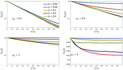 |
| | Fig. 13 FFMR model. Initial magnetization relaxation UN(t) averaged over 10 independent, frozen particle configurations from a strongly magnetized initial state as a function of reduced time t/τN for different χL and ϕ. Measured data (black) shown together with the approximant (16). Note the different range of UN values for the largest χL. | |
In order to evaluate the cumulants, we need to specify the local field. In the regime of weak up to moderate dipolar interactions, we use the modified mean-field model41 where hloc ≈ h + χL〈u〉. After the field is switched off, this expression becomes hloc = χLUNn. With this, the cumulants can be evaluated, κ1 = χLUN2 and κ2 = χL2UN2[2S2 − UN + 1]/3, where S2 = 〈P2(u·n)〉 and P2 denotes the second Legendre polynomial. For short times where the magnetic moments are still strongly aligned, UN ≈ S2 ≈ 1, we find κ1 ≈ χL and κ2 ≈ 0 and therefore
| | | τN/τshortN ≈ e−χL, λ ≲ 1 | (42) |
For stronger dipolar interactions, the modified mean-field model fails due to significant chain formation. In this regime, we follow the chain-formation model49 and assume that the local field can be approximated by the contributions from neighboring particles within a single, perfectly straight chain,
| |  | (43) |
Assuming furthermore that all particles in the chain are still oriented in direction of the ordering field (which is now switched off),
uj =
n, we find that we can approximate the local field contribution as
u·
hloc ≈ 2
λζ(
u·
n)
2, where
| |  | (44) |
and the average is performed over all particles
i in the chain. We note that
ζ is monotonously increasing with increasing chain length and reaches its asymptotic value 2
ζ(3) ≈ 2.404 for infinite chain lengths. With this approximation for the chain-formation regime, the cumulants can be evaluated to give
κ1 = 2
λζ[1 + 2
S2]/3 and
| |  | (45) |
For short times where the magnetic moments are still strongly aligned,
S4 ≈
S2 ≈ 1, we find
κ1 ≈ 2
λζ and
κ2 ≈ 0 so that
| | | τN/τshortN ≈ e−2λζ, 1 ≲ λ ≲ 5 | (46) |
With the definition of the Langevin susceptibility
χL = 8
λϕ, we can rewrite this expression in the form
(18) with
ba =
ζ/(4
ϕ).
D.2 Effective FFMR relaxation time
D.2.1 Moderate dipolar interactions.
In order to estimate the effective relaxation time (17) of the FFMR model, we want to first derive its magnetization relaxation UN(t) as predicted with the help of the modified mean-field approximation. Our starting point is the magnetization relaxation eqn (39) for weak dipolar interactions,| |  | (47) |
Truncating at first order in χL and assuming the simple closure approximation S2(t) ≈ UN2(t), we arrive at the nonlinear differential equation τa![[U with combining dot above]](https://www.rsc.org/images/entities/i_char_0055_0307.gif) N + UN = aUN3, with the long-time relaxation time τa = τN/(1 − χL/3) and a = 2χL/(3 − χL). Obviously, the range of validity of the approximation (47) is restricted to χL < 3. The solution to this differential equation for the initial condition UN(0) = 1 reads
N + UN = aUN3, with the long-time relaxation time τa = τN/(1 − χL/3) and a = 2χL/(3 − χL). Obviously, the range of validity of the approximation (47) is restricted to χL < 3. The solution to this differential equation for the initial condition UN(0) = 1 reads| |  | (48) |
For long times, t ≫ (τa/2), we indeed find an exponential decay governed by τa, UN ∼ e−t/τa. For short times, t ≪ τa, we find from eqn (48)
with the short-time relaxation τshortN = τN/(1 − χL). From eqn (48), we find that the magnetization relaxation deviates stronger from a single-exponential decay the larger χL becomes.
With UN(t) from eqn (48) at hand, we calculate the effective relaxation time from eqn (17),  , to find
| |  | (49) |
with
| |  | (50) |
and where the last equality holds when
a ∈ [0,1]. Since
φ(
a) = 1 +
a/3 +
a2/5 +
![[scr O, script letter O]](https://www.rsc.org/images/entities/char_e52e.gif)
(
a3) for
a → 0, we find that for weak dipolar interactions
| |  | (51) |
D.2.2 Chain-formation regime.
In order to estimate the effective relaxation time in the chain-formation regime of the FFMR model, we assume that the factorization approximation (40) remains valid during the whole relaxation process. Therefore, we consider| |  | (52) |
where we truncated the cumulant expansion after the first term with| |  | (53) |
Inserting κ1 into (52) and using the same closure approximation S2 ≈ UN2 as we did for moderate dipolar interactions, we arrive at a closed ordinary differential equation for UN, τα(dUN/dt) = −exp(−αUN2)UN, where τα = τN![[thin space (1/6-em)]](https://www.rsc.org/images/entities/char_2009.gif) exp[(2/3)λζ] and α = 4λζ/3. The solution for UN(t) can only be given in implicit form as
exp[(2/3)λζ] and α = 4λζ/3. The solution for UN(t) can only be given in implicit form as| |  | (54) |
where Ei(x) is the exponential integral. From eqn (54), we find the effective relaxation time by a change of integration variables as| |  | (55) |
where erfi(x) denotes the imaginary error function. For very strong dipolar interactions, λ → ∞, this expression becomes ![[small tau, Greek, macron]](https://www.rsc.org/images/entities/i_char_e0d4.gif) N ≈ τN3e2λζ/(8λζ), whereas in the opposite limit
N ≈ τN3e2λζ/(8λζ), whereas in the opposite limit  . Thus, we might approximate the corresponding relaxation rate in the form of eqn (19) with (10/9)ζλ = sχL or s = 5ζ/(36ϕ). Note, however, that the chain-formation model does not apply for too small values of λ and therefore we expect s = 5ζ/(36ϕ) to overpredict the observed relaxation rate.
E Mean-field arguments for relaxation in the coupled system
E.1 Short-time dynamics
Consider now the magnetization dynamics (26) when both, Brownian and Néel relaxation is present. Combining the corresponding expressions for the RBD and FFMR models (Appendices C and D) for the regime of weak to moderate interactions, where the modified mean-field approximation can be applied, we arrive at| |  | (56) |
From eqn (56), we find that the short-time relaxation (where S2 ≈ 1) is governed by the weighted sum of the RBD and FFMR individual particle rates,| |  | (57) |
Eqn (57) was derived for the case of weak to moderate interactions. We have seen above that eqn (42) provides a better description for the short-time FFMR contribution for larger values of χL. Assuming independent Brownian and Néel contributions to the short-time relaxation, we propose to generalise eqn (57) to| |  | (58) |
E.2 Effective relaxation time
In order to describe the full time evolution, we once again employ the simple closure approximation S2 ≈ U2. With this approximation, eqn (56) can be brought into the form τMF![[U with combining dot above]](https://www.rsc.org/images/entities/i_char_0055_0307.gif) + U = −b1U3, where
+ U = −b1U3, where| |  | (59) |
and τeff denotes the effective relaxation time for isolated particles, 1/τeff = 1/τB + 1/τN. The coefficient b1 is given by b1 = χLτMF(1/τB − 2/τN)/3. Since the time evolution equation is formally identical to the one encountered for the RBD model, we find the same functional form for the magnetisation relaxation,| |  | (60) |
This U(t) exhibits an exponential relaxation with τMF at long times (t ≫ τMF) and a short-time regime with U(t) = 1 − t/τMFshort + ![[scr O, script letter O]](https://www.rsc.org/images/entities/char_e52e.gif) (t2). Eqn (60) implies, for χL < 3 and (χL − 1)τB < τN, that the effective relaxation time defined in eqn (22) is given by eqn (23), where for negative b1 the expression can be rewritten with the identity tan−1(ix) = i
(t2). Eqn (60) implies, for χL < 3 and (χL − 1)τB < τN, that the effective relaxation time defined in eqn (22) is given by eqn (23), where for negative b1 the expression can be rewritten with the identity tan−1(ix) = i![[thin space (1/6-em)]](https://www.rsc.org/images/entities/char_2009.gif) tanh−1(x). For weak interactions we find from eqn (23)
tanh−1(x). For weak interactions we find from eqn (23)| |  | (61) |
with u1 = [(2/9)τN + (5/9)τB]/(τN + τB) and u2 = (8τN2 + 28τNτB + 47τB2)/[135(τN + τB)2]. Therefore, to second order in χL we find| |  | (62) |
Note that equation reduces for τB → ∞ to the FFMR model (61), and for τN → ∞ to the result (38) we obtained for the RBD model.
F Dynamic magnetic susceptibility
In order to calculate the dynamic magnetic susceptibility, we first need to find the Laplace-transform of the relaxation function. Using the mean-field result for the coupled system (60), or similarly (48) for the FFMR model, we find| | 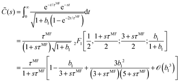 | (63) |
with the hypergeometric function 2F1 in the 2nd line. Inserting this expression into ![[small chi, Greek, tilde]](https://www.rsc.org/images/entities/i_char_e11b.gif) (ω) = χ0[1 − iω
(ω) = χ0[1 − iω![[C with combining tilde]](https://www.rsc.org/images/entities/i_char_0043_0303.gif) (iω)], we find
(iω)], we find ![[small chi, Greek, tilde]](https://www.rsc.org/images/entities/i_char_e11b.gif) = χ′ − iχ′′ with
= χ′ − iχ′′ with| |  | (64) |
| |  | (65) |
up to second order in b1. For ease of notation, we defined the reduced frequency y = ωτMF. It is interesting to note that the mean-field model predicts deviations from the Debye model not in terms of additional Debye modes, but in the above form, with τMF, eqn (59) as basic time scale. The whole ![[small chi, Greek, tilde]](https://www.rsc.org/images/entities/i_char_e11b.gif) (ω) behavior is available from the second line of eqn (63), including its low and high frequency characteristics, but the coefficients of an expansion in terms of ω cannot be obtained in closed analytic form; they are available numerically. From eqn (61), we verify that the low-frequency behavior χ′′(ω) = χ0
(ω) behavior is available from the second line of eqn (63), including its low and high frequency characteristics, but the coefficients of an expansion in terms of ω cannot be obtained in closed analytic form; they are available numerically. From eqn (61), we verify that the low-frequency behavior χ′′(ω) = χ0![[small tau, Greek, macron]](https://www.rsc.org/images/entities/i_char_e0d4.gif) MFω +
MFω + ![[scr O, script letter O]](https://www.rsc.org/images/entities/char_e52e.gif) (ω3) is governed by the effective relaxation time
(ω3) is governed by the effective relaxation time ![[small tau, Greek, macron]](https://www.rsc.org/images/entities/i_char_e0d4.gif) MF, consistent with its definition.
MF, consistent with its definition.
Acknowledgements
M. K. acknowledges support by the Swiss National Science Foundation through grant 200021L_185052 and we thank the Swiss National Supercomputing Centre for providing computational resources.
Notes and references
- I. Torres-Diaz and C. Rinaldi, Recent progress in ferrofluids research: novel applications of magnetically controllable and tunable fluids, Soft Matter, 2014, 10, 8584–8602 RSC.
- L. Mohammed, H. G. Gomaa, D. Ragab and J. Zhu, Magnetic nanoparticles for environmental and biomedical applications: A review, Particuology, 2017, 30, 1–14 CrossRef CAS.
- Q. A. Pankhurst, N. T. K. Thanh, S. K. Jones and J. Dobson, Progress in applications of magnetic particles in biomedicine, J. Phys. D: Appl. Phys., 2009, 42, 224001 CrossRef.
- V. Uskoković, S. Tang and V. M. Wu, Targeted magnetic separation of biomolecules and cells using earthicle-based ferrofluids, Nanoscale, 2019, 11, 11236–11253 RSC.
-
R. E. Rosensweig, Ferrohydrodynamics, Cambridge University Press, Cambridge, 1985 Search PubMed.
- D. Shi, M. E. Sadat, A. W. Dunn and D. B. Mast, Photo-fluorescent and magnetic properties of iron oxide nanoparticles for biomedical applications, Nanoscale, 2015, 7, 8209–8232 RSC.
- S. Ota and Y. Takemura, Characterization of Néel and Brownian Relaxations Isolated from Complex Dynamics Influenced by Dipole Interactions in Magnetic Nanoparticles, J. Phys. Chem. C, 2019, 123, 28859–28866 CrossRef.
- L. Maldonado-Camargo, I. Torres-Diaz, A. Chiu-Lam, M. Hernández and C. Rinaldi, Estimating the contribution of Brownian and Néel relaxation in a magnetic fluid through dynamic magnetic susceptibility measurements, J. Magn. Magn. Mater., 2016, 412, 223–233 CrossRef CAS.
-
Colloidal Magnetic Fluids, ed. S. Odenbach, Springer, Berlin, 2009, vol. 763 Search PubMed.
-
E. Blums, A. Cebers and M. M. Maiorov, Magnetic Fluids, de Gruyter, Berlin, 1997 Search PubMed.
- J. Dieckhoff, D. Eberbeck, M. Schilling and F. Ludwig, Magnetic-field dependence of Brownian and Néel relaxation times, J. Appl. Phys., 2016, 119, 043903 CrossRef.
- S. A. Shah, D. B. Reeves, R. M. Ferguson, J. B. Weaver and K. M. Krishnan, Mixed Brownian alignment and Néel rotations in superparamagnetic iron oxide nanoparticle suspensions driven by an ac field, Phys. Rev. B, 2015, 92, 094438 CrossRef.
- S. Ota, T. Yamada and Y. Takemura, Dipole-dipole interaction and its concentration dependence of magnetic fluid evaluated by alternating current hysteresis measurement, J. Appl. Phys., 2015, 117, 17D713 CrossRef.
- H. Rogge, M. Erbe, T. M. Buzug and K. Lüdtke-Buzug, Simulation of the magnetization dynamics of diluted ferrofluids in medical applications, Biomed. Eng., 2013, 58, 1–9 Search PubMed.
- P. Ilg, Equilibrium magnetization and magnetization relaxation of multicore magnetic nanoparticles, Phys. Rev. B, 2017, 95, 214427 CrossRef.
- Z. Zhao, N. Garraud, D. P. Arnold and C. Rinaldi, Effects of particle diameter and magnetocrystalline anisotropy on magnetic relaxation and magnetic particle imaging performance of magnetic nanoparticles, Phys. Med. Biol., 2020, 65, 025014 CrossRef CAS.
- M. Shliomis and V. Stepanov, Rotational viscosity of magnetic fluids: contribution of the Brownian and Néel relaxational processes, J. Magn. Magn. Mater., 1993, 122, 196–199 CrossRef CAS.
-
M. Shliomis and V. Stepanov, in Relaxation Phenomena in Condensed Matter, ed. W. Coffey, John Wiley & Sons, 1994, vol. LXXXVII of Advances in Chemical Physics, pp. 1–30 Search PubMed.
- S. Ruta, R. Chantrell and O. Hovorka, Unified model of hyperthermia via hysteresis heating in systems of interacting magnetic nanoparticles, Sci. Rep., 2015, 5, 9090–9097 CrossRef CAS.
- C. Jonasson, V. Schaller, L. Zeng, E. Olsson, C. Frandsen, A. Castro, L. Nilsson, L. K. Bogart, P. Southern, Q. A. Pankhurst, M. Puerto Morales and C. Johansson, Modelling the effect of different core sizes and magnetic interactions inside magnetic nanoparticles on hyperthermia performance, J. Magn. Magn. Mater., 2019, 477, 198–202 CrossRef CAS.
- D. V. Berkov, N. L. Gorn and D. Stock, Combined Langevin dynamics/Monte-Carlo simulations of the non-equilibrium ferrofluid remagnetization, J. Magn. Magn. Mater., 2004, 272, E1281–E1283 CrossRef.
- P. Ilg, Diffusion-jump model for the combined Brownian and Néel relaxation dynamics of ferrofluids in the presence of external fields and flow, Phys. Rev. E, 2019, 100, 022608 CrossRef CAS.
- C. Iacovita, J. Hurst, G. Manfredi, P. A. Hervieux, B. Donnio, J. L. Gallani and M. V. Rastei, Magnetic force fields of isolated small nanoparticle clusters, Nanoscale, 2020, 12, 1842–1851 RSC.
- K. Wu, D. Su, R. Saha, J. Liu and J.-P. Wang, Investigating the effect of magnetic dipole–dipole interaction on magnetic particle spectroscopy: implications for magnetic nanoparticle-based bioassays and magnetic particle imaging, J. Phys. D: Appl. Phys., 2019, 52, 335002 CrossRef CAS.
- D. Eberbeck and L. Trahms, Experimental investigation of dipolar interaction in suspensions of magnetic nanoparticles, J. Magn. Magn. Mater., 2011, 323, 1228–1232 CrossRef CAS.
- P. J. Camp, E. A. Elfimova and A. O. Ivanov, The effects of polydispersity on the initial susceptibilities of ferrofluids, J. Phys.: Condens. Matter, 2014, 26, 456002 CrossRef.
- J. D. Weeks, D. Chandler and H. Andersen, Role of repulsive forces in determining the equilibrium structure of simple liquids, J. Chem. Phys., 1971, 54, 5237–5247 CrossRef CAS.
- S. Hess, M. Kröger and H. Voigt, Thermo-mechanical properties of the WCA-Lennard-Jones model system in its fluid and solid states, Physica A, 1998, 250, 58–82 CrossRef CAS.
- C. Holm and J. J. Weis, The structure of ferrofluids: A status report, Curr. Opin. Colloid Interface Sci., 2005, 10, 133–140 CrossRef CAS.
- E. A. Elfimova, A. O. Ivanov and P. J. Camp, Static magnetization of immobilized, weakly interacting, superparamagnetic nanoparticles, Nanoscale, 2019, 11, 21834–21846 RSC.
- W. Wernsdorfer, E. B. Orozcho, K. Hasselbach, A. Benoit, B. Barbara, N. Demoncy, A. Loiseau, H. Pascard and D. Mailly, Experimental Evidence of the Néel-Brown Model of Magnetization Reversal, Phys. Rev. Lett., 1997, 78, 1791–1794 CrossRef CAS.
-
P. Ilg and S. Odenbach, in Colloidal Magnetic Fluids: Basics, Development and Applications of Ferrofluids, ed. S. Odenbach, Springer, Berlin, 2008, vol. 763 of Lecture Notes in Physics, pp. 245–315 Search PubMed.
-
C. Gardiner, Stochastic Methods, Springer-Verlag, Berlin, Heidelberg, 2009 Search PubMed.
- K. L. Livesey, S. Ruta, N. R. Anderson, D. Baldomir, R. W. Chantrell and D. Serantes, Beyond the blocking model to fit nanoparticle ZFC/FC magnetisation curves, Sci. Rep., 2018, 8, 1–9 CrossRef CAS.
-
R. Erban, J. Chapman and P. Maini, A practical guide to stochastic simulations of reaction-diffusion processes, 2007, arxiv.org, arXiv:0704.1908v2.
- A. Sreekumari and P. Ilg, Slow relaxation in structure-forming ferrofluids, Phys. Rev. E, 2013, 88, 042315 CrossRef.
- G. Mériguet, M. Jardat and P. Turq, Brownian dynamics investigation of magnetization and birefringence relaxations in ferrofluids, J. Chem. Phys., 2005, 123, 144915 CrossRef.
- J. Jordanovic, S. Jaeger and S. H. L. Klapp, Crossover from Normal to Anomalous Diffusion in Systems of Field-Aligned Dipolar Particles, Phys. Rev. Lett., 2011, 106, 038301 CrossRef.
- Z. Wang, C. Holm and H. W. Müller, Molecular dynamics study on the equilibrium magnetization properties and structure of ferrofluids, Phys. Rev. E, 2002, 66, 021405 CrossRef.
- P. Ilg and M. Kröger, Anisotropic Self-Diffusion in Ferrofluids studied via Brownian Dynamics Simulations, Phys. Rev. E, 2005, 72, 031504 CrossRef.
- A. F. Pshenichnikov, V. V. Mekhonoshin and A. Lebedev, Magneto-granulometric analysis of concentrated ferrocolloids, J. Magn. Magn. Mater., 1996, 161, 94–102 CrossRef CAS.
- J. O. Sindt, P. J. Camp, S. S. Kantorovich, E. A. Elfimova and A. O. Ivanov, Influence of dipolar interactions on the magnetic susceptibility spectra of ferrofluids, Phys. Rev. E, 2016, 93, 063117 CrossRef.
- B. Huke and M. Lücke, Magnetization of ferrofluids with dipolar interactions: A Born-Mayer expansion, Phys. Rev. E, 2000, 62, 6875–6890 CrossRef CAS.
- P. Ilg and S. Hess, Nonequilibrium Dynamics and Magnetoviscosity of Moderately Concentrated Magnetic Liquids: A dynamic Mean-field Study, Z. Naturforsch., 2003, 58a, 589–600 Search PubMed.
- L. Rovigatti, J. Russo and F. Sciortino, Structural properties of the dipolar hard-sphere fluid at low temperatures and densities, Soft Matter, 2012, 8, 6310–6319 RSC.
- W. Luo, S. R. Nagel, T. F. Rosenbaum and R. E. Rosensweig, Dipole interactions with random anisotropy in a frozen ferrofluid, Phys. Rev. Lett., 1991, 67, 2721–2724 CrossRef CAS.
- S. Bedanta, S. Sahoo, X. Chen, W. Kleemann, D. Sudfeld, K. Wojczykowski and A. Hütten, Intra- and interparticle interaction in a dense frozen ferrofluid, Phase Transform., 2005, 78, 121–129 CrossRef CAS.
- D. Kechrakos and K. N. Trohidou, Magnetic properties of dipolar interacting single-domain particles, Phys. Rev. B, 1998, 58, 12169–12177 CrossRef CAS.
- A. Y. Zubarev and L. Y. Iskakova, Effect of chainlike aggregates on dynamical properties of magnetic liquids, Phys. Rev. E, 2000, 61, 5415–5421 CrossRef CAS.
- H. Kesserwan, G. Manfredi, J. Y. Bigot and P. A. Hervieux, Magnetization reversal in isolated and interacting single-domain nanoparticles, Phys. Rev. B, 2011, 84, 172407 CrossRef.
|
| This journal is © the Owner Societies 2020 |
Click here to see how this site uses Cookies. View our privacy policy here.  Open Access Article
 *a and
Martin
Kröger
 b
b


![[r with combining low line]](https://www.rsc.org/images/entities/b_char_0072_0332.gif) ,
,![[u with combining low line]](https://www.rsc.org/images/entities/b_char_0075_0332.gif) ;t) denote the probability density to find the position and magnetization orientation at time t, with the short notation
;t) denote the probability density to find the position and magnetization orientation at time t, with the short notation ![[r with combining low line]](https://www.rsc.org/images/entities/b_char_0072_0332.gif) = r1,…,rN,
= r1,…,rN, ![[u with combining low line]](https://www.rsc.org/images/entities/b_char_0075_0332.gif) = u1,…,uN. We propose the following model for the translational and rotational dynamics
= u1,…,uN. We propose the following model for the translational and rotational dynamics

 . The first and second line describe translational and rotational diffusion subject to the interaction potential Φ and an imposed flow field with (transpose) velocity gradient κ and (one-half) vorticity Ω. Thus, the model reduces for
 ![[scr Q, script letter Q]](https://www.rsc.org/images/entities/char_e530.gif) = 0 to the “rigid dipole model” (τN → ∞) where Néel relaxation is fully suppressed and the magnetic moment is assumed to remain permanently fixed within the particle. The rigid dipole model is frequently used to study equilibrium and nonequilibrium dynamics32 in ferrofluids.
= 0 to the “rigid dipole model” (τN → ∞) where Néel relaxation is fully suppressed and the magnetic moment is assumed to remain permanently fixed within the particle. The rigid dipole model is frequently used to study equilibrium and nonequilibrium dynamics32 in ferrofluids.
![[scr Q, script letter Q]](https://www.rsc.org/images/entities/char_e530.gif) in eqn (5) describes Néel relaxation as jump processes
in eqn (5) describes Néel relaxation as jump processes ![[u with combining low line]](https://www.rsc.org/images/entities/b_char_0075_0332.gif) →
→ ![[u with combining low line]](https://www.rsc.org/images/entities/b_char_0075_0332.gif) ′,
′,
![[u with combining low line]](https://www.rsc.org/images/entities/b_char_0075_0332.gif) (i) ≡ u1,…,ui−1, −ui, ui+1…,uN, we use the ansatz
(i) ≡ u1,…,ui−1, −ui, ui+1…,uN, we use the ansatz
![[scr Q, script letter Q]](https://www.rsc.org/images/entities/char_e530.gif) [Feq] = 0, by the detailed balance condition
[Feq] = 0, by the detailed balance condition
![[r with combining low line]](https://www.rsc.org/images/entities/b_char_0072_0332.gif) ,
,![[u with combining low line]](https://www.rsc.org/images/entities/b_char_0075_0332.gif) ) = Λ0
) = Λ0![[thin space (1/6-em)]](https://www.rsc.org/images/entities/char_2009.gif) exp[−ui·hi,loc],
exp[−ui·hi,loc], for κ ≳ 2, where τ0 is typically in the order of 10−10–10−9 s, usually two to four orders of magnitude smaller than τN.10 Therefore, by eliminating the time scale τ0, our diffusion-jump model is orders of magnitude more efficient than approaches based on the LLG equation that need to resolve the fast internal magnetization dynamics on the time scale τ0.
![[scr Q, script letter Q]](https://www.rsc.org/images/entities/char_e530.gif) [F(t)].
[F(t)].![[r with combining low line]](https://www.rsc.org/images/entities/b_char_0072_0332.gif) ,
,![[u with combining low line]](https://www.rsc.org/images/entities/b_char_0075_0332.gif) ;t). The first term on the right hand side of eqn (11) represents Brownian translational and rotational motion described by the Fokker–Planck operator (6), whereas the second term describes magnetization reversals according to eqn (7)–(10). The numerical solution can therefore be broken up in two independent parts per time step: (i) Brownian dynamics simulations are employed to advance particles' positions and orientations for a time step Δt according to the translational and rotational Brownian motion (6). This step is identical to many previous simulation studies on ferrofluids that used the rigid-dipole approximation (see e.g.ref. 32 and references therein). (ii) A kinetic Monte-Carlo scheme to implement the jump processes described by
;t). The first term on the right hand side of eqn (11) represents Brownian translational and rotational motion described by the Fokker–Planck operator (6), whereas the second term describes magnetization reversals according to eqn (7)–(10). The numerical solution can therefore be broken up in two independent parts per time step: (i) Brownian dynamics simulations are employed to advance particles' positions and orientations for a time step Δt according to the translational and rotational Brownian motion (6). This step is identical to many previous simulation studies on ferrofluids that used the rigid-dipole approximation (see e.g.ref. 32 and references therein). (ii) A kinetic Monte-Carlo scheme to implement the jump processes described by ![[scr Q, script letter Q]](https://www.rsc.org/images/entities/char_e530.gif) [F]: (a) Select a dipole i at random and calculate the effective rate Λi = Λi(
[F]: (a) Select a dipole i at random and calculate the effective rate Λi = Λi(![[r with combining low line]](https://www.rsc.org/images/entities/b_char_0072_0332.gif) (t),
(t),![[u with combining low line]](https://www.rsc.org/images/entities/b_char_0075_0332.gif) (t)). (b) Flip the orientation of the magnetic dipole, ui → −ui, with probability p = 1 − e−ΔtΛi. (c) repeat steps (a) and (b) N times.
(t)). (b) Flip the orientation of the magnetic dipole, ui → −ui, with probability p = 1 − e−ΔtΛi. (c) repeat steps (a) and (b) N times.

![[small tau, Greek, macron]](https://www.rsc.org/images/entities/i_char_e0d4.gif) . We also fit the relaxation to a superposition of exponential decays with τn the relaxation time of mode n. Experimental data can be analyzed the same way. The various relaxation times are necessary to characterize the features of the full time-dependent signal in a compact fashion.
. We also fit the relaxation to a superposition of exponential decays with τn the relaxation time of mode n. Experimental data can be analyzed the same way. The various relaxation times are necessary to characterize the features of the full time-dependent signal in a compact fashion.![[small tau, Greek, macron]](https://www.rsc.org/images/entities/i_char_e0d4.gif) B
B
![[small tau, Greek, macron]](https://www.rsc.org/images/entities/i_char_e0d4.gif) N
N
![[small tau, Greek, macron]](https://www.rsc.org/images/entities/i_char_e0d4.gif)

![[scr O, script letter O]](https://www.rsc.org/images/entities/char_e52e.gif) (t2). Therefore, we determine c0 and τB,0 from
(t2). Therefore, we determine c0 and τB,0 from  and
and  . In addition, we use the convention τB,n > τB,n+1 for n > 0 so that τB,1 denotes the longest relaxation time.


![[small tau, Greek, macron]](https://www.rsc.org/images/entities/i_char_e0d4.gif) N, where τshortN characterizes the initial decay of the magnetization. The appearance of a remanent magnetisation Mr in field-cooled magnetic systems at low temperatures has been observed experimentally.48 One expects Mr > 0.5Msat, i.e. U∞ > 0.5, for ferromagnetic interactions and Mr < 0.5Msat for anti-ferromagnetic interactions.46
N, where τshortN characterizes the initial decay of the magnetization. The appearance of a remanent magnetisation Mr in field-cooled magnetic systems at low temperatures has been observed experimentally.48 One expects Mr > 0.5Msat, i.e. U∞ > 0.5, for ferromagnetic interactions and Mr < 0.5Msat for anti-ferromagnetic interactions.46
![[thin space (1/6-em)]](https://www.rsc.org/images/entities/char_2009.gif) ln
ln![[thin space (1/6-em)]](https://www.rsc.org/images/entities/char_2009.gif) UN/dt for times smaller than 0.05τN. The remaining characteristics U∞ and
UN/dt for times smaller than 0.05τN. The remaining characteristics U∞ and ![[small tau, Greek, macron]](https://www.rsc.org/images/entities/i_char_e0d4.gif) N are obtained reliably with τshortN at hand. Because more than two different relaxation times are not required to fit all our results with a relative deviation of less than 1% to an expression of the form (13) with k = 2 for U(t) − U∞, we use the ansatz
N are obtained reliably with τshortN at hand. Because more than two different relaxation times are not required to fit all our results with a relative deviation of less than 1% to an expression of the form (13) with k = 2 for U(t) − U∞, we use the ansatz , as well as an exponential decrease at t ≫ τN,1 ≥ τshortN that is governed by relaxation time τN,1 in the absence of a remanent magnetization. An effective relaxation time
 ![[small tau, Greek, macron]](https://www.rsc.org/images/entities/i_char_e0d4.gif) N we determine uniquely, also in the presence of nonvanishing U∞, via
N we determine uniquely, also in the presence of nonvanishing U∞, via
![[small tau, Greek, macron]](https://www.rsc.org/images/entities/i_char_e0d4.gif) N = (c − U∞)τN,1 + (1 − c)τN,2 using the parameters already obtained. Both, the resulting remanent U∞ and effective relaxation time
N = (c − U∞)τN,1 + (1 − c)τN,2 using the parameters already obtained. Both, the resulting remanent U∞ and effective relaxation time ![[small tau, Greek, macron]](https://www.rsc.org/images/entities/i_char_e0d4.gif) N, are shown versus χL for various ϕ in Fig. 7b and c.
N, are shown versus χL for various ϕ in Fig. 7b and c.

![[small tau, Greek, macron]](https://www.rsc.org/images/entities/i_char_e0d4.gif) N normalized by the bare relaxation time τN, all as a function of the Langevin susceptibility χL. Solid line in (a) and dashed line in (c) highlight predictions of the mean-field estimates (18) (ba = 1) and (19) (s = 1), respectively.
N normalized by the bare relaxation time τN, all as a function of the Langevin susceptibility χL. Solid line in (a) and dashed line in (c) highlight predictions of the mean-field estimates (18) (ba = 1) and (19) (s = 1), respectively.![[small tau, Greek, macron]](https://www.rsc.org/images/entities/i_char_e0d4.gif) N decreases only approximately linearly with χL. The relaxation times approach unique curves with increasing concentration, i.e. decreasing λ. To understand these behaviors, we here offer simple mean-field arguments for (i) the short-time relaxation τshortN and (ii) the effective relaxation time
N decreases only approximately linearly with χL. The relaxation times approach unique curves with increasing concentration, i.e. decreasing λ. To understand these behaviors, we here offer simple mean-field arguments for (i) the short-time relaxation τshortN and (ii) the effective relaxation time ![[small tau, Greek, macron]](https://www.rsc.org/images/entities/i_char_e0d4.gif) N. From eqn (5)–(7), we find dUN/dt = −τN−1〈e−u·hlocuz〉t where UN(t) = 〈uz〉t and the local field hloc defined by eqn (4). Since we are dealing with an interacting many-particle system, we do not expect to find a closed-form solution to this equation, and thus treat problem (i) and (ii) using a mean-field approach.
N. From eqn (5)–(7), we find dUN/dt = −τN−1〈e−u·hlocuz〉t where UN(t) = 〈uz〉t and the local field hloc defined by eqn (4). Since we are dealing with an interacting many-particle system, we do not expect to find a closed-form solution to this equation, and thus treat problem (i) and (ii) using a mean-field approach.![[small tau, Greek, macron]](https://www.rsc.org/images/entities/i_char_e0d4.gif) N is more challenging. For weak dipolar interactions, we again use the modified mean-field approximation for hloc. We solve the differential equation for UN to first order in χL to arrive at the effective relaxation time
N is more challenging. For weak dipolar interactions, we again use the modified mean-field approximation for hloc. We solve the differential equation for UN to first order in χL to arrive at the effective relaxation time![[small tau, Greek, macron]](https://www.rsc.org/images/entities/i_char_e0d4.gif) N ≈ 1 − sχL
N ≈ 1 − sχL![[small tau, Greek, macron]](https://www.rsc.org/images/entities/i_char_e0d4.gif) N, eqn (17), seems in order. While
N, eqn (17), seems in order. While ![[small tau, Greek, macron]](https://www.rsc.org/images/entities/i_char_e0d4.gif) N is well-defined also when U∞ > 0, its interpretation as an effective relaxation time becomes more and more questionable as U∞ increases. Therefore, we have omitted in Fig. 7c those data for which U∞ > 0.
N is well-defined also when U∞ > 0, its interpretation as an effective relaxation time becomes more and more questionable as U∞ increases. Therefore, we have omitted in Fig. 7c those data for which U∞ > 0.
![[thin space (1/6-em)]](https://www.rsc.org/images/entities/char_2009.gif) U(t) versus time t, we determine the effective short-time relaxation time τshort. The values obtained for τshort are shown in Fig. 11 as τeff/τshort versus χL for different volume fractions ϕ and different ratios τN/τB. For vanishing interactions, χL → 0, τshort becomes identical to the single-particle effective relaxation time τeff defined in eqn (1). Fig. 11 shows that dipolar interactions lead to a significant increase of τshort compared to τeff. We find that the mean-field prediction
U(t) versus time t, we determine the effective short-time relaxation time τshort. The values obtained for τshort are shown in Fig. 11 as τeff/τshort versus χL for different volume fractions ϕ and different ratios τN/τB. For vanishing interactions, χL → 0, τshort becomes identical to the single-particle effective relaxation time τeff defined in eqn (1). Fig. 11 shows that dipolar interactions lead to a significant increase of τshort compared to τeff. We find that the mean-field prediction


![[small tau, Greek, macron]](https://www.rsc.org/images/entities/i_char_e0d4.gif) are shown versus the Langevin susceptibility χL for various volume fractions ϕ. In each panel τN increases from bottom to top: yellow, τN/τB = 0.1; green, τN/τB = 0.25; blue, τN/τB = 1.0; purple, τN/τB = 2.5. Dashed lines indicate the mean-field prediction (20) for τshort and (23) for
are shown versus the Langevin susceptibility χL for various volume fractions ϕ. In each panel τN increases from bottom to top: yellow, τN/τB = 0.1; green, τN/τB = 0.25; blue, τN/τB = 1.0; purple, τN/τB = 2.5. Dashed lines indicate the mean-field prediction (20) for τshort and (23) for ![[small tau, Greek, macron]](https://www.rsc.org/images/entities/i_char_e0d4.gif) .
.

![[small tau, Greek, macron]](https://www.rsc.org/images/entities/i_char_e0d4.gif) we find to be very useful and robust. Fig. 11b shows the inverse of
we find to be very useful and robust. Fig. 11b shows the inverse of ![[small tau, Greek, macron]](https://www.rsc.org/images/entities/i_char_e0d4.gif) scaled with the single-particle effective relaxation time τeff, eqn (1). Since our fits to U(t) are very accurate, we evaluate
scaled with the single-particle effective relaxation time τeff, eqn (1). Since our fits to U(t) are very accurate, we evaluate ![[small tau, Greek, macron]](https://www.rsc.org/images/entities/i_char_e0d4.gif) from eqn (22) as
from eqn (22) as  using the fit values of τn and cn. We observe from Fig. 11 a that dipolar interactions lead to a strong increase in
 ![[small tau, Greek, macron]](https://www.rsc.org/images/entities/i_char_e0d4.gif) that, contrary to the short-time relaxation, does not level off at large χL. We find from Fig. 11b that the mean-field prediction for
that, contrary to the short-time relaxation, does not level off at large χL. We find from Fig. 11b that the mean-field prediction for ![[small tau, Greek, macron]](https://www.rsc.org/images/entities/i_char_e0d4.gif) ,
,
![[small tau, Greek, macron]](https://www.rsc.org/images/entities/i_char_e0d4.gif) at some critical value of χL, whereas the simulations show a gradual decrease, deviating from the mean-field predictions earlier the larger λ.
at some critical value of χL, whereas the simulations show a gradual decrease, deviating from the mean-field predictions earlier the larger λ.
![[small tau, Greek, macron]](https://www.rsc.org/images/entities/i_char_e0d4.gif) increases with χL as shown in Fig. 12a on a linear scale. Interestingly, a stronger increase of
increases with χL as shown in Fig. 12a on a linear scale. Interestingly, a stronger increase of ![[small tau, Greek, macron]](https://www.rsc.org/images/entities/i_char_e0d4.gif) relative to the non-interacting τeff is seen when compared to the relative increase of τB,1 relative to τB obtained using the RBD model (Fig. 4). For small enough χL, this increase of
relative to the non-interacting τeff is seen when compared to the relative increase of τB,1 relative to τB obtained using the RBD model (Fig. 4). For small enough χL, this increase of ![[small tau, Greek, macron]](https://www.rsc.org/images/entities/i_char_e0d4.gif) is well described by the mean-field result (23). For smaller ϕ corresponding to larger dipolar interaction strength λ, the data start to diverge earlier from the mean-field result. In order to better analyse deviations from the mean-field result, Fig. 12b shows the effective relaxation time
is well described by the mean-field result (23). For smaller ϕ corresponding to larger dipolar interaction strength λ, the data start to diverge earlier from the mean-field result. In order to better analyse deviations from the mean-field result, Fig. 12b shows the effective relaxation time ![[small tau, Greek, macron]](https://www.rsc.org/images/entities/i_char_e0d4.gif) , eqn (22), scaled with the mean-field prediction (61)versus the dipolar interaction parameter λ. As mentioned above, the mean-field result (23) predicts a divergence of
, eqn (22), scaled with the mean-field prediction (61)versus the dipolar interaction parameter λ. As mentioned above, the mean-field result (23) predicts a divergence of ![[small tau, Greek, macron]](https://www.rsc.org/images/entities/i_char_e0d4.gif) at sufficiently strong interactions, but (61) provides a good approximation for χL < 1. Therefore, we consider in Fig. 12b the mean-field result (61) which does not diverge but is accurate up to second order in χL only. From Fig. 12b, we observe an S-shaped curve, where the mean-field result holds quite well for small λ, but seriously underestimates the simulation results for larger λ. We also note that data collapse is encouraging, even though not as good as in the case where only Brownian relaxation is present, Fig. 5. The onset of the strong increase of
at sufficiently strong interactions, but (61) provides a good approximation for χL < 1. Therefore, we consider in Fig. 12b the mean-field result (61) which does not diverge but is accurate up to second order in χL only. From Fig. 12b, we observe an S-shaped curve, where the mean-field result holds quite well for small λ, but seriously underestimates the simulation results for larger λ. We also note that data collapse is encouraging, even though not as good as in the case where only Brownian relaxation is present, Fig. 5. The onset of the strong increase of ![[small tau, Greek, macron]](https://www.rsc.org/images/entities/i_char_e0d4.gif) /
/![[small tau, Greek, macron]](https://www.rsc.org/images/entities/i_char_e0d4.gif) MF occurs around λ ≈ 5, very similar to our RBD model observations. Therefore, an improved theory for Brownian relaxation in strongly interacting systems is very likely to lead to correspondingly improved predictions also in the coupled case.
MF occurs around λ ≈ 5, very similar to our RBD model observations. Therefore, an improved theory for Brownian relaxation in strongly interacting systems is very likely to lead to correspondingly improved predictions also in the coupled case.
![[small tau, Greek, macron]](https://www.rsc.org/images/entities/i_char_e0d4.gif) (22)versus χL for various ϕ and τN/τB = 1/4, up to χL = 1. Results are quite insensitive to the precise value of τN. Both the mean field result (23) (thick solid black) and its expansion (61) (dashed black) are shown for comparison. The mean field expression is not able to capture data for χL > 1 well. (b) The effective relaxation time
(22)versus χL for various ϕ and τN/τB = 1/4, up to χL = 1. Results are quite insensitive to the precise value of τN. Both the mean field result (23) (thick solid black) and its expansion (61) (dashed black) are shown for comparison. The mean field expression is not able to capture data for χL > 1 well. (b) The effective relaxation time ![[small tau, Greek, macron]](https://www.rsc.org/images/entities/i_char_e0d4.gif) scaled with the second-order mean-field prediction (61)versus the dimensionless dipolar interaction strength λ. Data for all available χL, ϕ and τN/τB values are shown. Black dashed line indicates the mean-field prediction (61).
scaled with the second-order mean-field prediction (61)versus the dimensionless dipolar interaction strength λ. Data for all available χL, ϕ and τN/τB values are shown. Black dashed line indicates the mean-field prediction (61).![[small chi, Greek, tilde]](https://www.rsc.org/images/entities/i_char_e11b.gif) (ω) are more common than magnetization relaxation experiments U(t). From a theoretical point of view, these quantities are related by
(ω) are more common than magnetization relaxation experiments U(t). From a theoretical point of view, these quantities are related by ![[small chi, Greek, tilde]](https://www.rsc.org/images/entities/i_char_e11b.gif) (ω) = χ0[1 − iω
(ω) = χ0[1 − iω![[C with combining tilde]](https://www.rsc.org/images/entities/i_char_0043_0303.gif) (iω)], where χ0 denotes the static susceptibility and
(iω)], where χ0 denotes the static susceptibility and  the Laplace-transform of the magnetization fluctuation C(t) = 〈u(t)·u(0)〉. Thanks to the fluctuation–dissipation theorem, we can identify C(t) with the relaxation function U(t). We note that by definition
 ![[C with combining tilde]](https://www.rsc.org/images/entities/i_char_0043_0303.gif) (0) =
(0) = ![[small tau, Greek, macron]](https://www.rsc.org/images/entities/i_char_e0d4.gif) and therefore the low-frequency behavior is given by
and therefore the low-frequency behavior is given by ![[small chi, Greek, tilde]](https://www.rsc.org/images/entities/i_char_e11b.gif) (ω) = χ0[1 − iω
(ω) = χ0[1 − iω![[small tau, Greek, macron]](https://www.rsc.org/images/entities/i_char_e0d4.gif) +
+ ![[scr O, script letter O]](https://www.rsc.org/images/entities/char_e52e.gif) (ω2)], i.e. governed by the effective relaxation time defined in eqn (22).
(ω2)], i.e. governed by the effective relaxation time defined in eqn (22).
![[small chi, Greek, tilde]](https://www.rsc.org/images/entities/i_char_e11b.gif) = χ′ − iχ′′ as
= χ′ − iχ′′ as

![[thin space (1/6-em)]](https://www.rsc.org/images/entities/char_2009.gif) U(t) = −t/τshort +
U(t) = −t/τshort + ![[scr O, script letter O]](https://www.rsc.org/images/entities/char_e52e.gif) (t2) for t → 0, where the coupled rate 1/τshort is well described as the sum of the short time RBD and FFMR rates. Therefore, in interacting systems, Brownian and Néel relaxation can be considered as independent processes for very short times only. Since our findings apply also to magnetic susceptibility spectra, their interpretation is challenging when the single particle Brownian and Néel relaxation times are comparable.
(t2) for t → 0, where the coupled rate 1/τshort is well described as the sum of the short time RBD and FFMR rates. Therefore, in interacting systems, Brownian and Néel relaxation can be considered as independent processes for very short times only. Since our findings apply also to magnetic susceptibility spectra, their interpretation is challenging when the single particle Brownian and Néel relaxation times are comparable.![[r with combining low line]](https://www.rsc.org/images/entities/b_char_0072_0332.gif) ,
,![[u with combining low line]](https://www.rsc.org/images/entities/b_char_0075_0332.gif) ;t), the time-dependent magnetization is defined by eqn (12). Using eqn (5), the magnetization dynamics can be expressed as
;t), the time-dependent magnetization is defined by eqn (12). Using eqn (5), the magnetization dynamics can be expressed as
 and the first and second term describe the contribution due to Brownian dynamics and Néel relaxation, respectively. For the present modeling of Néel relaxation by eqn (7) and (8), we find for the contribution of dipole i
![[u with combining low line]](https://www.rsc.org/images/entities/b_char_0075_0332.gif) to
to ![[u with combining low line]](https://www.rsc.org/images/entities/b_char_0075_0332.gif) (j) and
(j) and ![[u with combining low line]](https://www.rsc.org/images/entities/b_char_0075_0332.gif) (i) for j ≠ i and j = i, respectively. In the absence of external fields and dipolar interactions (of particular relevance for the FFMR model), we find from eqn (10) that Λi reduces to Λ0 = 1/(2τN) and eqn (27) leads to a contribution −M/τN to the magnetization relaxation.
(i) for j ≠ i and j = i, respectively. In the absence of external fields and dipolar interactions (of particular relevance for the FFMR model), we find from eqn (10) that Λi reduces to Λ0 = 1/(2τN) and eqn (27) leads to a contribution −M/τN to the magnetization relaxation.
![[u with combining dot above]](https://www.rsc.org/images/entities/b_char_0075_0307.gif) i = (ωi + Ẇ) × ui with
i = (ωi + Ẇ) × ui with  and Wiener process W reads, using the abbreviation ai = hloci,y
![[thin space (1/6-em)]](https://www.rsc.org/images/entities/char_2009.gif) cos
cos![[thin space (1/6-em)]](https://www.rsc.org/images/entities/char_2009.gif) ϕi − hloci,x
ϕi − hloci,x![[thin space (1/6-em)]](https://www.rsc.org/images/entities/char_2009.gif) sin
sin![[thin space (1/6-em)]](https://www.rsc.org/images/entities/char_2009.gif) ϕi,
ϕi,
 to generate them. Calculations are done using the reaction-field approximation with metallic boundary conditions, which amounts to replacing hloci by
  in eqn (28). Several test of the above algorithm were performed, checking e.g. the correct stationary magnetization and rotational diffusion in the non-interacting case.
 is governed by

![[r with combining circumflex]](https://www.rsc.org/images/entities/b_char_0072_0302.gif) = r/r, where the components of ΔW are all independent random numbers with 〈ΔW2〉 = Δt, and generated as in Section B.1. The sum in (29) does not run over all k ≠ i. For the first term λGik it runs over all k with rik ≤ rRF. The second LJ part involves only terms with rik ≤ rcut = 21/6. We verified the correct translational diffusion in the non-interacting case.
= r/r, where the components of ΔW are all independent random numbers with 〈ΔW2〉 = Δt, and generated as in Section B.1. The sum in (29) does not run over all k ≠ i. For the first term λGik it runs over all k with rik ≤ rRF. The second LJ part involves only terms with rik ≤ rcut = 21/6. We verified the correct translational diffusion in the non-interacting case.
![[r with combining low line]](https://www.rsc.org/images/entities/b_char_0072_0332.gif) ,
,![[u with combining low line]](https://www.rsc.org/images/entities/b_char_0075_0332.gif) ) = Λ0r(|xi|)exp[−xi]
) = Λ0r(|xi|)exp[−xi]![[small tau, Greek, macron]](https://www.rsc.org/images/entities/i_char_e0d4.gif) N(Λ0) = τN, (ii)
N(Λ0) = τN, (ii) ![[small tau, Greek, macron]](https://www.rsc.org/images/entities/i_char_e0d4.gif) B = τB, and (iii) we confirm that U(t) = exp(−t/τeff) with τeff defined in eqn (1). The result can be considered trivial as the rotation-BD and flip-MC are completely independent in the absence of interactions, and because there is no reason for a trapped orientation.
B = τB, and (iii) we confirm that U(t) = exp(−t/τeff) with τeff defined in eqn (1). The result can be considered trivial as the rotation-BD and flip-MC are completely independent in the absence of interactions, and because there is no reason for a trapped orientation.![[small tau, Greek, macron]](https://www.rsc.org/images/entities/i_char_e0d4.gif) N, τB,1, τB,2, τ1, τ2, and coefficients cB, c, and U∞.
N, τB,1, τB,2, τ1, τ2, and coefficients cB, c, and U∞.
![[thin space (1/6-em)]](https://www.rsc.org/images/entities/char_2009.gif) ln
ln![[thin space (1/6-em)]](https://www.rsc.org/images/entities/char_2009.gif) N
N

![[U with combining dot above]](https://www.rsc.org/images/entities/i_char_0055_0307.gif) B + UB = −bUB3, where
B + UB = −bUB3, where

![[scr O, script letter O]](https://www.rsc.org/images/entities/char_e52e.gif) (t2) for t ≪ τb and an exponential decay for long times governed by τb. Note that eqn (37) agrees to first order in χL with the mean-field result for the RBD model, τMMFB,1 = τB(1 + χL/3), eqn (14). Our mean-field arguments therefore confirm the result (14) derived earlier. It should be noted that no expansion in χL was used in the derivation of eqn (37) and therefore the result is expected to hold in the whole regime where the modified mean-field approximation and the closure relation S2 ≈ UB2 apply.
(t2) for t ≪ τb and an exponential decay for long times governed by τb. Note that eqn (37) agrees to first order in χL with the mean-field result for the RBD model, τMMFB,1 = τB(1 + χL/3), eqn (14). Our mean-field arguments therefore confirm the result (14) derived earlier. It should be noted that no expansion in χL was used in the derivation of eqn (37) and therefore the result is expected to hold in the whole regime where the modified mean-field approximation and the closure relation S2 ≈ UB2 apply.
 , we find from (37) for small χL


![[U with combining dot above]](https://www.rsc.org/images/entities/i_char_0055_0307.gif) N + UN = aUN3, with the long-time relaxation time τa = τN/(1 − χL/3) and a = 2χL/(3 − χL). Obviously, the range of validity of the approximation (47) is restricted to χL < 3. The solution to this differential equation for the initial condition UN(0) = 1 reads
N + UN = aUN3, with the long-time relaxation time τa = τN/(1 − χL/3) and a = 2χL/(3 − χL). Obviously, the range of validity of the approximation (47) is restricted to χL < 3. The solution to this differential equation for the initial condition UN(0) = 1 reads
 , to find

![[scr O, script letter O]](https://www.rsc.org/images/entities/char_e52e.gif) (a3) for a → 0, we find that for weak dipolar interactions
(a3) for a → 0, we find that for weak dipolar interactions


![[thin space (1/6-em)]](https://www.rsc.org/images/entities/char_2009.gif) exp[(2/3)λζ] and α = 4λζ/3. The solution for UN(t) can only be given in implicit form as
exp[(2/3)λζ] and α = 4λζ/3. The solution for UN(t) can only be given in implicit form as

![[small tau, Greek, macron]](https://www.rsc.org/images/entities/i_char_e0d4.gif) N ≈ τN3e2λζ/(8λζ), whereas in the opposite limit
N ≈ τN3e2λζ/(8λζ), whereas in the opposite limit  . Thus, we might approximate the corresponding relaxation rate in the form of eqn (19) with (10/9)ζλ = sχL or s = 5ζ/(36ϕ). Note, however, that the chain-formation model does not apply for too small values of λ and therefore we expect s = 5ζ/(36ϕ) to overpredict the observed relaxation rate.


![[U with combining dot above]](https://www.rsc.org/images/entities/i_char_0055_0307.gif) + U = −b1U3, where
+ U = −b1U3, where

![[scr O, script letter O]](https://www.rsc.org/images/entities/char_e52e.gif) (t2). Eqn (60) implies, for χL < 3 and (χL − 1)τB < τN, that the effective relaxation time defined in eqn (22) is given by eqn (23), where for negative b1 the expression can be rewritten with the identity tan−1(ix) = i
(t2). Eqn (60) implies, for χL < 3 and (χL − 1)τB < τN, that the effective relaxation time defined in eqn (22) is given by eqn (23), where for negative b1 the expression can be rewritten with the identity tan−1(ix) = i![[thin space (1/6-em)]](https://www.rsc.org/images/entities/char_2009.gif) tanh−1(x). For weak interactions we find from eqn (23)
tanh−1(x). For weak interactions we find from eqn (23)


![[small chi, Greek, tilde]](https://www.rsc.org/images/entities/i_char_e11b.gif) (ω) = χ0[1 − iω
(ω) = χ0[1 − iω![[C with combining tilde]](https://www.rsc.org/images/entities/i_char_0043_0303.gif) (iω)], we find
(iω)], we find ![[small chi, Greek, tilde]](https://www.rsc.org/images/entities/i_char_e11b.gif) = χ′ − iχ′′ with
= χ′ − iχ′′ with

![[small chi, Greek, tilde]](https://www.rsc.org/images/entities/i_char_e11b.gif) (ω) behavior is available from the second line of eqn (63), including its low and high frequency characteristics, but the coefficients of an expansion in terms of ω cannot be obtained in closed analytic form; they are available numerically. From eqn (61), we verify that the low-frequency behavior χ′′(ω) = χ0
(ω) behavior is available from the second line of eqn (63), including its low and high frequency characteristics, but the coefficients of an expansion in terms of ω cannot be obtained in closed analytic form; they are available numerically. From eqn (61), we verify that the low-frequency behavior χ′′(ω) = χ0![[small tau, Greek, macron]](https://www.rsc.org/images/entities/i_char_e0d4.gif) MFω +
MFω + ![[scr O, script letter O]](https://www.rsc.org/images/entities/char_e52e.gif) (ω3) is governed by the effective relaxation time
(ω3) is governed by the effective relaxation time ![[small tau, Greek, macron]](https://www.rsc.org/images/entities/i_char_e0d4.gif) MF, consistent with its definition.
MF, consistent with its definition.

