Solvation energies of ions with ensemble cluster-continuum approach

Abstract

Solvation free energies can be advantageously estimated by cluster-continuum approaches. They proved useful especially for systems with high charge density. However, the clusters are assumed to be single minimum rigid species. It is an invalid condition for larger clusters and it complicates the assessment of convergence with the system size. We present a new variant of the cluster-continuum approach, “Ensemble Cluster-Continuum” scheme, where the single minima problem is circumvented by a thermodynamic cycle based on vertical quantities (ionization energies, electron affinities). Solvation free energies are calculated for a charged-neutralized system and solvation correction for the vertical quantities is estimated for an ensemble of structures from molecular dynamics simulation. We test the scheme on a set of various types of anions and cations, we study the convergence of the cluster-continuum model and assess various types of errors. The quantitative data depend on the applied continuum solvation model yet the convergence is analogous. We argue that the assessment of convergence provides a measure of the reliability of the calculated solvation energies.

---

1 Introduction

Solvation free energy of ions is a fundamental quantity in electrochemistry related to redox potentials, solubility, acidity constants and all the other equilibrium quantities involving ions. At the same time, it is a quantity notoriously difficult to access both in experiment and theory. The problematic part in the experiment stems from the simultaneous presence of counterions.¹ The dissolution of ionic compounds is a two-step process – an ionic lattice is broken down and ions are dissolved. Energetics of dissolution is inevitably measured as a sum of solvation free energies of the oppositely charged ions. Moreover, the value is further plagued by a large uncertainty of lattice energies.² On top of that, the total solvation free energy of the ionic compound can only be separated into the ionic parts by employing an extrathermodynamic assumption³ which as Reif and Hundberger claim⁴ does not allow verification of the ionic solvation free energies.

It is common to report solvation free energies on a conventional scale, in which the proton is assigned zero solvation free energy.¹ These values can be recalculated at the absolute scale based on the actual value of the proton solvation free energy. The two most common approaches to obtain this value are based on different assumptions and lead to different absolute solvation free energy scales. The first approach was formulated by Y. Marcus⁵ and uses a simple model in which an ion is described by its charge and radius. The model does not distinguish between cations and anions with the same radius and absolute values of the charge. Marcus divided the environment of an ion into a first solvation shell and bulk solvent. The formula determining the thickness of the first solvation shell contains a parameter that is fitted to the experimental data. The corresponding proton solvation free energy is −1064 kJ mol⁻¹. The second approach, often called cluster pair approximation (CPA), was first presented by Tissandier et al.⁶ The approximation was based on data amassed not only for ions but also for small clusters of ions with a few molecules of solvent. The model presumes that the solvation free energy of clusters containing a cation or an anion becomes the same for the infinite number of solvent molecules in the cluster. It leads to the solvation free energy of the proton of −1113 kJ mol⁻¹. It is assumed that the difference of 49 kJ mol⁻¹ between the two scales arises from the interfacial potential between gas and liquid, yet a direct proof is missing.^4,7,8 While the value derived by Tissandier contains the work needed to pass the interface and sets the scale often called “real”, the Marcus value does not contain this contribution and sets the scale called “bulk”.⁹ Adding to the complexity of the experimental solvation free energies, the situation is further complicated for unstable ions, e.g. those found in radiation chemistry or photoelectron spectroscopy. An extreme example is a hydrated electron.

The theory does not suffer from the principal problems of the experiment and it is quite natural to evaluate a single-ion solvation free energy with ab initio methods. However, the inclusion of solvent effects is accompanied by large uncertainties. The direct approach – calculation of larger and larger clusters – is impractical. First, most of the electronic structure methods scale as the cube or worse with system size which prevents calculations of clusters large enough to account for the solvation of the ions. Second, the conformational variability of a large system is huge and extended sampling is required. While the first problem can be mitigated with various approaches, e.g. using fragmentation schemes such as QM/MM¹⁰ or QM:QM¹¹ or linear scaling methods,^12–14 the second problem remains. Yet various attempts have been made to access single-ion solvation free energies via MD simulations,^15–21 including studies using polarizable models. Particularly interesting are simulations by Duignan et al.²² based on MD with DFT interaction potentials combined with quasi-chemical theory. This class of approaches provides also a division of the solvation free energies into physically intuitive contributions.

A simple and popular approach uses implicit solvent models in which the solvent is represented as a dielectric continuum. The continuum can be polarizable, with parameters taken from macroscopic liquids. This approach has been successfully applied especially for neutral solutes. There are different flavors of the implicit models, e.g. the polarizable continuum model (PCM),^23,24 solvation model based on solute electron density (SMD)²⁵ or Conductor-like Screening Model for Real Solvents (COSMO-RS).^26–28 SMD has been parametrized to the “real” scale using a large set of uncharged and charged solutes. The mean unsigned error in the solvation free energies was 2.5–4.2 kJ mol⁻¹ for the training set of neutrals and 16.7 kJ mol⁻¹ for the ions.²⁵ It has been shown that COSMO-RS provides the “real” solvation free energies with the same accuracy as SMD, PCM models exhibited slightly larger deviations because the models have never been quantitatively parametrized specifically for solvation free energies.²⁹ In general, the dielectric models are constructed as “universal” solvation models; each particular formulation uses a different parametrization and relies on a default set of atomic radii which represents a compromise. As such, the standard parametrization does not have to equally well describe a neutral system and an ion and further parametrization is typically needed.^30,31 Moreover, implicit approaches can exhibit difficulties for high charge density solutes.^32–35

The hybrid or cluster-continuum approach takes advantage of both explicit and implicit methods. A (preferably small) number of solvating molecules is added explicitly to interact with the areas of a large change density and the supermolecule is embedded in the dielectric continuum.³⁶ The optimal number of explicit solvent molecules for the calculation is not known a priori. It has been argued³⁶ that the optimal number of solvating molecules can be estimated “variationally”, i.e. by finding the number of solvating molecules n for which the solvation free energy is minimal. There is, however, no rigorous foundation for such a procedure. Intuitively, the hybrid approach should connect the implicit dielectric model and full quantum calculations. Such hybrid approaches have been shown to largely improve the calculations of acidity constants or redox potentials^37–44 as well as the calculations of ionization energies^45–47 in solution.

The method is, however, not free of problems. First, there is no unique approach on how to correctly perform the hybrid calculations (vide infra monomer cycle with n distinct water molecules as reagents and cluster cycle with an n water cluster as a reagent). It is unclear if the approaches truly converge with an increasing number of solvent molecules when using the originally proposed algorithm.³⁶ And while it is easy to use the method for a small number of solvent molecules with only a single dominating minimum for the ion-solvent pair, the applications for larger clusters are problematic.

In the present work, we suggest a novel scheme for the hybrid approach which circumvents the problem of finding the optimal structures of increasing-size clusters. We investigate the convergence of the hybrid approach and comment on the possible sources of errors of the method.

The paper is organized as follows. We first briefly summarize the cluster-continuum schemes for calculations of solvation free energies. We then introduce our approach. The methods are then tested on a set of ions for which reliable experimental data exist. We also investigate the performance of the method for individual components of the thermodynamic cycles.

1.1 Cluster-continuum method

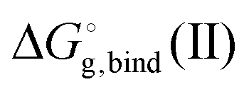
The solvation free energies within the cluster-continuum model are calculated using an appropriate thermodynamic cycle. The individual components of the thermodynamic cycle are evaluated separately. Bryantsev, Diallo and Goddard have discussed two distinct cycles that can be used within the cluster-continuum approach.⁴⁸ The monomer cycle (Fig. 1a) is identical to the approach introduced by Pliego and Riveros.³⁶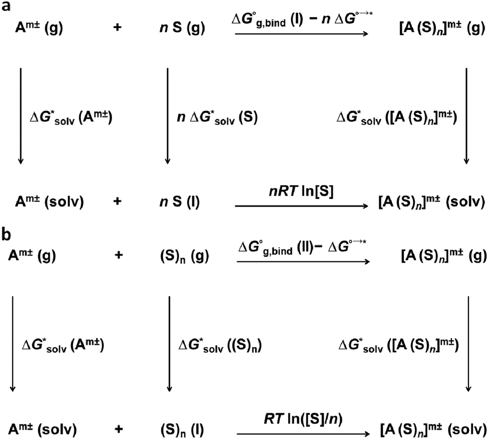

Fig. 1 (a) Monomer cycle used within the cluster-continuum model for the calculation of solvation free energies of ions. Solvent molecules are transferred from the liquid solvent into the gas phase. A cluster of the ion and n solvent molecules is formed in the gas phase. Then, the cluster is solvated within the dielectric-continuum model. Corrections arising from the 1 mol dm⁻³ standard state used for all components are added. (b) Cluster cycle used within the cluster-continuum model for the calculation of solvation free energies of ions. A cluster of n solvent molecules is taken from the liquid solvent to the gas phase. A cluster of the ion and n solvent molecules is formed in the gas phase. Subsequently, the cluster is solvated within the dielectric-continuum model. Corrections arising from the 1 mol dm⁻³ standard state used for all components are added.

Here, we use n individual solvent molecules to form a cluster with the ion in the gas phase and the formed cluster is then solvated using the implicit model. The cluster cycle (Fig. 1b) starts from the cluster of n solvent molecules reacting with the ion. The next step is identical to the monomer cycle, the cluster of the ion and solvent molecules is solvated implicitly.

We should pay special attention to the correct choice of the standard states in the calculations – all calculations must be performed with respect to the same standard state.

Experimental results are typically reported for a standard state of an infinitely diluted system extrapolated to the concentration of 1 mol dm⁻³. Electronic structure codes, on the other hand, provide data for a standard state of an ideal gas at 1 atm. The free-energy change of the transition of an ideal gas from 1 atm (24.46 dm³ mol⁻¹) to 1 mol dm⁻³ at T = 298.15 K is

ΔG°^→* = −TΔS°^→* = RT ln(V₀/V*) = RT ln(24.46) = 7.9 kJ mol⁻¹

This correction is used in the calculation of the free energy of cluster formation in both thermodynamic cycles. The correction is negative because the number of reactants is bigger than of the products. A detailed explanation of the corrections can be found in ref. 48.

A second correction is needed for the solvation of the solvent in the thermodynamic cycle. Let us assume water as an example. The concentrations of H₂O and (H₂O)_n in liquid water are 55.34 mol dm⁻³ and 55.34/n mol dm⁻³, respectively. The total change in the free energy for the reaction in the lower leg of the monomer cycle is zero in the case of 55.34 mol dm⁻³ water concentration. But 1 mol dm⁻³ standard state is required for all the entities. The correction is

nRT ln[H₂O]

if n water molecules are used within the monomer cycle. Similarly, the correction is

RT ln([H₂O]/n)

if the cluster of n water molecules is used within the cluster cycle.

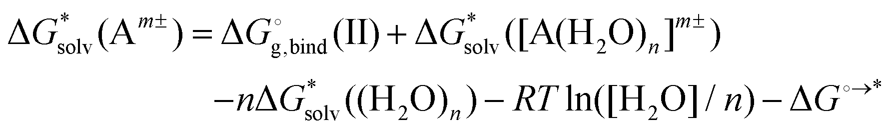
Adopting the monomer cycle and considering the corrections, the formula for the solvation free energy (A^m±) is given for water solvent as

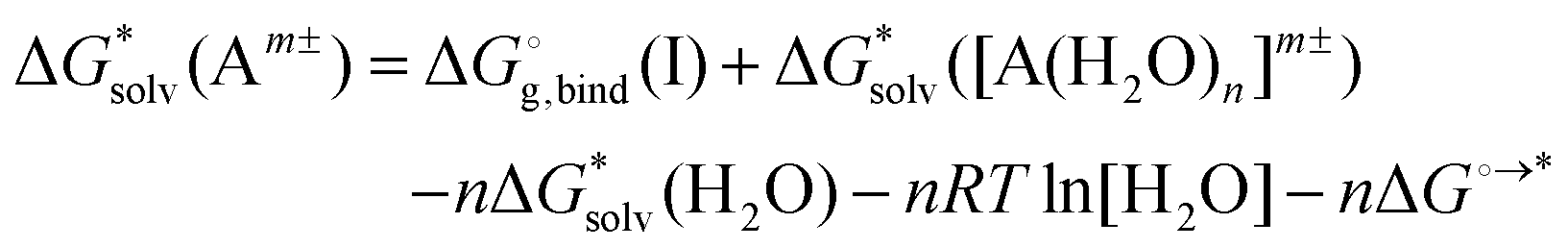
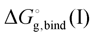where is the free energy of cluster formation from an ion and n separate molecules of solvent in the gas phase at 1 atm, ([A(H₂O)_n]^m±) is the solvation free energy of an ion–water cluster and (H₂O) is the solvation free energy of a single water molecule obtained using a desired implicit solvation model.

This approach was first systematically studied in 2001 on the set of 14 univalent ions using isodensity polarizable continuum model (IPCM)⁴⁹ as an implicit solvation model and the average error in the calculated solvation free energies was 36 kJ mol⁻¹.³⁶ However, the authors highlighted the lower standard deviations for the average error compared to the unaided dielectric models (in this work, we refer to the unaided calculations when no explicit solvent molecules were involved). Since then, various results have been published for the cluster-continuum model, some of them showed a very good agreement with experimental data.^48,50–52 Unfortunately, the general problem of the approach has not been solved; the approach relies on the global minimum of clusters which is difficult to find, especially for larger clusters.

Moreover, the method does not converge with the increasing number n of solvent molecules used within the monomer cycle. The convergence problem arises because separate water molecules are used in the cycle.⁴⁸ The systematic errors in the calculated solvation free energies are to some extent mitigated in the cluster cycle because hydrogen-bonded water clusters of the same size appear on both sides of the reaction. The solvation free energy of the ion according to the cluster cycle is given as

where is the free energy of the cluster formation from an ion and a water cluster consisting of n molecules in the gas phase at 1 atm, ([A(H₂O)_n]^m±) is the solvation free energy of an ion–water cluster and ((H₂O)_n) is the solvation free energy of a water cluster.

The cluster cycle provides results that converge with the number of solvent molecules in the cluster but for a high price. Again, the global minima for the clusters must be found. In addition, the authors⁴⁸ emphasized the importance of the correct choice of the number of water molecules used in the cluster cycle. They concluded that the best results could be obtained by using n = 6, 10, 14, 18…, for other numbers, their results deviated from the experiment.

1.2 Ensemble cluster-continuum approach for solvation free energies of ions

As we mentioned before, a large number of local minima, especially for larger clusters, complicates cluster-continuum calculations. The problem can be especially severe for large ions where even the first solvation shell contains many solvent molecules. The convergence of the cluster-continuum model is then difficult to assess.

We suggest an alternative thermodynamic cycle that does not require the optimization of clusters. Moreover, it contains charge neutralization steps in order to directly calculate only solvation free energies of neutral solutes because we assume that implicit models provide an accurate description of neutral systems. The model is called “Ensemble Cluster-Continuum” (EnCC) here and the respective thermodynamic cycle is presented in Fig. 2.

Fig. 2 Thermodynamic cycle (“EnCC cycle”) proposed for the calculation of solvation free energies of anions within EnCC. First, an anion is ionized in the gas phase. Then the neutral specie is solvated using a dielectric model. Finally, the solvated neutral is transformed into anion again.

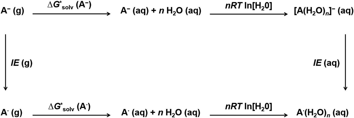
The solvation free energy is calculated in several steps. For clarity, we demonstrate the scheme on an example of a molecular anion. The geometry of the anion is kept fixed in its equilibrium geometry during all calculations. First, we calculate the ionization energy of the anion in the gas phase. This is a single calculation because the anion geometry is frozen. Second, we calculate the solvation free energy of the formed radical. This is again only a single calculation and we assume that the implicit model performs reasonably. Third, we calculate the adiabatic ionization energy of the anion in the liquid phase (or the electron affinity for the radical).

The latter quantity deserves a more detailed explanation. We calculate the ionization energy for an ensemble of clusters taken from the MD simulation. In our case, we prepared the ensemble via classical molecular dynamics simulation at finite temperature, using QM/MM model described in the Computational Details. The sampling method was selected pragmatically to avoid time-consuming ab initio MD or force field parametrization for solutes. The geometry of the anion is again kept fixed in its equilibrium geometry during the whole MD simulation.

The goal of the third step is to calculate adiabatic ionization energy (AIE). Here, we benefit from previous successful calculations of vertical quantities in the extended cluster-continuum model, such as vertical excitation energy or vertical ionization energy (VIE).^{45–47,53,54} In our approach, we let the outer sphere described by a dielectric continuum to fully relax. For the inner sphere, we calculate vertical quantities (〈VIE〉_DR, where the subscript DR denotes “full dielectric relaxation”) for the ensemble of structures sampling (classical) thermal equilibrium. We can extract the inner sphere reorganization energy λ using the well-known Marcus relation⁵⁵

where σ is the variance of the ionization energy distribution. The adiabatic ionization energy is then calculated

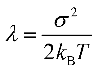
AIE = 〈VIE〉_DR − λ

Note that the transition from a species solvated in a dielectric continuum into the cluster embedded in the polarizable continuum is accompanied by a correction of nRT ln[S] (the solvent is water in our case) but these corrections cancel out so that the final formula reads(A⁻) = IE(g) + (A˙) − IE(aq) = IE(g) + (A˙) − 〈VIE〉_DR + λThe implementation of the above scheme has its limits. It will not be useful for situations where the solute structure changes significantly upon solvation. We also rely on the accurate estimation of the free energy of solvation for the neutral solute. Finally, the application of the Marcus formula assumes a linear response regime. Despite it, the scheme is a reasonable framework to study the convergence of the cluster-continuum approach.

2 Computational details

2.1 Cluster-continuum calculations

We performed solvation free energies calculations via the monomer and the cluster cycle using three different electronic structure approaches: Hartree–Fock (HF) method, hybrid B3LYP functional and long-range corrected functional LC-ωPBE.⁵⁶ We used 6-31+g* basis set in all calculations.

For the calculation of the solvation free energy using the monomer cycle, three components were evaluated. The free energy of cluster formation was calculated as

where n is the number of water molecules in a cluster and G°([A(H₂O)_n]^m±), G°(A^m±) and G°(H₂O) are free energies of an ion–water cluster, an ion and a water molecule, respectively. All geometries were optimized at the respective level of theory and the minimum was confirmed by the frequency calculation. The solvation free energy of the cluster, [A(H₂O)_n]^m±, was estimated using PCM and SMD models encompassing the standard procedure in the Gaussian code, where the gas-phase optimized structure was used in the calculation without any further optimization in SMD or PCM.⁵⁷ Default parameters used in our calculations are SMD atomic radii²⁵ with van der Waals surface cavity type with parameter α = 1.0 for SMD and universal force field (UFF) radii⁵⁸ with a scaled van der Waals cavity type with parameter α = 1.1. The same procedures were also used for the calculation of the solvation free energy, (H₂O), of the water molecule.

There are three components to evaluate in the cluster cycle. One of them, [A(H₂O)_n]^m±, is the same as in the monomer cycle. The solvation free energy ((H₂O)_n) was calculated for the gas-phase optimized water clusters; starting geometries for the optimization were taken from ref. 59. The energy of the cluster formation was obtained as

where the only alteration from the case of the monomer cycle is that the free energy of one water cluster consisting of n molecules was used.

All the calculations were performed in the Gaussian 09 (revision D.01) suite of codes.⁶⁰

2.2 Ensemble cluster-continuum approach

For all calculations involving ions as well as radicals within EnCC, the same frozen structure of ions was used. This structure was obtained by optimizing the ion in the gas phase at the B3LYP/6-31+g* level.

The molecular dynamics of the ion surrounded by water molecules was performed by our in-house code ABIN⁶¹ interfaced to GPU based Terachem v 1.93 software.^62,63 The optimized ion structure was fixed during the dynamics simulation. The ions were always solvated in a droplet of 500 water molecules. The initial arrangement of the water molecules was created by Packmol software.⁶⁴ The simulation was performed at the QM/MM level using the B3LYP/6-31+g* functional with Grimme's dispersion correction D2.⁶⁵ The QM part involved only the ion, the MM part was described by the TIP3P model.^66,67 The temperature was kept at 298.15 K during the simulation by Nosé–Hoover thermostat. The time step of 0.5 fs was used with a total of 50 000 steps (25 ps). Only geometries from the last 15 ps were used for the subsequent calculations of the ionization energy in liquid. It was used 1500 geometries in total with the equidistant step of 10 fs. The number of configurations could be in fact reduced, considering the correlation between the samples. For a case of Ca²⁺ ion we also performed a classical simulation of one molecule of CaCl₂ in a 99.8 Å box of water, the force field parameters were taken from ref. 68. The simulation step was 2 fs, the temperature of 300 K was controlled by the v-rescale thermostat with coupling time 0.1 ps, the pressure of 1 bar was controlled by the Parrinello–Rahman barostat with coupling time of 2 ps. The total length of simulation was 80 ns from which we selected equally distances 50 frames and from these 50 frames we started the 5 ps MD as stated above to avoid the correlection of structures. Only the last frame (after 5 ps) was taken from each of 50 simulations.

The three types of calculations of the EnCC approach were performed again at HF/6-31+g*, B3LYP/6-31+g* and LC-ωPBE/6-31+g* levels. The solvation free energy of neutral species, (A˙), is calculated with the PCM or SMD methods with the parametrization implemented in the Gaussian 09 code for the fixed geometry of the ion. The gas-phase ionization energy, IE(g), was calculated using the difference in the electronic energies of the ion and the radical, again for the same fixed geometry of the ion. For the calculation of the ionization energy in liquid, IE(aq), 1500 structures from molecular dynamics were used. Those structures contained only the ion and the n closest water molecules (with n ranging from 1 to 20) and kept fixed during the ionization calculations. The PCM and SMD models with default parameters were used for the calculations as implemented in the Gaussian 09 code.

Aside from the EnCC, we also calculated vertical ionization energies for the same set of structures from molecular dynamics (number of explicit water molecules was 0, 1, 5 and 10) to assess the accuracy of the electronic structure methods. The values were obtained using non-equilibrium PCM or non-equilibrium SMD as implemented in the Gaussian 09 code. The average from 1500 sampled geometries was assumed in all the calculations.

The calculations were performed for a set of ions containing Cl⁻, CH₃O⁻, SCN⁻, S²⁻, Na⁺, Ca²⁺ and Li⁺. The set was selected in order to include various ion types – monoatomic and polyatomic systems, anions and cations, singly and multiply charged systems.

3 Results and discussion

3.1 Chloride anion: detailed study

We started the investigation of the EnCC approach on an example of an atomic chloride anion. It was selected because it is a simple atomic ion and a full range of data needed for the critical evaluation of the method is available. A direct comparison of the calculations with the experiment can be done for the total solvation free energy as well as for all the partial energies used in the EnCC thermodynamic cycle.

Fig. 3 shows the calculated solvation free energies within the EnCC model. We compare three different electronic structure methods (HF, LC-ωPBE, and B3LYP) and two different dielectric continuum models (PCM and SMD), where the difference is chiefly due to the different radii of the molecules. We observe that the values calculated only with the dielectric continuum models are off the experimental range. The addition of explicit water molecules improves the agreement with the experimental values. The solvation free energy obtained with different methods tends to approach the “real” value with the SMD solvation model while it is close to the “bulk” value for the PCM model. It is consistent with the SMD parametrization for the “real” scale.²⁵ It is interesting to notice that the difference between these two models does not decrease with the increasing number of solvating molecules. This necessarily stems from the different descriptions of the QM/continuum interface. The two dielectric models should provide identical results for the infinite size of the clusters, yet we are far from this limit with several tens of solvating water molecules. We also examined how the solvation free energies converge with increasing the basis set size. As we demonstrate in Table S4 in ESI,† there is only a minor effect.

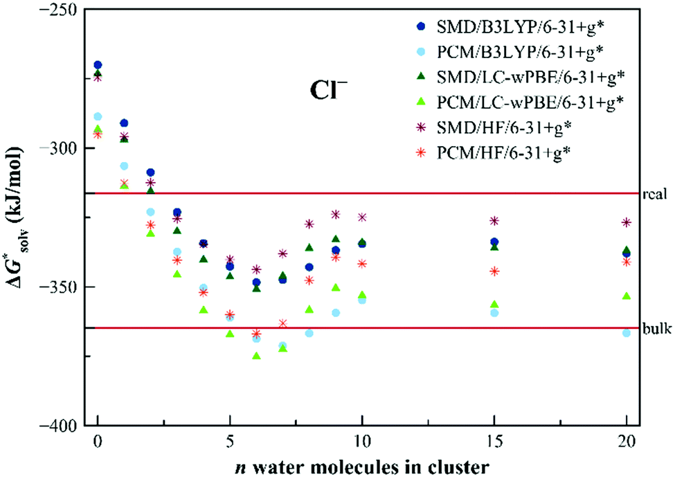Fig. 3 Calculated solvation free energies (kJ mol⁻¹) of Cl⁻ from EnCC cycle using different electronic structure methods and different numbers of explicit water molecules. Experimental value denoted as “bulk” is taken from ref. 3 and is then recalculated to the “real” scale using Tissandier's value of the hydration free energy of the proton.⁶

The EnCC approach also provides a natural possibility to evaluate error bars of calculated values since the calculations are performed on an ensemble of structures. The results together with error bars can be found in ESI† (Fig. S3–S5). It is seen that increasing the cluster size mitigates the systematic error at a price of an increased statistical error.

We also calculated the solvation free energy of Cl⁻ using the canonical versions of the cluster-continuum model. The performance of the monomer cycle, as well as the cluster cycle, was examined and results are summarized in Table 1. The monomer cycle, as originally derived by Pliego and Riveros,³⁶ provides values of solvation free energies that raise from one to three explicit water molecules involved in the calculation. The result closest to the experimental value (−316 kJ mol⁻¹, “real” value) was achieved with the PCM/LC-ωPBE/6-31+g* using one explicit water molecule. The results for the cluster cycle, as described in ref. 48, were calculated as well. The cluster approach seems to improve the accuracy of the results from clusters containing more than one water molecule. It agrees well with the claim of authors in ref. 48 that the errors are mitigated to some extent when using the hydrogen-bonded clusters of the same size on both sides of the reaction. Still, the best agreement with the experimental value is achieved by using just one water molecule. However, to reliably explore the results from the cluster cycle, one would have to add more explicit water molecules which would also require the minima search. Finding those minima of large clusters is, however, not of primary interest in our study. Nevertheless, the cluster cycle approach for the calculation of the solvation free energy of a chloride anion was performed in the study of Riccardi et al.⁵¹ They used MP2 level with the estimated complete basis set limit and different dielectric models. When the clusters with 8 water molecules were used, they reached the values of −305 and −309 kJ mol⁻¹ for SMD with default SMD radii and PCM with Bondi radii, respectively. However, the values they obtained for the lower numbers of water molecules varied the same way as our results in Table 1.

Table 1 Calculated solvation free energies (kJ mol⁻¹) of Cl⁻ using cluster-continuum model with the monomer cycle and the cluster cycle and different electronic structure methods

Method	Monomer cycle			Cluster cycle
	Number of explicit waters in cluster
	1	2	3	1	2	3
a Experimental value is taken from ref. 3 and it is then recalculated to the “real” scale using Tissandier's hydration free energy of the proton.^6
PCM/B3LYP/6-31+g*	−295	−286	−268	−295	−286	−279
SMD/B3LYP/6-31+g*	−276	−262	−235	−276	−268	−267
PCM/LC-ωPBE/6-31+g*	−298	−289	−271	−298	−289	−283
SMD/LC-ωPBE/6-31+g*	−278	−263	−236	−278	−270	−269
PCM/HF/6-31+g*	−294	−278	−255	−294	−278	−272
SMD/HF/6-31+g*	−273	−253	−222	−273	−260	−258
Experimental value	−316^a

---

We also explored partial energetic data in the EnCC thermodynamic cycle, using the following experimental data. The adiabatic ionization energy of the chloride anion in the aqueous phase was calculated from the redox potentials

Cl˙ + e⁻ → Cl⁻ 2.43 V (rel.⁶⁹)

2H⁺ + 2e⁻ → H₂ 4.28 V (abs.^70,71)

The resulting value is 6.71 V (647 kJ mol⁻¹) for the adiabatic ionization energy of the chloride anion in the aqueous phase. Note that this value depends on the choice of the absolute electrode potential of the hydrogen electrode and it is therefore related to the proton solvation free energy associated with some experimental uncertainty. The selected value of 4.28 V is thermodynamically consistent with the absolute solvation free energy of the proton of −1113 kJ mol⁻¹ derived by Tissandirer.⁶ The solvation free energy of the Cl radical can be calculated via a simple thermodynamic cycle using the solvation free energy of Cl⁻ and ionization energies in the gas phase (taken directly from ref. 72) and aqueous phase(Cl˙) = −IE(g) + (Cl⁻) + IE(aq) = (−349 − 316 + 647) kJ mol⁻¹ = −18 kJ mol⁻¹

The comparison of the experimental data with our calculations is shown in Table 2. We first focus on the ionization energy in the gas phase, IE(g). We see that range-separated functional LC-ωPBE provides the gas-phase ionization energy in an excellent agreement with the experimental value. On the other hand, the HF method yields a value largely deviating from the experiment. The situation is analogical for the ionization energies in the aqueous phase. The HF method predicts much lower IE compared with the experiment, the error associated with the electronic structure theory, however, largely cancels out in the EnCC thermodynamic cycle and the solvation free energy can be reliable.

Table 2 Evaluated components (kJ mol⁻¹) of the solvation free energy of Cl⁻ using the EnCC approach described by the EnCC thermodynamic cycle. Results from different calculation methods are presented

Method	IE(g)	(Cl˙)	IE(aq), number of explicit waters
			0	1	5	10	20
a Ref. 72. b Calculated from experimental values of the ionization energy in the gas phase,^72 the ionization energy in the aqueous phase^69–71 and the solvation free energy.^3,6 c Calculated from redox potential^69 using the absolute electrode potential of the hydrogen electrode.^70,71
PCM/B3LYP/6-31+g*	358	−2.9	644	662	716	710	722
SMD/B3LYP/6-31+g*	358	0.4	629	650	701	693	697
PCM/LC-ωPBE/6-31+g*	350	−2.9	640	661	714	700	700
SMD/LC-ωPBE/6-31+g*	350	0.4	623	647	697	685	687
PCM/HF/6-31+g*	239	−3.3	531	548	595	577	577
SMD/HF/6-31+g*	239	0.4	514	535	579	564	566
Experimental value	349^a	−18^b	647^c

---

We can further look at the changes associated with the addition of explicit water molecules. The general feature is an increase in IE(aq) with the number of explicit water molecules, clearly visible for a small number of solvating molecules. Further, an increase in the number of solvating molecules does not change the calculated adiabatic ionization energy significantly (see Fig. S1 in ESI†). The calculated data are somewhat higher than the experimental ones; note, however, that the experimental data are derived for a particular value of the absolute electrode potential of the hydrogen electrode.

The solvation free energy of the neutral species seems to be described reasonably well with both the SMD and PCM methods when considering the uncertainties of used experimental data. The results do not depend on the electronic structure method used, it is rather controlled by the construction of the cavity used in the polarizable continuum model.

Further insight into the quality of the calculated data can be gained from the inspection of the first vertical ionization energy. This quantity does not enter directly the calculation of solvation free energy yet can indicate potential problems of the respective methods. Further, the experimental data are independent of the assumed proton solvation energy value. The results are summarized in Table 3. Again, the HF method does not provide quantitatively accurate results because of the lack of correlation energy. The best agreement with the experiment is achieved with the range-separated functional LC-ωPBE. The B3LYP functional provides results different by almost 85 kJ mol⁻¹ from the experiment. This discrepancy is mostly associated with the self-interaction error, manifested by artificial spin delocalization in the neutral system. Note, however, that the difference between the LC-ωPBE and the B3LYP methods is much smaller for the adiabatic ionization energy compared to the vertical ionization energy.

Table 3 Calculated vertical ionization energies (kJ mol⁻¹) of Cl⁻ using different electronic structure methods as a function of the number of explicit water molecules

Method	Number of explicit waters
	0	1	5	10
a Ref. 73.
PCM/B3LYP/6-31+g*	812	820	858	854
SMD/B3LYP/6-31+g*	782	799	849	845
PCM/LC-ωPBE/6-31+g*	812	828	900	925
SMD/LC-ωPBE/6-31+g*	782	803	879	895
PCM/HF/6-31+g*	703	720	782	808
SMD/HF/6-31+g*	669	695	761	778
Experiment	925^a

---

To summarize, the LC-ωPBE method describes correctly the energetics of all three components in the EnCC cycle and the value of solvation free energy is reliable. The HF method does not describe quantitatively the energetics of the ionization consistently both in the gas phase and in the liquid phase due to the lack of electron correlation, yet these contributions cancel out. The B3LYP functional suffers from the problem of self-interaction error which does not cancel out in the EnCC cycle and its use is problematic.

3.2 Solvation free energies for other ions

The EnCC approach was also tested for other ions, namely CH₃O⁻, SCN⁻, S²⁻, Na⁺, Ca²⁺ and Li⁺. For these ions, also the canonical cluster-continuum values (via the monomer cycle) were calculated, the results are presented in Table 4. The calculated values are closer to the experimental values for the PCM model, compared to SMD, for SCN⁻, S²⁻, and Na⁺. On the other hand, cluster-continuum models provide results much closer to the experiment for CH₃O⁻ and Ca²⁺ with the SMD model. The canonical cluster-continuum approach fails for the doubly-charged ions as well as for the CH₃O⁻ ion irrespective of the model used. In these cases, the ions have high charge density and a larger number of solvating molecules is needed. Next, we applied the EnCC approach. First, the values of (A˙) were evaluated. Comparison of the performance of SMD, PCM and canonical cluster-continuum for neutrals can be found in ESI† (Tables S1 and S2) and indicates that dielectric models perform reasonably well for neutral species.

Table 4 Calculated solvation free energies (kJ mol⁻¹) for different ions using cluster-continuum model with the monomer cycle and HF method with PCM or SMD solvation model

Ion/method	Number of explicit waters in cluster			Experiment
	1	2	3
For SCN^−, S^2−, Na^+, and Ca^2+ the experimental values were taken from the work of Marcus^3 which were then recalculated to the “real” scale using Tissandier's hydration free energy of proton; for CH3O^−, the “real” value was taken from ref. 38. Thus, all the experimental data in the table refer to the “real” scale.
CH3O^−/SMD	−351	−338	−320
CH3O^−/PCM	−328	−332	−331	−398
SCN^−/SMD	−215	−200	−164
SCN^−/PCM	−234	−226	−199	−246
S^2−/SMD	−992	−977	−957
S^2−/PCM	−1051	−1038	−1021	−1283
Na^+/SMD	−337	−366	−380
Na^+/PCM	−422	−425	−420	−432
Ca^2+/SMD	−1606	−1596	−1577
Ca^2+/PCM	−1473	−1477	−1474	−1616
Li^+/SMD	−426	−466	−485
Li^+/PCM	−511	−512	−508	−538

---

The convergence of solvation free energies calculated with the EnCC approach for CH₃O⁻ is demonstrated in Fig. 4. Both dielectric models fail to reproduce the experimental values of the solvation free energy, irrespective of the proton solvation free energy convention. This disagreement is caused by the high concentration of the negative charge on the oxygen atom. Our calculations demonstrate a visible shift of the calculated solvation free energies with the increasing number of solvating water molecules. The results tend to converge to the values close to the experimental ones, especially when using the SMD method.

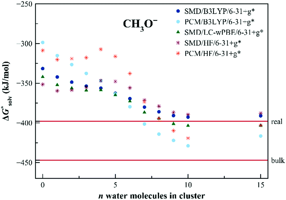Fig. 4 Calculated solvation free energies (kJ mol⁻¹) of CH₃O⁻ from the EnCC cycle using different electronic structure methods and different numbers of explicit water molecules. Experimental value denoted as “real” is taken from ref. 38 and is then recalculated to the “bulk” scale using Marcus hydration free energy of the proton.³

The calculated solvation free energies for the SCN⁻ anion are shown in Fig. 5. The solvation free energies are reasonably well described already within the dielectric models without any additional water molecules. The charge is more distributed over the solute in this case. We still observe, however, a shift upon the addition of the explicit water molecules, converging to the values in between the “real” and “bulk” ones. As for the Cl⁻ anion, the PCM model seems to provide results closer to the “bulk” scale.

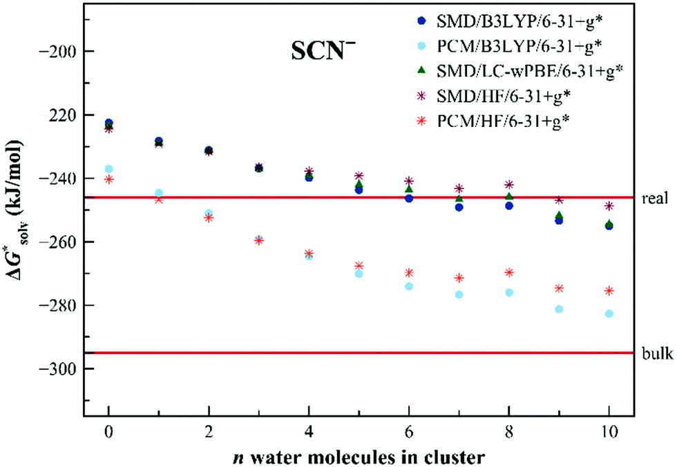Fig. 5 Calculated solvation free energies (kJ mol⁻¹) of SCN⁻ from the EnCC cycle using different electronic structure methods and different numbers of explicit water molecules. Experimental value denoted as “bulk” is taken from ref. 3 and is then recalculated to the “real” scale using the Tissandier hydration free energy of the proton.⁶

Calculating solvation free energies of doubly-charged ions is a challenging task for the dielectric continuum models. The convergence can be extremely slow as has been demonstrated earlier.⁷⁴ The error of the calculated solvation free energy for the S²⁻ anion is as large as 200 kJ mol⁻¹ for the dielectric models and the situation does not improve upon the addition of a small number of solvating molecules. Fig. 6 shows the results obtained with the EnCC model. The convergence is slow but we observe a similar trend with an increasing number of water molecules as for Cl⁻. We observe a drop in solvation free energy at around n = 10, followed by a further rise for n = 15.

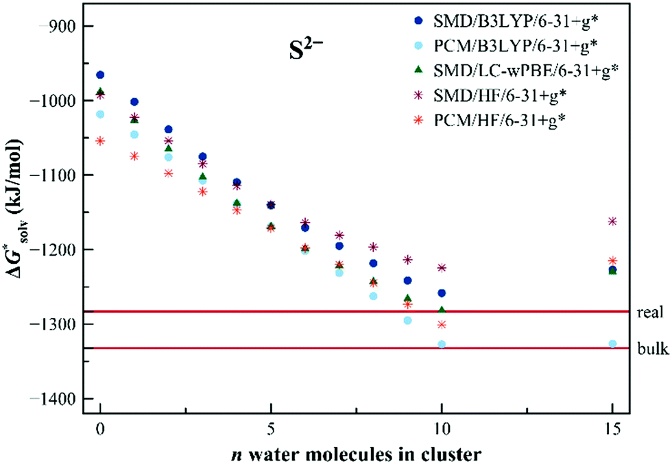Fig. 6 Calculated solvation free energies (kJ mol⁻¹) of S²⁻ from the EnCC cycle using different electronic structure methods and different numbers of explicit water molecules. Experimental value denoted as “bulk” is taken from ref. 3 and is then recalculated to the “real” scale using the Tissandier hydration free energy of the proton.⁶

We assume that the convergence curve is analogous to the chloride anion, i.e. we can expect a slight decrease for n larger than 15. As before, the calculated quantities differ between SMD and PCM, yet the differences between the two models are much smaller than the variations within the number of explicit solvent models included in the simulations.

The results of the EnCC based solvation free energies for Na⁺ are shown in Fig. 7. The unaided SMD model provides solvation energy higher than the experimental value by more than 100 kJ mol⁻¹, the unaided PCM model provides results within the experimental range. It is interesting that, unlike in previous cases, the HF and LC-ωPBE methods provide the same results for the bigger clusters irrespective of the dielectric model. Results from the B3LYP method differ from the two others. This is probably a general problem of the density functional theory, related to the size-dependent delocalization ionization potential error.^75,76 The electron artificially delocalizes in the extended systems and the ionization then takes place from the solvent molecules as well as from the solute. The situation can be remedied with the use of the range-separated functional with a higher value of range separation parameter,⁷⁵ as is the LC-ωPBE functional used in this work. The results from the HF or range-separated methods are therefore more reliable. The residual discrepancy between the performance of the EnCC method (with HF or LC-ωPBE) and the experimental value can be explained as insufficiency in the description of neutral Na via the unaided SMD solvation model.

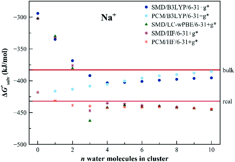Fig. 7 Calculated solvation free energies (kJ mol⁻¹) of Na⁺ from the EnCC cycle using different electronic structure methods and different numbers of explicit water molecules. Experimental value denoted as “bulk” is taken from ref. 3 and is then recalculated to the “real” scale using the Tissandier hydration free energy of the proton.⁶

The results for Ca²⁺ are shown in Fig. 8. Even the dielectric models provide a reasonable description of the solvation. The results for Ca²⁺ are shown in Fig. 8. Even the dielectric models provide a reasonable description of the solvation energetics – which indicates a suitable choice of the ionic radius for the cation. There is no strong evolution of the calculated solvation free energy with the cluster size. The B3LYP data seem to over-perform the other two methods yet the differences are relatively small.

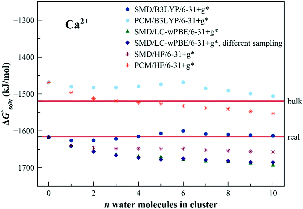Fig. 8 Calculated solvation free energies (kJ mol⁻¹) of Ca²⁺ from the EnCC cycle using different electronic structure methods and different numbers of explicit water molecules. Data denoted as “different sampling” are obtained using a different ensemble of frames as described in Computational details. Experimental value denoted as “bulk” is taken from ref. 3 and is then recalculated to the “real” scale using the Tissandier hydration free energy of the proton.⁶

We would like to point out, that the employed MD sampling method is not a particularly good choice for Ca²⁺ because the length of ab initio MD is not appropriate for sampling all relevant hydration sites. We, therefore, calculated the single ion solvation free energy for a case when the sampling was performed differently (by a series of short QM/MM simulations starting from a preliminary classical simulation, see the Computational details). Surprisingly, the results for both approaches are similar. This fact indicates that reliable results could be obtained even by using much smaller ensembles of clusters, assuming that the individual frames are uncorrelated.

The calculated solvation free energies for Li⁺ ion are shown in Fig. 9. Unaided SMD fails to predict the solvation free energy by more than 130 kJ mol⁻¹, whereas unaided PCM provides results in the experimental area. With the increasing number of explicit water molecules, SMD-based calculations provide results that rapidly drop to the experimental area. Similarly to Na⁺, HF and LC-ωPBE results are close irrespective of the dielectric model used. In this case, the results can be directly compared with the approach by Duignan et al.²² discussed in the Introduction. Our result obtained with the LC-ωPBE functional together with the SMD dielectric model shows very good agreement with Duignan's data.

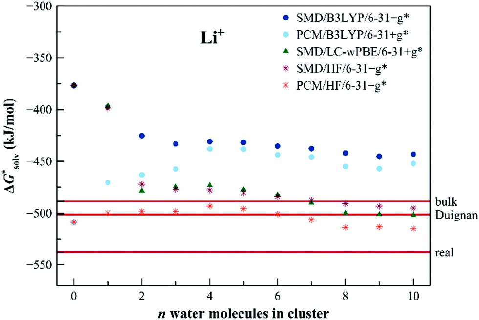Fig. 9 Calculated solvation free energies (kJ mol⁻¹) of Li⁺ from the EnCC cycle using different electronic structure methods and different numbers of explicit water molecules. Experimental value denoted as “bulk” is taken from ref. 3 and is then recalculated to the “real” scale using the Tissandier hydration free energy of the proton.⁶ “Duignan” refers to the result obtained by Duignan et al.²²

4 Conclusions

In the present work, we proposed an alternative scheme for the cluster-continuum calculation of solvation free energies. The scheme is based on a thermodynamic cycle, involving ionization in the gas phase and the liquid state. The latter quantity can be evaluated for an ensemble of structures sampled by classical molecular dynamics. We, therefore, refer to this approach as to Ensemble Cluster-Continuum (EnCC) model.

We have shown that the present approach asymptotically provides values of the hydration free energies that fit within the experimental error bounds. The approach works well especially for anions, including multiply charged anions with a high charge density. The approach seems to outperform the usual cluster-continuum techniques in some respect and can represent a practical way for the theoretical evaluation of solvation free energies. Note, however, that the utility is limited by the computational cost of the approach – some quantities have to be evaluated for an ensemble of structures. We should also point out that the sampling procedure should be carried out carefully. Systems with the water exchange rate on the scale of hundreds of picoseconds or longer require much longer MD simulations or a combination of classical MD simulations and ab initio ones.^77,78

The EnCC approach is from our perspective important because it can provide a measure of systematic error of the dielectric continuum model. Performing the systematic investigation of the solvation free energy convergence, we can set the degree of reliability for the quantity calculated with the dielectric continuum model itself. Quantum chemical calculations typically provide values with an accuracy based solely on the experience. The systematic cluster-continuum approach is one of the ways to circumvent the limitation.

The present approach has certain limitations. First, typically only small clusters are treated. The numerical value of the calculated quantities will still critically depend on the dielectric continuum model used. Second, the typically used electronic structure approaches can be accurate for isolated molecules, yet they can have a poor performance for solvated molecules in clusters. This is especially the case of the DFT methods, with well-know (yet often underestimated) problems connected to the self-interaction error. In the present case, some problems can be magnified because open-shell systems are modelled in certain steps of the calculations. Range-separated functional represent, however, a robust choice. Third, the method is based on the assumption that the solvation free energy of the neutral species can be reliably estimated within the dielectric continuum models. This is often the case (especially for the anions), yet there are exceptions. Next, the presented method can not be directly used to anions whose ionization energy is higher than of water (e.g. F⁻) and in these cases, the calculations on the ensemble of structures need to be conducted differently, for example using Koopmans’ theorem,⁷⁹ the Maximum Overlap Method (MOM),⁸⁰ ionization as excitation method or QM:QM approach.¹¹ Finally, we need to sample the cluster structures. This can typically not be done at the same level of theory we use for the energy calculations which leads to further inconsistencies (see Fig. S2 in ESI†).

We conclude that the solvation free energies can hardly be estimated within the cluster-continuum approaches better than the experimental uncertainty given by the disputed proton solvation free energy. With the present method, the solvation free energies can be calculated within 40 kJ mol⁻¹. We envision the potential of the method especially for the highly unstable and multiply charged species. Such species can appear e.g. in the field of radiation chemistry where theory is often the easiest way to estimate the energetics.

As a general observation, we conclude that the proposed model for solvation free energies performs better when applied to anions. This is because of the charge neutralization which is at the core of our approach. In the case of anions, the charge neutralization leads to a loss of electrons which facilitates calculations in solution. In the case of cations, more electrons are added to the system via the charge neutralization and this could, on the contrary, complicate calculations in the solution.

The present approach to solvation follows the experimental way which can be achieved within the liquid jet model. Recent photoemission experiments provide us with high-resolution photoemission data, allowing in principle for a direct determination of the adiabatic ionization energy for a given half-reaction. Together with gas-phase data, this would allow for a direct determination of the absolute solvation free energy of the ions.

Conflicts of interest

There are no conflicts to declare.

Acknowledgements

The support by the Grant Agency of the Czech Republic, project no. 18-23756S is gratefully acknowledged. Part of the calculations was done on the IT4I, project number OPEN-18-51. The research leading to these results was supported by the European Structural and Investment Funds, OP RDE-funded project ‘CHEMFELLS III’ (CZ.02.269/0.0/0.0/19_074/0014006) funding MSCA-IF proposal.

References

1. C. P. Kelly, C. J. Cramer and D. G. Truhlar, J. Phys. Chem. B, 2006, 110, 16066–16081.
2. B. E. Conway, J. Solution Chem., 1978, 7, 721–770.
3. Y. Marcus, Ion Properties, CRC Press, New York, 1997.
4. P. Hunenberger and M. Reif, Single-Ion Solvation: Experimental and Theoretical Approaches to Elusive Thermodynamic Quantities, RSC Publishing, Cambridge UK, 2011.
5. Y. Marcus, J. Chem. Soc., Faraday Trans., 1991, 87, 2995–2999.
6. M. D. Tissandier, K. A. Cowen, W. Y. Feng, E. Gundlach, M. H. Cohen, A. D. Earhart and J. V. Coe, J. Phys. Chem. A, 1998, 102, 7787–7794.
7. C. C. Doyle, Y. Shi and T. L. Beck, J. Phys. Chem. B, 2019, 123, 3348–3358.
8. T. P. Pollard and T. L. Beck, J. Chem. Phys., 2018, 148, 222830.
9. N. F. Carvalho and J. R. Pliego, Phys. Chem. Chem. Phys., 2015, 17, 26745–26755.
10. A. Warshel and M. Levitt, J. Mol. Biol., 1976, 103, 227–249.
11. Z. Tóth, J. Kubečka, E. Muchová and P. Slavíček, Phys. Chem. Chem. Phys., 2020, 22, 10550–10560.
12. R. M. Richard, K. U. Lao and J. M. Herbert, J. Chem. Phys., 2014, 141, 014108.
13. K. U. Lao, K.-Y. Liu, R. M. Richard and J. M. Herbert, J. Chem. Phys., 2016, 144, 164105.
14. C. Ochsenfeld, J. Kussmann and D. S. Lambrecht, Rev. Comput. Chem., 2007, 1–82.
15. S. B. Rempe, L. R. Pratt, G. Hummer, J. D. Kress, R. L. Martin and A. Redondo, J. Am. Chem. Soc., 2000, 122, 966–967.
16. D. Asthagiri, L. R. Pratt and H. S. Ashbaugh, J. Chem. Phys., 2003, 119, 2702–2708.
17. A. Grossfield, P. Ren and J. W. Ponder, J. Am. Chem. Soc., 2003, 125, 15671–15682.
18. G. Lamoureux and B. Roux, J. Phys. Chem. B, 2006, 110, 3308–3322.
19. B. Lev, B. Roux and S. Y. Noskov, J. Chem. Theory Comput., 2013, 9, 4165–4175.
20. T. S. Hofer and P. H. Hünenberger, J. Chem. Phys., 2018, 148, 222814.
21. N. Prasetyo, P. H. Hünenberger and T. S. Hofer, J. Chem. Theory Comput., 2018, 14, 6443–6459.
22. T. T. Duignan, M. D. Baer, G. K. Schenter and C. J. Mundy, Chem. Sci., 2017, 8, 6131–6140.
23. B. Mennucci and J. Tomasi, J. Chem. Phys., 1997, 106, 5151.
24. E. Cancès, B. Mennucci and J. Tomasi, J. Chem. Phys., 1997, 107, 3032.
25. A. V. Marenich, C. J. Cramer and D. G. Truhlar, J. Phys. Chem. B, 2009, 113, 6378–6396.
26. A. Klamt and G. Schüürmann, J. Chem. Soc., Perkin Trans. 2, 1993, 799–805.
27. A. Klamt, J. Phys. Chem., 1995, 99, 2224–2235.
28. K. N. Marsh, J. Chem. Eng. Data, 2006, 51, 1480.
29. A. Klamt, B. Mennucci, J. Tomasi, V. Barone, C. Curutchet, M. Orozco and F. J. Luque, Acc. Chem. Res., 2009, 42, 489–492.
30. S. Mirzaei, M. V. Ivanov and Q. K. Timerghazin, J. Phys. Chem. A, 2019, 123, 9498–9504.
31. V. Barone, M. Cossi and J. Tomasi, J. Chem. Phys., 1997, 107, 3210–3221.
32. D. M. Chipman, J. Chem. Phys., 1997, 106, 10194–10206.
33. D. M. Chipman, J. Chem. Phys., 2000, 112, 5558–5565.
34. M. Cossi, N. Rega, G. Scalmani and V. Barone, J. Chem. Phys., 2001, 114, 5691–5701.
35. E. Cancès and B. Mennucci, J. Chem. Phys., 2001, 114, 4744–4745.
36. J. R. Pliego and J. M. Riveros, J. Phys. Chem. A, 2001, 105, 7241–7247.
37. C. P. Kelly, C. J. Cramer and D. G. Truhlar, J. Phys. Chem. A, 2006, 110, 2493–2499.
38. J. R. Pliego Jr and J. M. Riveros, Phys. Chem. Chem. Phys., 2002, 4, 1622–1627.
39. B. Thapa and H. B. Schlegel, J. Phys. Chem. A, 2015, 119, 5134–5144.
40. F. Arrigoni, R. Breglia, L. D. Gioia, M. Bruschi and P. Fantucci, J. Phys. Chem. A, 2019, 123, 6948–6957.
41. J. Li, C. L. Fisher, J. L. Chen, D. Bashford and L. Noodleman, Inorg. Chem., 1996, 35, 4694–4702.
42. G. M. Ullmann, L. Noodleman and D. A. Case, J. Biol. Inorg. Chem., 2002, 7, 632–639.
43. M. Uudsemaa and T. Tamm, J. Phys. Chem. A, 2003, 107, 9997–10003.
44. J. Pratuangdejkul, W. Nosoongnoen, G. A. Guerin, S. Loric, M. Conti, J. M. Launay and P. Manivet, Chem. Phys. Lett., 2006, 420, 538–544.
45. D. Yepes, R. Seidel, B. Winter, J. Blumberger and P. Jaque, J. Phys. Chem. B, 2014, 118, 6850–6863.
46. P. Jaque, A. V. Marenich, C. J. Cramer and D. G. Truhlar, J. Phys. Chem. C, 2007, 111, 5783–5799.
47. M. Rubešová, V. Jurásková and P. Slavíček, J. Comput. Chem., 2017, 38, 427–437.
48. V. S. Bryantsev, M. S. Diallo and W. A. Goddard, J. Phys. Chem. B, 2008, 112, 9709–9719.
49. J. B. Foresman, T. A. Keith, K. B. Wiberg, J. Snoonian and M. J. Frisch, J. Phys. Chem., 1996, 100, 16098–16104.
50. C.-G. Zhan and D. A. Dixon, J. Phys. Chem. A, 2004, 108, 2020–2029.
51. D. Riccardi, H.-B. Guo, J. M. Parks, B. Gu, L. Liang and J. C. Smith, J. Chem. Theory Comput., 2013, 9, 555–569.
52. A. Muralidharan, L. R. Pratt, M. I. Chaudhari and S. B. Rempe, J. Phys. Chem. A, 2018, 122, 9806–9812.
53. Y. Zhao and Z. Cao, J. Theor. Comput. Chem., 2013, 12, 1341013.
54. H. B. Guo, F. He, B. H. Gu, L. Y. Liang and J. C. Smith, J. Phys. Chem. A, 2012, 116, 11870–11879.
55. R. A. Marcus, J. Chem. Phys., 1956, 24, 966–978.
56. O. A. Vydrov and G. E. Scuseria, J. Chem. Phys., 2006, 125, 234109.
57. J. Ho, A. Klamt and M. L. Coote, J. Phys. Chem. A, 2010, 114, 13442–13444.
58. A. K. Rappe, C. J. Casewit, K. S. Colwell, W. A. Goddard and W. M. Skiff, J. Am. Chem. Soc., 1992, 114, 10024–10035.
59. T. James, D. J. Wales and J. Hernández-Rojas, Chem. Phys. Lett., 2005, 415, 302–307.
60. M. J. Frisch, G. W. Trucks, H. B. Schlegel, G. E. Scuseria, M. A. Robb, J. R. Cheeseman, G. Scalmani, V. Barone, B. Mennucci, G. A. Petersson, H. Nakatsuji, M. Caricato, X. Li, H. P. Hratchian, A. F. Izmaylov, J. Bloino, G. Zheng, J. L. Sonnenberg, M. Hada, M. Ehara, K. Toyota, R. Fukuda, J. Hasegawa, M. Ishida, T. Nakajima, Y. Honda, O. Kitao, H. Nakai, T. Vreven, J. J. A. Montgomery, J. E. Peralta, F. Ogliaro, M. Bearpark, J. J. Heyd, E. Brothers, K. N. Kudin, V. N. Staroverov, T. Keith, R. Kobayashi, J. Normand, K. Raghavachari, A. Rendell, J. C. Burant, S. S. Iyengar, J. Tomasi, M. Cossi, N. Rega, J. M. Millam, M. Klene, J. E. Knox, J. B. Cross, V. Bakken, C. Adamo, J. Jaramillo, R. Gomperts, R. E. Stratmann, O. Yazyev, A. J. Austin, R. Cammi, C. Pomelli, J. W. Ochterski, R. L. Martin, K. Morokuma, V. G. Zakrzewski, G. A. Voth, P. Salvador, J. J. Dannenberg, S. Dapprich, A. D. Daniels, O. Farkas, J. B. Foresman, J. V. Ortiz, J. Cioslowski and D. J. Fox, Gaussian 09, Revision D.01, Gaussian, Inc., Wallingford CT, 2013.
61. D. Hollas, J. Suchan, M. Ončák and P. Slavíček, ABIN, Molecular Dynamics program, 2018,  DOI:10.5281/zenodo.1228462, source code available at https://github.com/photox/abin.
62. I. S. Ufimtsev and T. J. Martinez, J. Chem. Theory Comput., 2009, 5, 2619–2628.
63. A. V. Titov, I. S. Ufimtsev, N. Luehr and T. J. Martinez, J. Chem. Theory Comput., 2013, 9, 213–221.
64. L. Martinez, R. Andrade, E. G. Birgin and J. M. Martinez, J. Comput. Chem., 2009, 30, 2157–2164.
65. S. Grimme, J. Comput. Chem., 2006, 27, 1787–1799.
66. W. L. Jorgensen, J. Chandrasekhar, J. D. Madura, R. W. Impey and M. L. Klein, J. Chem. Phys., 1983, 79, 926–935.
67. E. Neria, S. Fischer and M. Karplus, J. Chem. Phys., 1996, 105, 1902–1921.
68. N. Naleem, N. Bentenitis and P. E. Smith, J. Chem. Phys., 2018, 148, 222828.
69. D. A. Armstrong, R. E. Huie, W. H. Koppenol, S. V. Lymar, G. Merényi, P. Neta, B. Ruscic, D. M. Stanbury, S. Steenken and P. Wardman, Pure Appl. Chem., 2015, 87, 1139–1150.
70. A. A. Isse and A. Gennaro, J. Phys. Chem. B, 2010, 114, 7894–7899.
71. A. D. William and R. W. Evan, Pure Appl. Chem., 2011, 83, 2129–2151.
72. U. Berzinsh, M. Gustafsson, D. Hanstorp, A. Klinkmüller, U. Ljungblad and A. M. Mårtensson-Pendrill, Phys. Rev. A: At., Mol., Opt. Phys., 1995, 51, 231–238.
73. B. Winter, R. Weber, I. V. Hertel, M. Faubel, P. Jungwirth, E. C. Brown and S. E. Bradforth, J. Am. Chem. Soc., 2005, 127, 7203–7214.
74. E. Pluhařová, M. Ončák, R. Seidel, C. Schroeder, W. Schroeder, B. Winter, S. E. Bradforth, P. Jungwirth and P. Slavíček, J. Phys. Chem. B, 2012, 116, 13254–13264.
75. X. A. Sosa Vazquez and C. M. Isborn, J. Chem. Phys., 2015, 143, 244105.
76. S. R. Whittleton, X. A. Sosa Vazquez, C. M. Isborn and E. R. Johnson, J. Chem. Phys., 2015, 142, 184106.
77. D. Laage and J. T. Hynes, J. Phys. Chem. B, 2008, 112, 7697–7701.
78. R. W. Impey, P. A. Madden and I. R. McDonald, J. Phys. Chem., 1983, 87, 5071–5083.
79. E. Muchová and P. Slavíček, J. Phys.: Condens. Matter, 2019, 31, 043001.
80. A. T. B. Gilbert, N. A. Besley and P. M. W. Gill, J. Phys. Chem. A, 2008, 112, 13164–13171.

---

Footnotes

† Electronic supplementary information (ESI) available. See DOI: 10.1039/d0cp02768e

‡ Current address: Department of Chemistry, University of Pisa, Via Giuseppe Moruzzi 13, 56124 Pisa, Italy.

---