
 Open Access Article
 This Open Access Article is licensed under a
 Creative Commons Attribution 3.0 Unported Licence
Generalised magnetisation-to-singlet-order transfer in nuclear magnetic resonance†
Christian
Bengs
 a,
Mohamed
Sabba
a,
Alexej
Jerschow
b and
Malcolm H.
Levitt
*a
a,
Mohamed
Sabba
a,
Alexej
Jerschow
b and
Malcolm H.
Levitt
*a
aSchool of Chemistry, University of Southampton, University Road, SO17 1BJ, UK. E-mail: mhl@soton.ac.uk
bDepartment of Chemistry, New York University, New York, NY 10003, USA. E-mail: alexej.jerschow@nyu.edu
First published on 24th April 2020
Abstract
A variety of pulse sequences have been described for converting nuclear spin magnetisation into long-lived singlet order for nuclear spin-1/2 pairs. Existing sequences operate well in two extreme parameter regimes. The magnetisation-to-singlet (M2S) pulse sequence performs a robust conversion of nuclear spin magnetisation into singlet order in the near-equivalent limit, meaning that the difference in chemical shift frequencies of the two spins is much smaller than the spin–spin coupling. Other pulse sequences operate in the strong-inequivalence regime, where the shift difference is much larger than the spin–spin coupling. However both sets of pulse sequences fail in the intermediate regime, where the chemical shift difference and the spin–spin coupling are roughly equal in magnitude. We describe a generalised version of M2S, called gM2S, which achieves robust singlet order excitation for spin systems ranging from the near-equivalence limit well into the intermediate regime. This closes an important gap left by existing pulse sequences. The efficiency of the gM2S sequence is demonstrated numerically and experimentally for near-equivalent and intermediate-regime cases.
1 Introduction
Nuclear long-lived spin order refers to spin ensemble configurations with exceptional relaxation time constants. Such configurations are protected against many important relaxation mechanisms and may exhibit life times that greatly exceed the longitudinal spin–lattice relaxation time ∼ T1.1–5 In certain cases nuclear long-lived spin order may persist for tens of minutes.6–9The long-lived behaviour of such spin configurations has been integrated into a multitude of experimental protocols.10–12 In the context of diffusion NMR long-lived spin states have enabled the study of previously inaccessible spatial and dynamical regimes.13–17 For the field of hyperpolarisation NMR long-lived spin modes represent promising candidates for the “storage” of an enhanced magnetic response, and its readout at convenient times.18–28 More recently, techniques of this type have been applied to the study of bio-molecular markers and their intricate interactions with their surroundings.29–34
Many experiments in singlet-assisted NMR exploit near-equivalent spin-1/2 pairs, meaning that the difference in chemically shifted resonance frequencies for the two spins Δ is much smaller than the scalar coupling constant J (both Δ and J are defined in Hz). In the near-equivalent regime, the eigenstates of the spin Hamiltonian are close to the singlet and triplet states, defined as follows
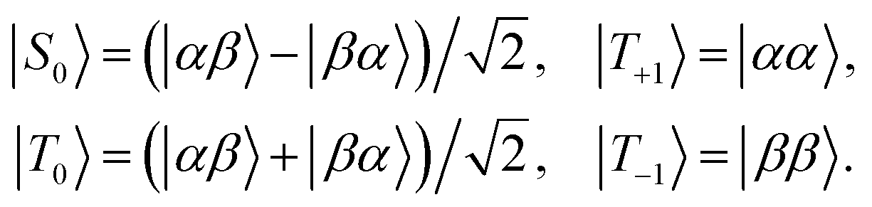 | (1) |
 | (2) |
In near-equivalent spin-pairs, defined by the condition |Δ| ≪ |J|, singlet order often exhibits a long lifetime without any further intervention, due to strong correlations in the fluctuating magnetic fields responsible for relaxation.35 In the intermediate coupling regime (|Δ| ∼ |J|), or the strong inequivalence regime (|Δ| ≫ |J|), on the other hand, singlet order only reveals its long-lived nature when it is “locked” or “sustained” by applying resonant radio-frequency fields.2,5,36 To a good approximation, the strong resonant radio-frequency field imposes magnetic equivalence on the effective spin Hamiltonian, so that the Hamiltonian eigenstates in the presence of the field are given, to a good approximation, by the singlet and triplet states defined in eqn (1).
In this article we quantify the inequivalence of the spin system by the singlet–triplet mixing angle θST, defined as follows
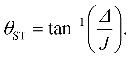 | (3) |
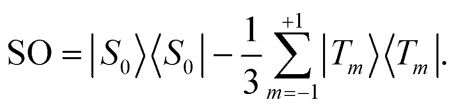
Singlet order is usually accessed by applying a radio-frequency pulse sequence which converts nuclear magnetisation along the field (represented by the operator Iz) into the singlet order operator of eqn (2). Several radio-frequency (rf) pulse sequences have been developed for this purpose.2,6,36–42 However, most pulse sequences are designed for either the near-equivalent regime (θST ≈ 0), or the strongly inequivalent regime (θST ≈ π/2). The intermediate coupling regime (θST ≈ π/4) is a difficult case which is not well-addressed by most existing sequences.
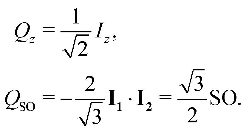
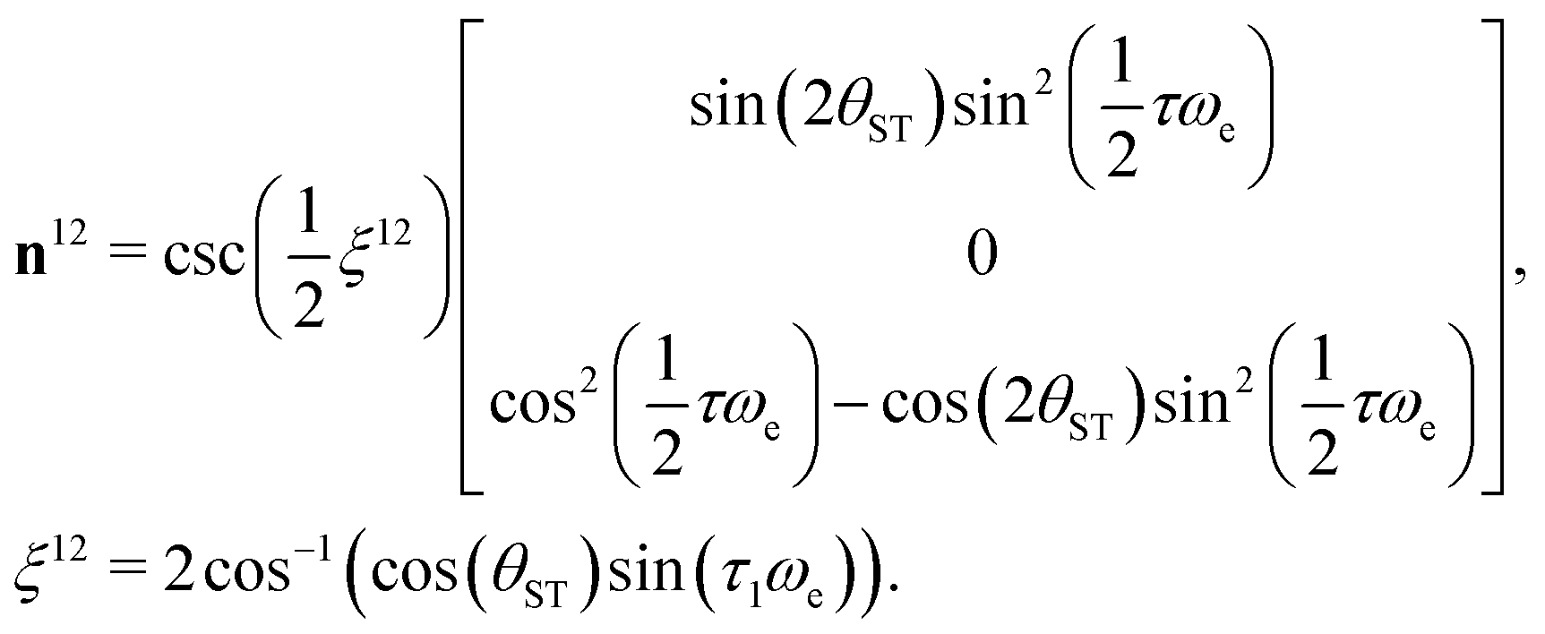
The normalised amplitude for the conversion of Zeeman order into singlet order is defined here as follows
| ζ = (QSO|ÛQz), | (4) |
 | (5) |
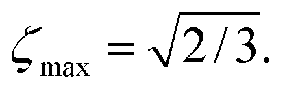
| |ζ| ≤ ζmax, | (6) |
 | (7) |
 of the normalised Zeeman order Qz into normalised singlet order QSO. In most cases, relaxation leads to further losses.
The magnetisation-to-singlet conversion amplitudes ζ are plotted against the singlet–triplet mixing angles for several different pulse sequences in Fig. 1.
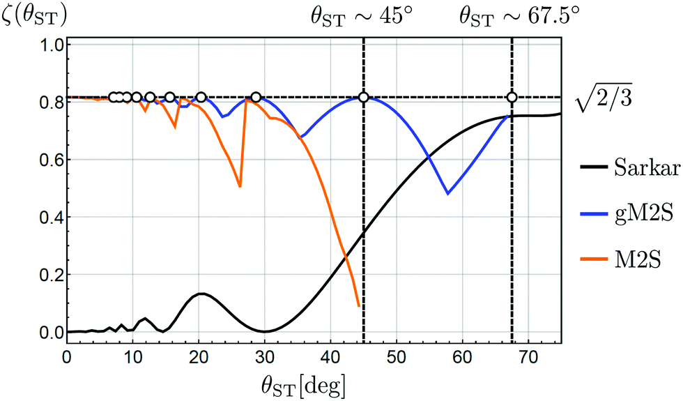 | ||
| Fig. 1 Transformation amplitudes ζ for Zeeman polarisation into singlet order (eqn (4)), as a function of mixing angle θST. The near-equivalent regime (θST ≈ 0) is shown on the left of the plot, with the strong inequivalence (weak coupling) regime (θST ≈ π/2) on the right, and the intermediate regime (θST ≈ π/4) in the middle. The transformation amplitudes ζ of the M2S,37 Sarkar46 and gM2S pulse sequences, are plotted. Relaxation is ignored in all cases. The pulse sequence parameters for the Sarkar sequence uses the analytic solutions in ref. 46. The pulse sequence parameters for the M2S and gM2S sequences use the analytic solutions in Table 1. Circles indicate the mixing angles θST for which the gM2S sequence provides optimal efficiency (ζ = ζmax). | ||
The magnetisation-to-singlet conversion amplitude of the M2S sequence37,38 is shown by the orange line. This simulation uses the optimum values for the M2S pulse sequence parameters given in Table 1 and described below.
 , and optimal echo number n* for the M2S and gM2S sequences
| M2S | gM2S | |
|---|---|---|
| θ ST | tan−1(Δ/J) | tan−1(Δ/J) |
| ω e |

|
|
| ξ 12 | 2![[thin space (1/6-em)]](https://www.rsc.org/images/entities/char_2009.gif) sin−1(Δ/J) sin−1(Δ/J) |

|
| n* | round(π/(2ξ12)) | round(π/ξ12) |
|
|
ω
e
−1cos−1(Δ(J − Δ)/(J(J + Δ))) |
|
|
|
The performance of M2S reaches the theoretical limit of ζ = ζmax in the near-equivalence regime (small values of θST). However the performance of M2S starts to oscillates when θST exceeds ∼20° and collapses completely for θST ≳ 40°. Other sequences for the near-equivalence regime, such as SLIC (spin-lock-induced crossing),40 also fail outside the near-equivalence regime.
The pulse sequence proposed by Sarkar et al.,46 on the other hand, has a performance shown by the black curve in Fig. 1. This sequence achieves near-optimal magnetisation-to-singlet conversion for θST ≳ 60° (strong inequivalence) but its performance declines steeply below θST ≲ 55°. Other proposed sequences for the strong-inequivalence regime2,6 have similar behaviour.
There have been several proposals for filling in the lacuna around θST ≈ 45°.
One approach is to introduce multiple-pulse chemical-shift scaling (CSS) into the magnetisation-to-singlet (M2S) pulse sequence.47 The resulting method is rather complex and involves the application of a large number of pulses. The sequence is prone to error accumulation and may give rise to sample heating.48
An alternative method is the homonuclear ADAPT (Alternating Delays Achieve Polarization Transfer) technique.49,50 This sequence consists of a repetitive sequence of short pulses. Simulations show that in ideal circumstances this sequence performs well for mixing angles given by 0 < θST ≲ 75°. However, ADAPT is not a robust method. As mentioned in ref. 50, the ADAPT sequence suffers from strong interference from off-resonance effects and radio-frequency field inhomogeneity. The performance of ADAPT is explored in more detail in the ESI.†
A different approach is to apply radio-frequency fields with computer-optimised variations of amplitude and phase to induce the required transformations. This includes the use of optimal control theory,51 and the set of techniques called APSOC (adiabatic passage spin-order conversion).41,42 Although such techniques are often efficient and robust, they have the disadvantage that there are no analytical solutions; in many cases, specific shapes must be derived for each set of spin system parameters. We do not consider these schemes further in this paper.
In this work we present a generalised M2S sequence (gM2S) which provides robust magnetisation-to-singlet transfer efficiency for systems ranging from near-equivalence well into the intermediate regime (0 < θST ≲ 67.5°). The parameters of the gM2S sequence are described by analytical equations for the case of infinitely short rf pulses. The performance of gM2S is shown by the blue line in Fig. 1. It covers the gap in performance between existing pulse sequences rather well, and, as discussed below, its performance is very robust with respect to common experimental imperfections.
2 Theory
2.1 Singlet–triplet evolution
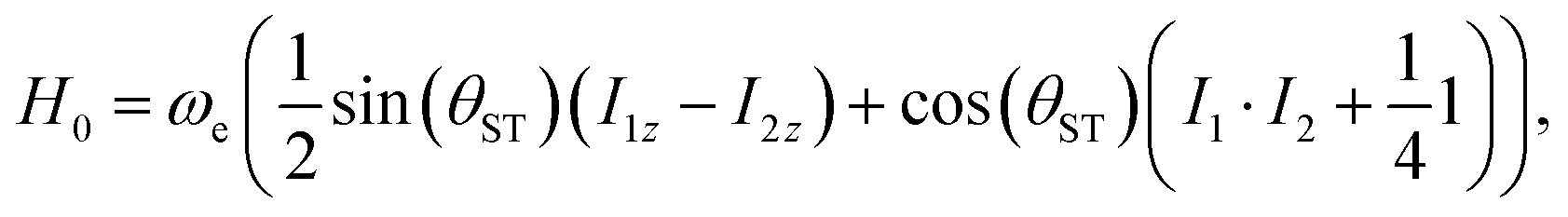
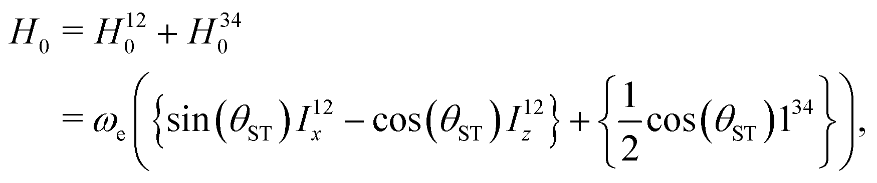
The rotating-frame Hamiltonian for a coupled two-spin-1/2 system in solution may be expressed as follows:52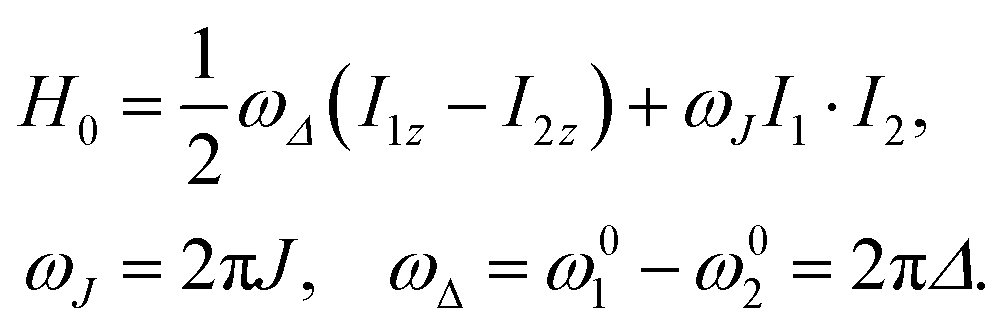 | (8) |
This suggests the following re-parametrisation of the Hamiltonian
 | (9) |
 | (10) |
Define a basis ![[scr B, script letter B]](https://www.rsc.org/images/entities/char_e13f.gif) spanned by the following basis states
spanned by the following basis states
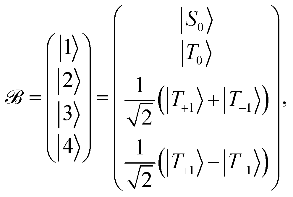 | (11) |
 | (12) |
 | (13) |
| Φrs(γ) = exp{ −iγ1rs}. | (14) |
2.2 Spin echoes
The sequences described below make extensive use of spin-echo (SE) blocks, of the form τ − 180y − τ, where τ denotes the duration of a delay interval. The propagator for a spin echo block is given by| USE(τ) = U0(τ)Ry(π)U0(τ). | (15) |
 | (16) |
| USE(τ) = U12SE(τ)U34SE(τ), | (17) |
 | (18) |
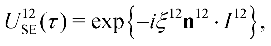 | (19) |
 | (20) |
2.3 The M2S sequence
The M2S pulse sequence is shown in Fig. 2. The sequence consists of 5 elements which operate as follows in the near-equivalence limit:37,38 (i) an initial 90y pulse converts longitudinal magnetisation into transverse magnetisation, corresponding to single-quantum coherences within the triplet manifold; (ii) a set of 2n consecutive spin echoes converts the single-quantum triplet–triplet coherences into coherences between the outer triplet states and the singlet state; (iii) a central 90x pulse generates a zero-quantum coherence between the central triplet state and the singlet state; (iv) a delay interval adjusts the phase of the zero-quantum coherence; (v) a final echo train converts the zero-quantum coherence into a population difference between the central triplet state and the singlet state. If all these elements work perfectly, the theoretical limit of is achieved for the magnetisation-to-singlet transformation amplitude (eqn (4)).
 | ||
| Fig. 2 (a) Magnetisation-to-Singlet (M2S) pulse sequence. (b) Singlet-to-Magnetisation (S2M) pulse sequence. The S2M sequence is defined here as the chronological reverse of the M2S sequence, including the final pulse. (c) Generalised Magnetisation-to-Singlet (gM2S) pulse sequence. (d) Generalised Singlet-to-Magnetisation (gS2M) pulse sequence. The gS2M sequence is defined as the chronological reverse of the gM2S sequence, including the final pulse. | ||
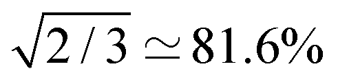
The S2M sequence is the chronological reverse of M2S (Fig. 4(b)). As defined here, M2S includes a final 90y pulse and converts singlet order back into z-magnetisation. The overall amplitude for converting z-magnetisation into singlet order by M2S, and back again into z-magnetisation by S2M, is given by ζ2max, which has the maximum achievable value of 2/3, for the case of unitary transformations.
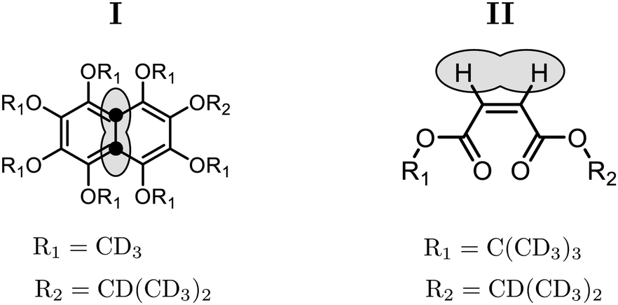 | ||
| Fig. 3 Chemical structures of compound (I) 1,2,3,4,5,6,8-heptakis(methoxy-d3)-7-((propan-2-yl-d7)oxy)-(4a,8a)-13C2-naphthalene and compound (II) 1-(iso-propyl-d7)-4-(tert-butyl-d9)-(Z)-but-2-enedioate. The spin pair used for the singlet NMR experiments is indicated by a lasso. Side-chain protons have been replaced by deuterons as indicated by R1 and R2. | ||
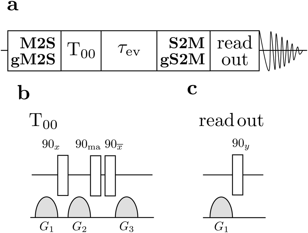 | ||
| Fig. 4 (a) General singlet NMR pulse sequence consisting of an M2S/gM2S block, a singlet order filtration element (T00), an evolution interval τev during which a continuous-wave (CW) rf field may be applied, an S2M/gS2M block, a read-out sequence for generating transverse magnetisation, and signal detection. (b) The singlet filter sequence consists of a set of radio-frequency pulses and field gradient pulses. The phase angle “ma” indicates the magic angle ≃54.7°.56 (c) The read out excitation sequence consists of a field gradient pulse for suppressing undesirable antiphase signal components, followed by excitation of transverse magnetisation by a 90y pulse. | ||
As originally described,37 the M2S delays τ1 and τ2, and the loop number n, are specified as follows:
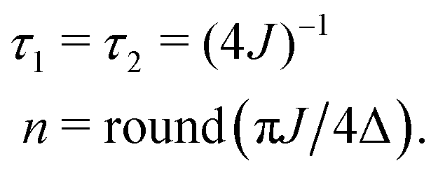 | (21) |
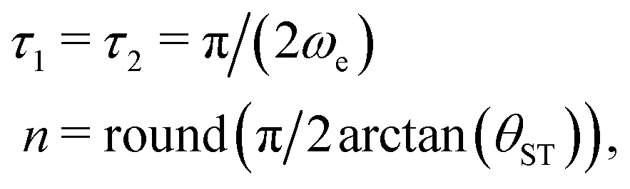 | (22) |
The M2S sequence includes two spin echo trains, before and after the central 90x pulse (see Fig. 2(a)). Ideally, these spin echo trains generate a rotation around the x-axis in the {|1〉,|2〉} subspace, through the angles of π (for the first spin echo train, consisting of 2n echoes) and π/2 (for the second spin echo train, consisting of n echoes). In both cases the rotation axis is ideally given by
 | (23) |
 | (24) |
 | (25) |
The total rotation angle of the second spin echo train ideally satisfies the condition
| nξ12 = π/2, | (26) |
| n* = round(π/(2ξ12)) | (27) |
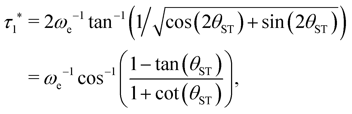
The two echo trains of the M2S sequence are separated by a 90x pulse followed by a free evolution interval of duration τ2. This evolution interval allows the singlet and central triplet states to come into phase.38 The derivation of the optimal evolution delay τ2* is straightforward but rather lengthy and is given in the ESI.† The result is
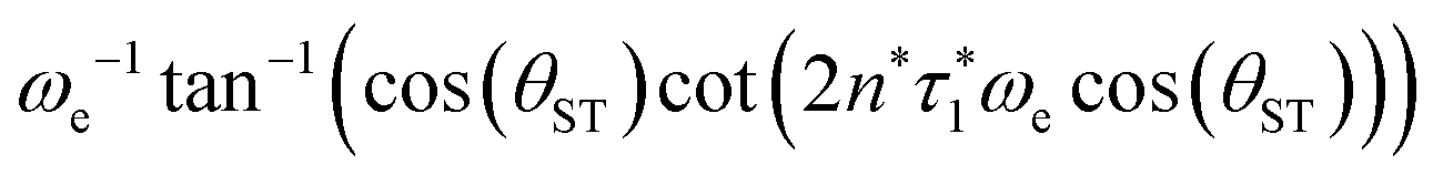
| τ2* =ωe−1tan−1(cos(θST)cot(2n*τ1*ωecos(θST))). | (28) |
The orange curve in Fig. 1 shows the predicted performance of M2S as a function of the singlet–triplet mixing angle θST, using the optimised M2S parameters summarized in Table 1. Simulations have also been performed for the literature solutions given in eqn (21) and eqn (22), and are not substantially different.
Fig. 1 shows that as θST increases from a low value, the performance of M2S oscillates in a saw-tooth fashion, with peaks at those values of mixing angles θST for which eqn (26) is satisfied exactly. Dips in performance are between these special values of θST.
Eqn (24) does not admit any physical solutions at all for θST ≥ π/4. This indicates a fundamental limitation of the M2S approach. In reality, as shown in Fig. 1, the performance of M2S declines steeply, well before the absolute cutoff at θST = π/4.
2.4 The gM2S sequence
The gM2S sequence is shown in Fig. 2(c). It is very similar to the M2S sequence, but with the initial 2n-fold echo block split into two n-fold echo blocks separated by a single 180y pulse. The optimal values of the delays τ1* and τ2* and the echo number n* are given in terms of the spin system parameters Δ and J in Table 1.For the M2S sequence, each spin echo element is designed to generate a rotation around the x-axis in the {|1〉,|2〉} subspace (eqn (23)). For the gM2S sequence, on the other hand, each spin echo element (τ1 − 180y − τ1) is designed to generate a rotation around a tilted axis in the {|1〉,|2〉} subspace of the form
 | (29) |
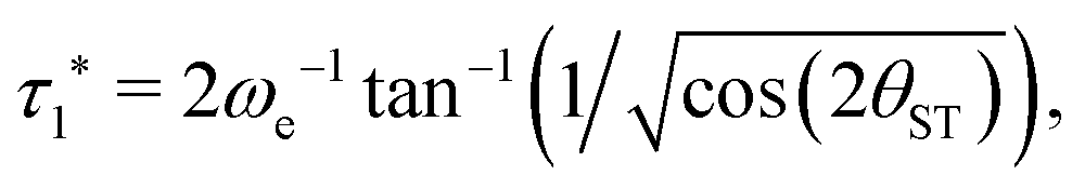
Eqn (29) is satisfied by choosing the following value for the optimal echo delay τ1*
 | (30) |
 . This condition allows physically realisable solutions for gM2S for a wide range of mixing angles 0 < θST < 3π/8. The upper limit of θST = 3π/8 = 67.5° is much larger than the M2S limit of θST = π/4 = 45°.
The effective rotation angle in the {|1〉,|2〉} subspace for the spin echo element (τ1* − 180y − τ1*) is given by
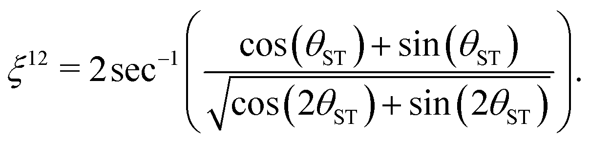 | (31) |
| n*ξ12 = π | (32) |
| n* = round(π/ξ12). | (33) |
If eqn (32) is satisfied exactly, the propagation operator in the {|1〉,|2〉} subspace for a sequence of n* spin echoes is given by
 | (34) |
 | (35) |
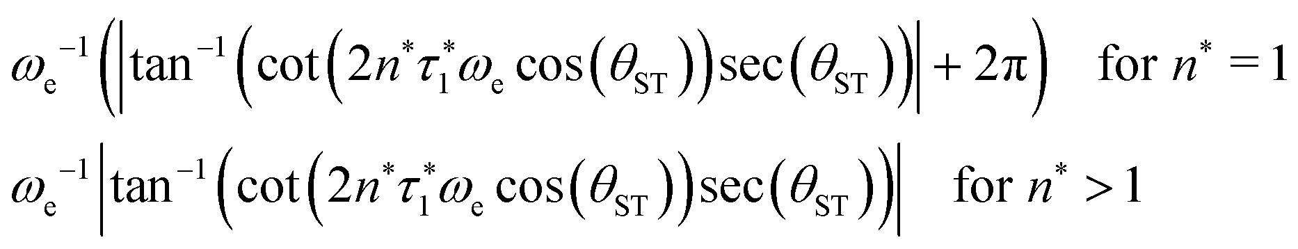
The rest of the gM2S sequence operates in the same way as the M2S sequence.37,38 However, the correct choice of the τ2 delay requires some detailed analysis, which is presented in the ESI.† The optimal value of the τ2 delay is given by
| τ2* =ωe−1|tan−1(cot(2n*τ1*ωecos(θST))sec(θST))| + 2πωe−1δ1n*, | (36) |
 | (37) |
The blue curve in Fig. 1 shows the performance of the gM2S sequence as a function of θST, with timing parameters specified in Table 1. The circles indicate singlet–triplet mixing angles at which eqn (32) is exactly satisfied for integer loop numbers n*. The gM2S sequence achieves the theoretical maximum transformation amplitude of  at those points, which include the centre of the intermediate regime at θST = π/4. There are dips in performance between these special values of θST, but the loss in amplitude is not severe. The gM2S sequence fills the gap between the M2S and Sarkar sequences by providing excitation efficiencies which are reasonably close to the theoretical maximum.
Since the gM2S sequence is based on spin echo sequences, it is very robust with respect to static field inhomogeneity, radiofrequency field inhomogeneity, and resonance offsets – especially when composite pulses are used. The performance of gM2S with respect to resonance offsets and rf field variations is explored in the ESI,† where it is contrasted with the ADAPT scheme.50
3 Experiments
Singlet NMR experiments were performed on solutions of two different compounds, in order to compare the performance of the gM2S and M2S sequences. Compound I is the 13C2-labelled naphthalene derivative shown in Fig. 3. This substance contains a near-equivalent 13C spin pair which supports singlet order with an exceptional lifetime in low magnetic field.57 Compound II is an asymmetric tert-butyl propyl maleate diester containing a magnetically inequivalent pair of 1H nuclei. Non participating side-chain protons are replaced by deuterons to reduce dipole–dipole relaxation contributions (see Fig. 3).3,5 The NMR parameters for the spin pairs in both compounds are summarised in Table 2.| Compound | I | II |
|---|---|---|
| Nucleus | 13C | 1H |
| J [Hz] | 54.10 | 12.30 |
| Δδ [ppm] | 0.061 | 0.024 |
| θ ST | 6.47° (@9.4 T) | 38.0° (@9.4 T) |
| T 1 [s] | 17.43 ± 0.20 | 8.69 ± 0.01 |
The synthesis of compound I is described in ref. 58. The experiments used a 0.1 M solution of compound I in deuterated acetone, contained in a 5 mm Wilmad LPV tube with the sample volume limited to 0.35 ml. The sample was degassed by several freeze–thaw-cycles. The synthesis of compound II is described in ref. 48. The experiments were performed on a degassed 1.7 mM solution in deuterated chloroform, with the sample volume restricted to 0.3 ml within a 5 mm Shigemi LPV tube to limit convection effects. The degassing procedure also consisted of several freeze–thaw-cycles.
All spectra were acquired at a magnetic field of 9.4 T. All pulses in Fig. 2 were replaced by their composite pulse counterparts to compensate for possible static and radio-frequency field inhomogeneities.59,60 Each 180y pulse was replaced by a composite inversion pulse of the form 90x180y90x.59 All 90ϕ pulses were replaced by the constant-rotation composite pulse 18097.2+ϕ360291.5+ϕ18097.2+ϕ90ϕ given in ref. 60. Individual data sets employed a basic two-step phase cycle and were averaged over two transients before post-processing using 0.25 Hz line broadening.
The general procedure for the singlet NMR experiments is shown in Fig. 4(a). Singlet order is generated using either a M2S or a gM2S sequence. This is followed by a singlet filtration step, denoted T00, which is implemented by a sequence of radio-frequency pulses and field gradients. This suppresses all signals not passing through singlet order.56 For singlet lifetime measurements an additional evolution interval τev is inserted, which may include the application of a spin-locking field. The singlet order is reconverted into z-magnetisation by applying a S2M or a gS2M pulse sequence (including the final 90y pulse, see Fig. 2(b and d)). The z-magnetisation is allowed to rest for a further delay which may include another field gradient pulse. This implements a z-filter which cleans up the final signal by removing undesirable signal components. A final 90y pulse induces transverse magnetisation and the NMR signal is detected.
The gM2S and M2S parameters were set by fixing the echo numbers to the values specified in Table 1 and optimising the delays τ1 and τ2 empirically in a small interval centred around the analytic solutions.
4 Results and discussion
4.1 Compound I
Singlet-filtered NMR signals for compound I are shown in Fig. 5(a), using the optimised M2S/S2M and gM2S/gS2M sequences. A simple pulse-acquire spectrum is also shown for reference. The pulse sequence parameters for the M2S and gM2S sequences are summarised in Table 3.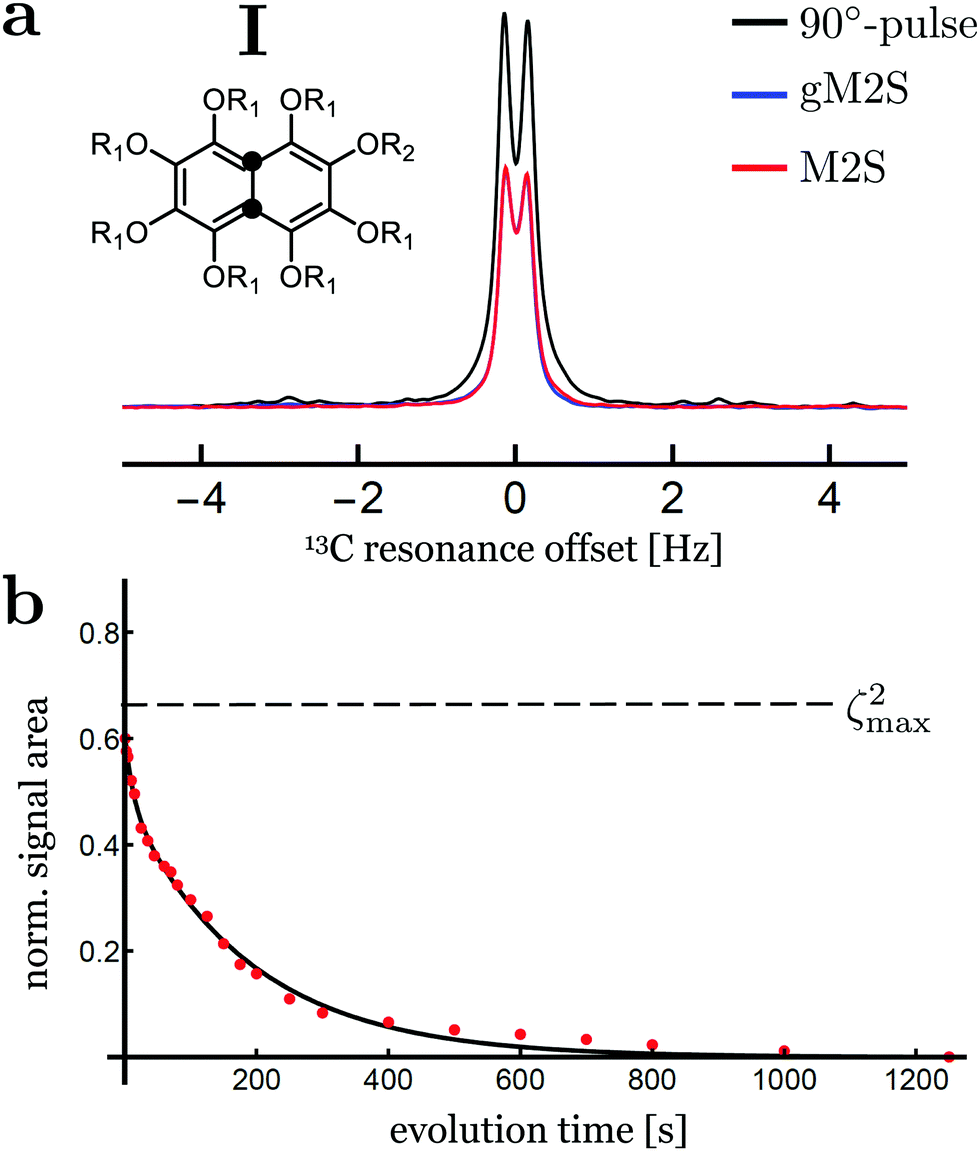 | ||
| Fig. 5 (a) Singlet-filtered 13C NMR spectra for compound I, using the M2S and gM2S sequences. A single pulse-acquire spectrum is shown for comparison. The spectra for M2S and gM2S are almost superimposed. (b) Singlet order decay as a function of the evolution interval τev, applying a spin-locking field with nutation frequency ∼2 kHz during the evolution interval. The plotted signal amplitude is normalised against the single-pulse-acquire spectrum. The solid line shows the best fit to a bi-exponential decay. The theoretical maximum of ζ2max = 2/3 is indicated by the horizontal dashed line. | ||
| M2S | gM2S | |
|---|---|---|
| n* = nexp | 7 | 11 |
| τ 1* [ms] | 4.64 | 4.33 |
| τ exp1 [ms] | 4.63 | 4.33 |
| τ 2* [ms] | 4.48 | 1.86 |
| τ exp2 [ms] | 4.63 | 2.37 |
| ω nut/2π [kHz] | 30.0 | 30.0 |
The M2S and gM2S sequences display very similar performance, as expected for the near-equivalence regime. Integration of the resulting spectra and comparison with the pulse-acquire reference indicates that both sequences pass approximately 60% of the initial magnetisation through singlet order and back to magnetisation (ζ2 ≃ 60% for M2S and 59% for gM2S). This is respectably close to the theoretical maximum of ζ2max = 2/3 ≃ 66.7%. The remaining loss may be attributed to relaxation during the pulse sequences and residual pulse imperfections.
Fig. 5(b) shows the decay of singlet order for compound I using the gM2S/gS2M sequence with 2 kHz continuous-wave irradiation during the evolution interval. The decay curve displays a bi-exponential behaviour of the form: s(τev) = A1exp(−τev/T1) + ASexp(−τev/TS) with fit parameters A1 = 0.12 ± 1.6, AS = 0.49 ± 0.02, T1 = 12.2 ± 4.1 s and TS = 186 ± 9 s. The major component may be identified as long-lived singlet order with a relaxation time constant of TS ≃ 186 s, which is approximately 10 times longer than the longitudinal relaxation time constant T1 = 17.4 ± 0.2 s. Comparable results have been reported previously at this magnetic field, albeit using the M2S sequence instead of the gM2S sequence.57
At this stage the bi-exponential decay behaviour of singlet order in compound I is not fully understood. A possible explanation may involve the weak scalar couplings to nearby deuterons. These are known to induce scalar relaxation of the second kind (SR2K) resulting in a non-mono-exponential decay.61 Since the sample volume of compound I was not restricted, convection effects could also contribute to the bi-exponential decay behaviour.62
4.2 Compound II
The spectra for compound II after singlet order excitation via M2S and gM2S are shown in Fig. 6(a). The experimentally optimised M2S and gM2S parameters are given in Table 4.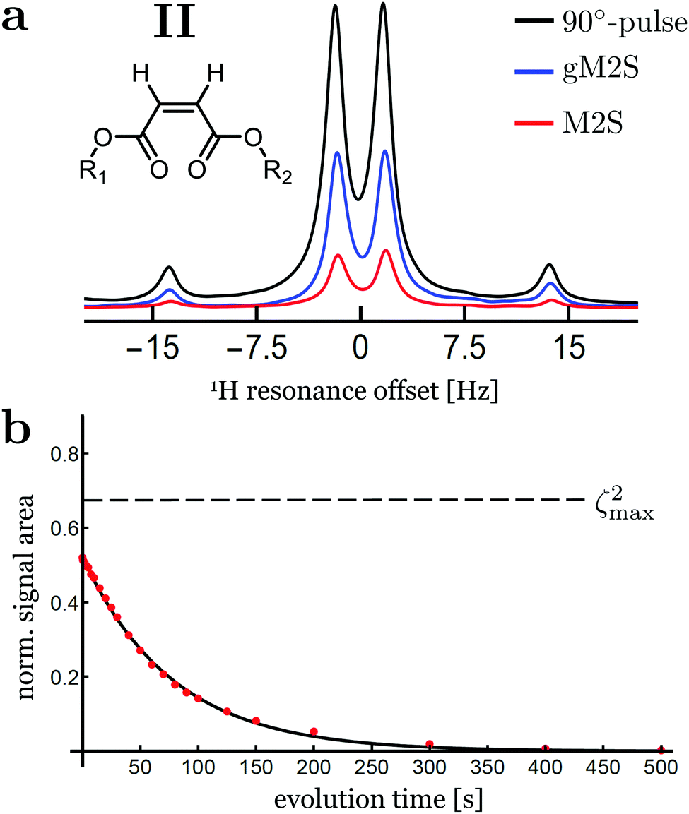 | ||
| Fig. 6 (a) Singlet-filtered 1H NMR spectra for compound II, using the M2S and gM2S sequences. A single pulse-acquire spectrum is shown for comparison. (b) Singlet order decay as a function of the evolution interval τev, applying a spin-locking field with nutation frequency ∼2 kHz during the evolution interval. The plotted signal amplitudes are normalised against the single-pulse-acquire spectrum. The solid line shows the best fit to an exponential decay. The theoretical maximum of ζ2max = 2/3 is indicated by the horizontal dashed line. | ||
| M2S | gM2S | |
|---|---|---|
| n* = nexp | 1 | 2 |
| τ 1* [ms] | 23.46 | 14.30 |
| τ exp1 [ms] | 21.80 | 15.40 |
| τ 2* [ms] | 11.16 | 1.20 |
| τ exp2 [ms] | 12.50 | 1.24 |
| ω nut/2π [kHz] | 25.0 | 25.0 |
The proton spin system of compound II has a singlet–triplet mixing angle of θST = 38.0°, which places it firmly in the intermediate-coupling regime. In this case a large differences in performance is observed for the M2S and gM2S sequences.
The signal amplitude observed for the M2S sequence is weak for this system, with an integrated amplitude of only ∼19% of the pulse-acquire spectrum.
The gM2S sequence gives a much stronger singlet-filtered NMR signal. The integrated amplitude of the singlet-filtered NMR spectrum is ∼50% of the pulse-acquire spectrum, which is a respectable fraction of the theoretical maximum, ζ2max = 2/3 ≃ 66.7%.
The decay of singlet order for compound II under 2 kHz continuous wave irradiation is shown in Fig. 6(b). The decay curve is well approximated by a mono-exponential decay of the form: s(τev) = ASexp(−τev/TS) with fit parameters AS = 0.52 ± 0.02 and TS = 77.6 ± 1.0 s. The singlet order decay constant for compound II is therefore approximately ten times longer than the time constant for thermalisation of longitudinal magnetisation, T1 = 8.69 ± 0.01 s.
5 Conclusions
To summarise, we have described a generalisation of the singlet-to-magnetisation (M2S) sequence. The proposed generalised-M2S sequence (gM2S) performs near-optimal singlet order excitation for spin-pair systems ranging from the near-equivalence limit, through the intermediate regime, to the boundary of strong inequivalence. We have given analytical solutions for the delays and loop numbers in the short-pulse limit. Small adjustments for finite pulse durations are readily implemented by empirical optimisation on the spectrometer.The performance of M2S and gM2S was evaluated experimentally in two model systems, containing spin-1/2 pairs in the near-equivalence and intermediate coupling regimes. In the near-equivalence regime, both M2S and gM2S achieve near-optimal efficiency for the passage of transverse magnetisation through singlet order and back to transverse magnetisation. In the intermediate coupling regime, on the other hand, the gM2S sequence greatly outperforms the M2S sequence.
Although the implementation of gM2S is somewhat more complex than M2S, the gM2S overcomes the restriction of the M2S to near-equivalent systems and enables the study of new molecular systems.37,38 We therefore anticipate its incorporation into a wide class of singlet-assisted NMR experiments.15–17,25–28,31–34
Further extensions to the case of heteronuclear spin systems are feasible, for example in the context of parahydrogen-enhanced NMR.63–65
Conflicts of interest
There are no conflicts to declare.Acknowledgements
This research was supported by the European Research Council (786707-FunMagResBeacons) and the Engineering and Physical Sciences Research Council (EPSRC-UK), grant numbers EP/P009980/1 and EP/P030491/1. A. J. acknowledges funding from the National Science Foundation under award #CHE 1710046 and a Diamond Jubilee Visiting Fellowship from the University of Southampton.References
- M. Carravetta, O. G. Johannessen and M. H. Levitt, Phys. Rev. Lett., 2004, 92, 153003 CrossRef PubMed.
- M. Carravetta and M. H. Levitt, J. Am. Chem. Soc., 2004, 126, 6228–6229 CrossRef CAS PubMed.
- M. Carravetta and M. H. Levitt, J. Chem. Phys., 2005, 122, 214505 CrossRef PubMed.
- M. H. Levitt, Annu. Rev. Phys. Chem., 2012, 63, 89–105 CrossRef CAS PubMed.
- G. Pileio and M. H. Levitt, J. Chem. Phys., 2009, 130, 214501 CrossRef PubMed.
- G. Pileio, M. Carravetta, E. Hughes and M. H. Levitt, J. Am. Chem. Soc., 2008, 130, 12582–12583 CrossRef CAS PubMed.
- G. Stevanato, J. T. Hill-Cousins, P. Håkansson, S. S. Roy, L. J. Brown, R. C. D. Brown, G. Pileio and M. H. Levitt, Angew. Chem., Int. Ed., 2015, 54, 3740–3743 CrossRef CAS PubMed.
- T. Theis, G. X. Ortiz, A. W. J. Logan, K. E. Claytor, Y. Feng, W. P. Huhn, V. Blum, S. J. Malcolmson, E. Y. Chekmenev, Q. Wang and W. S. Warren, Sci. Adv., 2016, 2, e1501438 CrossRef PubMed.
- S. J. Elliott, P. Kadeřávek, L. J. Brown, M. Sabba, S. Glöggler, D. J. O'Leary, R. C. D. Brown, F. Ferrage and M. H. Levitt, Mol. Phys., 2019, 117, 861–867 CrossRef CAS.
- M. H. Levitt, J. Magn. Reson., 2019, 306, 69–74 CrossRef CAS PubMed.
- N. Salvi, Annual Reports on NMR Spectroscopy, Academic Press, 2019, vol. 96, pp. 1–33 Search PubMed.
- J.-N. Dumez, Mol. Phys., 2019, 1–11 Search PubMed.
- S. Cavadini, J. Dittmer, S. Antonijevic and G. Bodenhausen, J. Am. Chem. Soc., 2005, 127, 15744–15748 CrossRef CAS PubMed.
- G. Pileio, J.-N. Dumez, I.-A. Pop, J. T. Hill-Cousins and R. C. D. Brown, J. Magn. Reson., 2015, 252, 130–134 CrossRef CAS PubMed.
- S. Cavadini and P. R. Vasos, Concepts Magn. Reson., Part A, 2008, 32, 68–78 CrossRef.
- G. Pileio and S. Ostrowska, J. Magn. Reson., 2017, 285, 1–7 CrossRef CAS PubMed.
- M. C. Tourell, I.-A. Pop, L. J. Brown, R. C. D. Brown and G. Pileio, Phys. Chem. Chem. Phys., 2018, 20, 13705–13713 RSC.
- L. Buljubasich, M. B. Franzoni, H. W. Spiess and K. Münnemann, J. Magn. Reson., 2012, 219, 33–40 CrossRef CAS PubMed.
- T. Theis, M. Truong, A. M. Coffey, E. Y. Chekmenev and W. S. Warren, J. Magn. Reson., 2014, 248, 23–26 CrossRef CAS PubMed.
- Y. Zhang, P. C. Soon, A. Jerschow and J. W. Canary, Angew. Chem., Int. Ed., 2014, 53, 3396–3399 CrossRef CAS PubMed.
- Y. Zhang, K. Basu, J. W. Canary and A. Jerschow, Phys. Chem. Chem. Phys., 2015, 17, 24370–24375 RSC.
- S. S. Roy, P. J. Rayner, P. Norcott, G. G. R. Green and S. B. Duckett, Phys. Chem. Chem. Phys., 2016, 18, 24905–24911 RSC.
- S. S. Roy, P. Norcott, P. J. Rayner, G. G. R. Green and S. B. Duckett, Chem. – Eur. J., 2017, 23, 10496–10500 CrossRef CAS PubMed.
- S. S. Roy, G. Stevanato, P. J. Rayner and S. B. Duckett, J. Magn. Reson., 2017, 285, 55–60 CrossRef CAS PubMed.
- K. F. Sheberstov, H.-M. Vieth, H. Zimmermann, B. A. Rodin, K. L. Ivanov, A. S. Kiryutin and A. V. Yurkovskaya, Sci. Rep., 2019, 9, 1–11 CrossRef PubMed.
- A. S. Kiryutin, B. A. Rodin, A. V. Yurkovskaya, K. L. Ivanov, D. Kurzbach, S. Jannin, D. Guarin, D. Abergel and G. Bodenhausen, Phys. Chem. Chem. Phys., 2019, 21, 13696–13705 RSC.
- W. Iali, S. S. Roy, B. J. Tickner, F. Ahwal, A. J. Kennerley and S. B. Duckett, Angew. Chem., 2019, 131, 10377–10381 CrossRef.
- S. S. Roy, P. J. Rayner, M. J. Burns and S. B. Duckett, J. Chem. Phys., 2020, 152, 014201 CrossRef PubMed.
- N. Salvi, R. Buratto, A. Bornet, S. Ulzega, I. Rentero Rebollo, A. Angelini, C. Heinis and G. Bodenhausen, J. Am. Chem. Soc., 2012, 134, 11076–11079 CrossRef CAS PubMed.
- R. Buratto, D. Mammoli, E. Chiarparin, G. Williams and G. Bodenhausen, Angew. Chem., Int. Ed., 2014, 53, 11376–11380 CrossRef CAS PubMed.
- W. Iali, P. J. Rayner and S. B. Duckett, Sci. Adv., 2018, 4, eaao6250 CrossRef PubMed.
- A. Sadet, C. Stavarache, F. Teleanu and P. R. Vasos, Sci. Rep., 2019, 9, 1–7 CrossRef CAS PubMed.
- S. Yang, J. McCormick, S. Mamone, L.-S. Bouchard and S. Glöggler, Angew. Chem., Int. Ed., 2019, 58, 2879–2883 CrossRef CAS PubMed.
- T. Kress, A. Walrant, G. Bodenhausen and D. Kurzbach, J. Phys. Chem. Lett., 2019, 10, 1523–1529 CrossRef CAS PubMed.
- G. Pileio, Prog. Nucl. Magn. Reson. Spectrosc., 2010, 56, 217–231 CrossRef CAS PubMed.
- R. Sarkar, P. Ahuja, D. Moskau, P. R. Vasos and G. Bodenhausen, ChemPhysChem, 2007, 8, 2652–2656 CrossRef CAS PubMed.
- G. Pileio, M. Carravetta and M. H. Levitt, Proc. Natl. Acad. Sci. U. S. A., 2010, 107, 17135–17139 CrossRef CAS PubMed.
- M. C. D. Tayler and M. H. Levitt, Phys. Chem. Chem. Phys., 2011, 13, 5556–5560 RSC.
- R. Sarkar, P. Ahuja, P. R. Vasos and G. Bodenhausen, Phys. Rev. Lett., 2010, 104, 053001 CrossRef PubMed.
- S. J. DeVience, R. L. Walsworth and M. S. Rosen, Phys. Rev. Lett., 2013, 111, 173002 CrossRef PubMed.
- A. N. Pravdivtsev, A. S. Kiryutin, A. V. Yurkovskaya, H.-M. Vieth and K. L. Ivanov, J. Magn. Reson., 2016, 273, 56–64 CrossRef CAS PubMed.
- B. A. Rodin, K. F. Sheberstov, A. S. Kiryutin, J. T. Hill-Cousins, L. J. Brown, R. C. D. Brown, B. Jamain, H. Zimmermann, R. Z. Sagdeev, A. V. Yurkovskaya and K. L. Ivanov, J. Chem. Phys., 2019, 150, 064201 CrossRef PubMed.
- J. Jeener, Advances in Magnetic and Optical Resonance, Academic Press, 1982, vol. 10, pp. 1–51 Search PubMed.
- O. W. Sørensen, J. Magn. Reson., 1990, 86, 435–440 Search PubMed.
- M. H. Levitt, J. Magn. Reson., 2016, 262, 91–99 CrossRef CAS PubMed.
- R. Sarkar, P. R. Vasos and G. Bodenhausen, J. Am. Chem. Soc., 2007, 129, 328–334 CrossRef CAS PubMed.
- G. A. Morris, N. P. Jerome and L.-Y. Lian, Angew. Chem., Int. Ed., 2003, 42, 823–825 CrossRef CAS PubMed.
- B. Kharkov, X. Duan, E. S. Tovar, J. W. Canary and A. Jerschow, Phys. Chem. Chem. Phys., 2019, 21, 2595–2600 RSC.
- G. Stevanato, J. Magn. Reson., 2017, 274, 148–162 CrossRef CAS PubMed.
- S. J. Elliott and G. Stevanato, J. Magn. Reson., 2019, 301, 49–55 CrossRef CAS PubMed.
- C. Laustsen, S. Bowen, M. S. Vinding, N. C. Nielsen and J. H. Ardenkjaer-Larsen, Magn. Reson. Med., 2014, 71, 921–926 CrossRef PubMed.
- M. H. Levitt, Spin dynamics: basics of nuclear magnetic resonance, Wiley, 2001 Search PubMed.
- S. Vega and A. Pines, J. Chem. Phys., 1977, 66, 5624–5644 CrossRef CAS.
- S. Vega, J. Chem. Phys., 1978, 68, 5518–5527 CrossRef CAS.
- S. Scherer, Symmetrien und Gruppen in der Teilchenphysik, Springer Spektrum, 2016 Search PubMed.
- M. C. D. Tayler and M. H. Levitt, J. Am. Chem. Soc., 2013, 135, 2120–2123 CrossRef CAS PubMed.
- G. Stevanato, S. S. Roy, J. Hill-Cousins, I. Kuprov, L. J. Brown, R. C. D. Brown, G. Pileio and M. H. Levitt, Phys. Chem. Chem. Phys., 2015, 17, 5913–5922 RSC.
- J. T. Hill-Cousins, I.-A. Pop, G. Pileio, G. Stevanato, P. HÅkansson, S. S. Roy, M. H. Levitt, L. J. Brown and R. C. D. Brown, Org. Lett., 2015, 17, 2150–2153 CrossRef CAS PubMed.
- M. H. Levitt and R. Freeman, J. Magn. Reson., 1979, 33, 473–476 Search PubMed.
- S. Wimperis, J. Magn. Reson., Ser. A, 1994, 109, 221–231 CrossRef CAS.
- S. J. Elliott, C. Bengs, L. J. Brown, J. T. Hill-Cousins, D. J. O'Leary, G. Pileio and M. H. Levitt, J. Chem. Phys., 2019, 150, 064315 CrossRef CAS PubMed.
- B. Kharkov, X. Duan, J. W. Canary and A. Jerschow, J. Magn. Reson., 2017, 284, 1–7 CrossRef CAS PubMed.
- S. Kadlecek, K. Emami, M. Ishii and R. Rizi, J. Magn. Reson., 2010, 205, 9–13 CrossRef CAS PubMed.
- J. Eills, G. Stevanato, C. Bengs, S. Glöggler, S. J. Elliott, J. Alonso-Valdesueiro, G. Pileio and M. H. Levitt, J. Magn. Reson., 2017, 274, 163–172 CrossRef CAS PubMed.
- J. Eills, J. Blanchard, T. Wu, C. Bengs, J. Hollenbach, D. Budker and M. Levitt, Polarization Transfer via Field Sweeping in Parahydrogen-Enhanced Nuclear Magnetic Resonance, ChemRxiv, 2019.
Footnote |
| † Electronic supplementary information (ESI) available. See DOI: 10.1039/d0cp00935k |
| This journal is © the Owner Societies 2020 |