
 Open Access Article
 This Open Access Article is licensed under a
 Creative Commons Attribution 3.0 Unported Licence
Revisiting nuclear tunnelling in the aqueous ferrous–ferric electron transfer†
Wei
Fang‡
 ,
Rhiannon A.
Zarotiadis‡
and
Jeremy O.
Richardson
*
,
Rhiannon A.
Zarotiadis‡
and
Jeremy O.
Richardson
*
Laboratory of Physical Chemistry, ETH Zürich, 8093 Zürich, Switzerland. E-mail: jeremy.richardson@phys.chem.ethz.ch
First published on 5th February 2020
Abstract
The aqueous ferrous–ferric system provides a classic example of an electron-transfer process in solution. There has been a long standing argument spanning more than three decades around the importance of nuclear tunnelling in this system, with estimates based on Wolynes theory suggesting a quantum correction factor of 65, while estimates based on a related spin-boson model suggest a smaller factor of 7–36. Recently, we have shown that Wolynes theory can break down for systems with multiple transition states leading to an overestimation of the rate, and we suggest that a liquid system such as the one investigated here may be particularly prone to this. We re-investigate this old yet interesting system with the first application of the recently developed golden-rule quantum transition-state theory (GR-QTST). We find that GR-QTST can be applied to this complex system without apparent difficulties and that it gives a prediction for the quantum rate 6 times smaller than that from Wolynes theory. The fact that these theories give different results suggests that although it is well known that the system can be treated using linear response and therefore resembles a spin-boson model in the classical limit, this approximation is questionable in the quantum case. It also intriguingly suggests the possibility that the previous predictions were overestimating the rate due to a break down of Wolynes theory.
Introduction
The realms of chemistry and biology serve us with a colourful variety of reactions affected by nuclear tunnelling.1 In chemistry, tunnelling is predicted to be important under a wide range of conditions from astrochemical reactions occurring on cosmic dust2 and nuclear fusion in stars3 to organic chemistry, where even heavy-atom tunnelling has been identified.4,5 Biological systems have also been suspected of employing nuclear tunnelling, for instance in photosynthesis taking place in bacteria6 or during enzyme catalysis.7,8 To resolve such controversial hypotheses, a reliable method to calculate effects of nuclear tunnelling is clearly desirable. Such a theory will be useful to quantify the relevance of tunnelling in a given reaction.In this work we focus specifically on the case of electron-transfer reactions.9–11 These reactions are nonadiabatic and governed by a change of electronic state and one cannot therefore employ the Born–Oppenheimer approximation.12 The rate is however well described by Fermi's golden rule,13,14 although in practice this cannot be evaluated for complex molecular systems as it requires complete knowledge of the internal eigenstates of the system. The simplest approach is to map the system onto a harmonic spin-boson model, for which the rate can be evaluated exactly. The mapping is of course not exact, and thus this procedure involves an uncontrolled approximation.
Modern quantum rate theories15 are typically based on the path-integral approach to quantum mechanics,16 which allows tunnelling and other nuclear quantum effects (NQEs) to be included efficiently into molecular simulations17 using a quantum-classical correspondence.18 However, because the rate is not defined as a simple expectation value of the density matrix, but rather in terms of a time correlation function,19 it is by no means trivial to calculate rates in this way and further approximations are required. In this paper, we will concentrate in particular on quantum transition-state theories and not consider dynamical methods.20,21
Semiclassical instanton rate theory22–24 predicts the tunnelling rate and mechanism via locating the optimal tunnelling pathway (the instanton) defined by a stationary-action principle. Based on a similar first-principles derivation as in the normal regime,25,26 instanton theory has been extended to treat electron-transfer reactions27–29 in both the normal and inverted regimes.30 It has the most rigorous derivation of the methods discussed in this paper, shows excellent agreement with exact methods on model systems and is well suited for gas-phase electron-transfer reactions. However, for liquid systems, it is formally not valid to apply instanton theory,26 although in some cases approximate application is possible by using an implicit solvent model or by freezing all atoms not expected to be involved in tunnelling at the transition state (TS) geometry.31 For the general case, an extension of instanton theory that allows for sampling is desired.
Wolynes theory32 is an approximate quantum rate theory which describes electron transfer in Fermi's golden-rule limit. It is defined in terms of path integrals which can be evaluated using an N-bead discretisation with each bead assigned to either the reactant or product electronic state. The method of path-integral molecular dynamics (PIMD)33 opens Wolynes theory up to the sampling tools of molecular dynamics (MD) calculations and accordingly makes it a computationally feasible approach for simulating atomistic systems.34–36 Lawrence and Manolopoulos have recently shown that Wolynes theory can also be successfully extrapolated to the Marcus inverted regime.37
Wolynes theory has been thoroughly investigated not only for atomistic but also for model systems such as the spin-boson model, where it compares very well to exact results,34,38 because it recovers the stationary phase-approximation.39 A limitation to Wolynes theory however is that it does not tend to the classical limit for anharmonic systems.28,40 Recently, we have also pointed out another crucial limitation of Wolynes theory, which is that its approximations break down when a system consists of two or more transition states.41 This break-down can manifest itself as an overestimation of the reaction rate by more than an order of magnitude in either the classical or the quantum limit. This may lead to the prediction of an artificial tunnelling factor. The break-down of Wolynes theory can be related to its lack of connection to instanton theory, as it is observed that it does not necessarily sample paths close to the diabatic crossing seam, where the instantons are located, but can rather include unphysical configurations far from the seam. This makes any mechanistic insight or a correct rate prediction impossible.
The quantum-instanton method42 suffers in a similar way when applied to strongly asymmetric barriers, which can be explained from an analysis in terms of semiclassical pathways and corrected by introducing a projection to connect it to the instanton.43 A further example to back this line of argumentation is the success of ring-polymer molecular dynamics (RPMD),44–46 which was shown to be closely connected to the semiclassical instanton rate theory in the deep-tunnelling regime.47 Standard RPMD rate theory is only applicable in the adiabatic limit,48–50 but has also been used to study electron tunnelling (instead of NQEs) in the aqueous ferrous–ferric system.51 Building on the success of adiabatic RPMD rate theory, attempts were made to extend it to treat the nonadiabatic limit. Two such attempts are the kinetically-constrained RPMD52–54 and the isomorphic RPMD method,55,56 which do not always give reliable tunnelling factors.57,58 One can in turn relate this behaviour to their lack of connection to instanton theory.
We therefore proposed golden-rule quantum transition-state theory (GR-QTST)40 in order to overcome issues of possible break-down behaviour by keeping a relation to instanton theory, but also retain the advantageous feature of Wolynes theory which includes not only the instanton but also paths in its vicinity. This method is computed in a similar way to Wolynes theory, except that a constraint is imposed on the sampled paths such that the energy on the reactant and product states must match. Adding such a constraint has been proposed as a general approach for defining quantum transition-state theories.59 This constraint is automatically obeyed by all instantons, which ensures a strong connection to instanton theory, and it also retains the correct classical limit. GR-QTST has been shown to perform very well for model systems in both the normal and inverted regimes,40 including the multidimensional spin-boson model. GR-QTST was also investigated for systems with multiple transition states, where Wolynes theory breaks, and provides accurate rate predictions.41 For the systems tested so far, we claimed it was the most accurate imaginary-time path-integral method currently available. However, GR-QTST has not previously been applied to atomistic simulations. This work therefore aims to investigate the applicability of GR-QTST as well as to see what physical insights it can offer by revisiting the early papers on the aqueous ferrous–ferric electron transfer.34,60,61 This is a prototypical atomistic system for which a computationally inexpensive force field is readily available.60 The seemingly simple interactions in this system forge a rough, high-dimensional, anharmonic potential energy surface (PES) and display high levels of complexity due to it being atomistic, which is more realistic and complex far beyond any of the models previously studied by GR-QTST.
The system is depicted in Fig. 1, and despite its seemingly innocent appearance, there has been a long standing argument over the importance of nuclear tunnelling in this system at room temperature. The quantum correction factor reported in ref. 34 and calculated based on similar ideas to Wolynes theory is approximately 65, suggesting a significant contribution from nuclear tunnelling. This estimate is significantly larger (∼6 times) than other predictions made at the time.62 Due to this discrepancy in the calculated tunnelling enhancements, the aqueous ferrous–ferric system is a good atomistic test case worth revisiting with newly developed rate theories. It is also of interest to investigate the applicability of Wolynes theory in this case in view of a possible overestimation of the nuclear tunnelling effect.
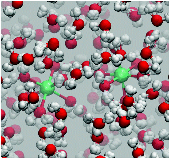 | ||
| Fig. 1 Snapshot of the aqueous ferrous–ferric system from a PIMD trajectory. The Fe2+ and Fe3+ ions are shown in green and are solvated in an octahedral ligand environment. | ||
In order to reexamine the earlier findings of Chandler and co-workers34,60 and add the investigation of GR-QTST for this system, we recapitulate the various rate theories under study in Section 2. The computational details of the implementation of each rate theory are given in Section 3 and the results are presented and discussed in Section 4. We conclude in Section 5 on the quality and appropriateness of the various quantum rate theories and discuss our work in the context of that of others.
Theory
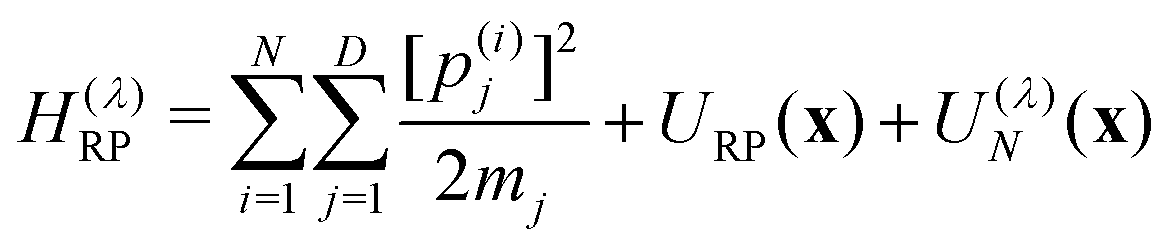
The quantum Hamiltonian describing an electron-transfer reaction is12| Ĥ = Ĥ0|0〉〈0| + Ĥ1|1〉〈1| + Δ(|0〉〈1| + |1〉〈0|), | (1) |
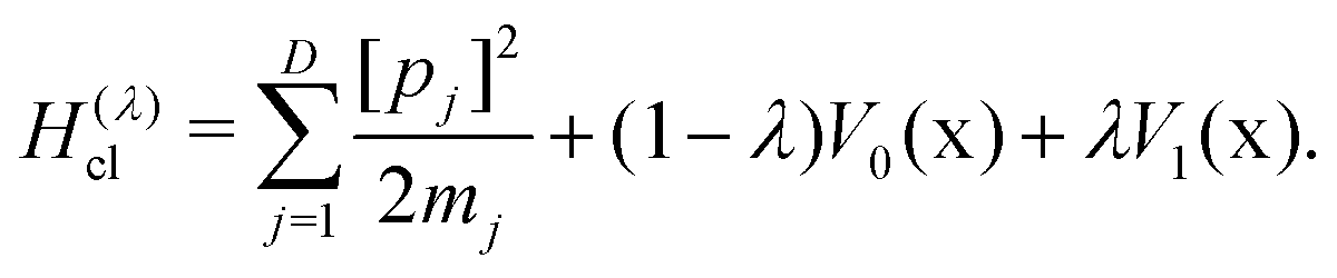
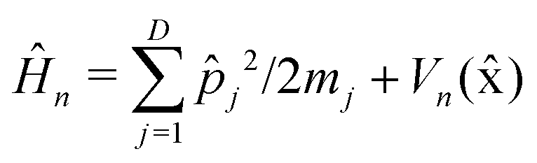 is the nuclear Hamiltonian for the electronic state n with the PES Vn(x), where x = (x1,…,xD) is the nuclear geometry and the index j runs over each of the D nuclear degrees of freedom of the system with momentum pj and associated mass mj. Following the work of Chandler and co-workers,34Δ is assumed to be a constant, which is known as the Condon approximation.
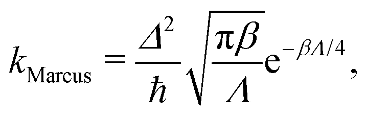
The rate, in the limit of small Δ, is in principle given by Fermi's golden rule,13 which is commonly approximated using Marcus theory.10 For a symmetric system, the rate is then given by a simple equation:
 | (2) |
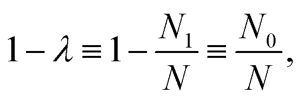
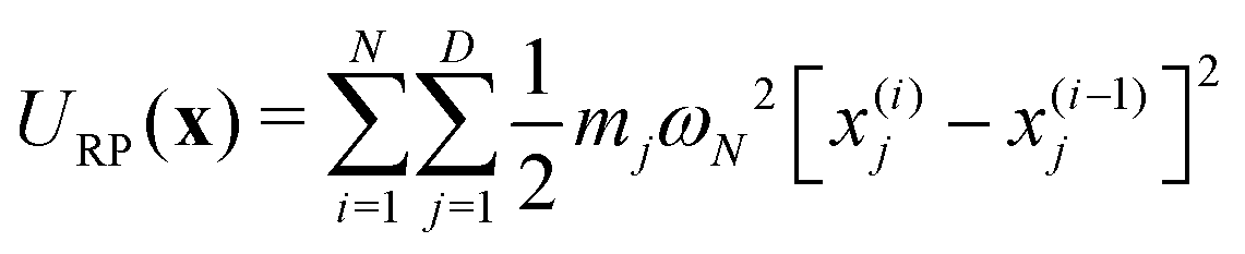
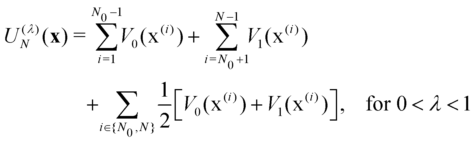
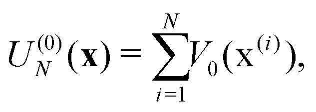
In electron-transfer theory, cyclic paths are formed by joining together an open-ended path on the reactant state and an open-ended path on the product state. For a ring-polymer representation of these paths, we introduce λ as a dimensionless order parameter, which determines how the ring-polymer beads are distributed between the two diabatic states |0〉 and |1〉. It is defined by
 | (3) |
 | (4a) |
 | (4b) |
 | (4c) |
 | (4d) |
 | (4e) |
 | (5) |
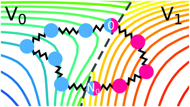 | ||
| Fig. 2 Illustration of a ring polymer on two diabatic PESs V0 and V1 in a two-dimensional nuclear configurational space. Only contours for the lowest PES are shown at any configuration. The blue (red) beads of the ring polymer represent the imaginary-time path on the reactant (product) electronic state. In this example, N0 = 6 and N1 = 4 giving a total of N = 10 beads. | ||
First we define Wolynes rate theory,65 which was derived via a second-order cumulant approximation of the time-correlation function66 and is given by
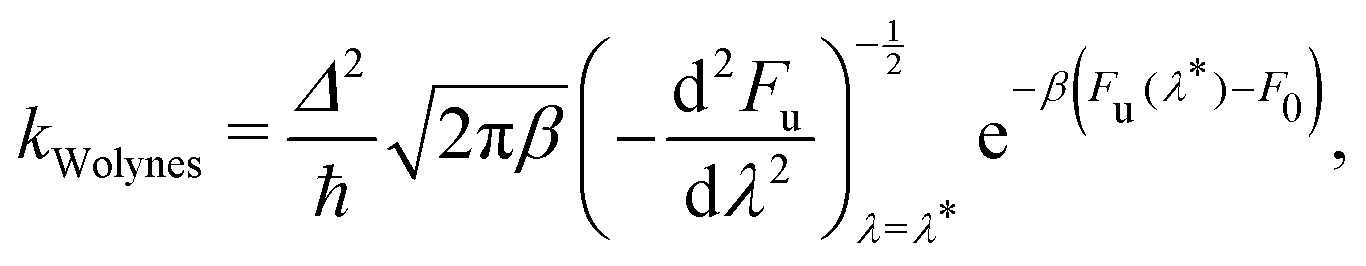 | (6) |
The GR-QTST method approximates the golden-rule rate using the ansatz:40
 | (7) |
 | (8) |
 . The virial energy estimators of the product and reactant paths, Ev0 and Ev0, are defined as in ref. 41 and are functions of the potentials and gradients of the beads corresponding to one particular state. The constraint is designed to enforce energy conservation for the ring polymers sampled in the simulation, which is known to give a strong connection to quantum transition-state theories.59
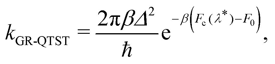
The classical rate in the golden-rule limit is defined by12,59
 | (9) |
 | (10) |
There are thus conceptual differences between Wolynes theory and GR-QTST. Wolynes theory relies on a steepest-decent approximation to the time integral of the flux–flux correlation function in the golden-rule limit,32 whereas GR-QTST incorporates the physical requirement of energy conservation enforced by the virial energy estimator.40 Both methods are approximations to the true quantum rate, but can be shown to be very accurate for simple systems such as the spin-boson model.40 It can also be shown that GR-QTST reduces to the classical rate, eqn (9), in the high-temperature limit of any system when the ring polymers collapse.40 However, the same is not necessarily true of Wolynes theory.59 In particular, we have shown that Wolynes theory can break down for systems with two or more different transition states, due to the fact that only one λ* value is used which cannot simultaneously be optimal for all transition states. In these cases at least, GR-QTST is expected to be more accurate as its rate is approximately independent of the choice of λ* and employs the energy constraint to ensure the correct sampling of each transition state.41
Computational methods
We computed rates from Wolynes theory and GR-QTST in the classical limit according to eqn (6) and (7). The free-energy term in the Wolynes rate was calculated using thermodynamic integration (TI) along the order parameter λ, | (11) |
 | (12) |
 | (13) |
The constrained free energy can then be expressed in terms of the sampling probability as
 | (14) |
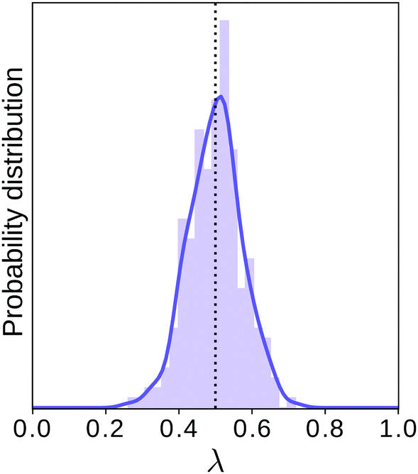
This procedure is computationally feasible if the unconstrained simulation samples enough configurations which obey the constraint  . If this condition is not fulfilled, the δ-TI method as described in ref. 41 could be applied in combination to calculate Fc(λ*). However, this was not necessary for the system studied in this work as can be seen from the histograms in both the classical and the quantum limit shown in Fig. 3, which are peaked around σ = 0.
 | ||
Fig. 3 Histograms of the values of  sampled in an unconstrained simulation and the corresponding kernel density estimation (KDE)67 in the classical and quantum limit. The KDE at σ = 0 is used to obtain the constrained free energy, Fc(λ*), used in the GR-QTST method. sampled in an unconstrained simulation and the corresponding kernel density estimation (KDE)67 in the classical and quantum limit. The KDE at σ = 0 is used to obtain the constrained free energy, Fc(λ*), used in the GR-QTST method. | ||
Due to this connection in methodology, one can use unconstrained PIMD simulations as a first step towards either Wolynes theory or GR-QTST rate calculations.
Both the Wolynes and GR-QTST rates can also be evaluated in the classical limit. The rate expressions kclWolynes and kclGR-QTST are very similar to eqn (6) and (7), with the only difference being that the employed free energies are replaced by their classical counterparts Fclu, Fclc and Fcl0. In the case of the classical Wolynes rate, the corresponding free-energy difference, Fclu − Fcl0, can be computed analogously to the quantum case (eqn (11)) with the ring polymer collapsed onto a single classical particle defined by the Hamiltonian
 | (15) |
Alternatively, Fclu − Fcl0 can be calculated by scaling up the mass of all the atoms (by multiplying mj by μ and taking the limit μ → ∞), which in effect collapses the ring polymer, making it behave classically.68–71 We found that both methods give results within each other's error bars for this system.
Note that kclWolynes is not the same as the classical rate expression in eqn (9), because Wolynes theory does not necessarily tend to the correct classical limit for general systems. However, when  is a linear function of λ (which is the case for spin-boson models), one can show that kclWolynes is the same as the rate of Marcus theory (eqn (2)), by plugging
 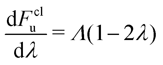 into eqn (6). In contrast, as we have shown in ref. 40, GR-QTST always reduces to the correct classical expression (eqn (9)) in the high-temperature limit where the ring polymer collapses. This gives us two other possible methods for calculating the classical rate, either by sampling the ensemble from the classical Hamiltonian
  to obtain Fclc following the same procedure given by eqn (14), or alternatively by scaling up the mass of all the atoms in a GR-QTST simulation.
In order to understand and to visualise the relation between all the different free energy terms in the rate theories introduced above, we constructed a thermodynamic cycle as shown in Fig. 4.
 | ||
| Fig. 4 Thermodynamic cycle containing all the free energy integration schemes of Wolynes theory and GR-QTST in the quantum and classical limit. Constrained free energies are obtained at a value of λ = λ*, which is the stationary point (SP) along the order parameter λ of the unconstrained free energy F(λ)u. | ||
The free-energy calculations necessary to compute Wolynes theory form the top and bottom horizontal thermodynamic paths of the left side of the cycle and relate the reactant (λ = 0) to the stationary point (λ = λ* = 0.5) in both the quantum and the classical limit. In order to compute GR-QTST, one additionally needs the free-energy calculations corresponding to the horizontal thermodynamic paths on the right side of the cycle. They can be viewed as an extension to the Wolynes free-energy calculations.
Each vertical thermodynamic path in the cycle represents a thermodynamic integration from the quantum nuclei to the classical limit using the mass-scaling factor μ as the order parameter (mass-TI).68–71 This means that each thermodynamic path of the cycle on the left can be calculated from independent simulations. Therefore, we use the left thermodynamic cycle to validate the accuracy and reliability of the free energies obtained from classical and quantum simulations, giving us further confidence in the Wolynes rates we computed. The free-energy differences, ΔF0 and ΔFu were calculated by performing two sets of PIMD simulations with H(λ)RP at λ = 0 and λ = λ*. The thermodynamic integrand was obtained for 10 different mass-scale factors from μ = 1 up to μ = 100. The contributions from larger μ values are also accounted for via a coordinate transform in the thermodynamic integration.69,70 We do not compute ΔFc as we found it to be numerically unstable to calculate due to the fact that the virial kinetic-energy estimator is not valid for constrained PIMD simulations. This free-energy change can however be inferred by completing the cycle.
The ion–ion distance was treated using a fixed-atom implementation at an interionic distance of r = 5.5 Å, which was determined to be the most probable interatomic distance for electron-transfer reactions.34,60 The interactions in the aqueous ferrous–ferric system are defined by the interatomic forces and pseudopotentials described in ref. 60 with the exception of the water model. In contrast to the formerly used rigid single point-charge (SPC) water model,34,60,72 we apply the flexible q-TIP4P/F water model,73 which was specifically developed to suit PIMD simulations. In particular, it can correctly capture the delicate balance between the competing quantum effects in water, compared to rigid or harmonic water models.73,74 Both, the q-TIP4P/F and SPC water models include electronic polarisation effects in a mean-field way75,76 and hence belong to the class of non-polarisable water models, which are computationally affordable and allow for extensive simulations. The application of an explicitly polarisable water model is crucial to describe effects in surface chemistry and clusters.77,78 The explicit treatment of polarisation is expected to lower the estimate of the reorganisation energy also in the aqueous ferrous–ferric system78–80 and it is therefore not without controversy to employ a non-polarisable water model. Ultimately, the choice of water model will of course affect the quantitative results, but will not hamper our ability to compare the different quantum rate theories. Nevertheless, it should be pointed out that several suggestions on polarisable water models and improved treatment of the solvent models were made in the literature.62,75–78,81
The reorganisation energy of the ferrous–ferric system calculated with the q-TIP4P/F water model is 108.5 ± 0.9 mHartree (68 kcal mol−1, 2.95 eV), which can be compared to the 128 mHartree (80 kcal mol−1, 3.5 eV) value found in the previous work34,60 using a rigid water model. Note that our setup gives a reorganisation energy only slightly closer to the experimental estimate of 2.1 eV.82
In order to obtain the rates for Wolynes theory and GR-QTST, we performed a set of PIMD simulations using N = 24 ring-polymer beads at 13 values of the order parameter λ (see eqn (3)) for each integral N0 value in the range N0 ∈ [0,12] to perform a thermodynamic integration along the order parameter λ. In each case, we averaged over 10 starting configurations picked randomly from a long MD simulation of the system with 265 water molecules in a cubic box of box length 20 Å (to give a water density of 103 kg m−3) using periodic boundary conditions. The temperature was set to 300 K and kept constant using the Andersen thermostat. Each simulation was then run under these conditions for 44![[thin space (1/6-em)]](https://www.rsc.org/images/entities/char_2009.gif) 000 steps (including 4000 steps of equilibration) with a timestep of 0.5 fs. The only additional information required to obtain a GR-QTST rate from such an unconstrained PIMD simulation is a histogram of the sampled values of the energy constraint function
000 steps (including 4000 steps of equilibration) with a timestep of 0.5 fs. The only additional information required to obtain a GR-QTST rate from such an unconstrained PIMD simulation is a histogram of the sampled values of the energy constraint function  . This has a very minor computational cost as it requires only one extra evaluation of the potential and forces on top of the N which are performed anyway at each step of the MD simulation. As we have chosen this setup in close analogy to the setup of ref. 60, the same considerations in terms of finite size effects and potential cutoffs apply. All of the classical MD forces are calculated using LAMMPS.83
Results and discussion
Our aim is to quantify the quantum effects present in the aqueous ferrous–ferric system and thereby to address the controversy of the magnitude of the effect of quantum tunnelling on the reaction rate. In this section we present results from both Wolynes theory and our newly developed GR-QTST40,41 and discuss the predictions for rate constants and isotope effects from these two different approaches. We investigate possible pitfalls of each theory and discuss how they affect the rate of this system. We then revisit the earlier studies34,60 to discover the effect of the improved water model and finally we compare our results with other quantum correction factors presented for the aqueous ferrous–ferric system in the literature.34 Underlying all the rate calculations are free-energy differences which were defined in the thermodynamic cycle introduced in Section 3. In Fig. 5 the results of these free-energy differences obtained from our simulations are given.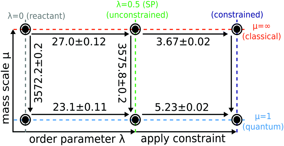 | ||
| Fig. 5 Thermodynamic cycle used to compute Wolynes theory and GR-QTST in the quantum and classical limit. Free energies are given in mHartree and error bars are of one standard deviation (1-sigma) calculated using block averaging84 and the error propagation formula. Cycle closure is observed for the unconstrained ensembles. The classical free energies were calculated using the mass-TI method. The classical Wolynes-theory calculation (thermodynamic integration along λ) performed using the collapsed ring-polymer method yields a free-energy change Fclu − Fcl0 = 27.1 ± 0.1 mHartree. | ||
Before comparing the results obtained from the two quantum rate theories, we first check for consistency of the calculations of the various free-energy paths presented in Fig. 5. Note that the Wolynes rate is defined in terms of the quantities belonging to the thermodynamic cycle on the left, whereas GR-QTST depends also on those on the right. As can be seen from Fig. 4, the free-energy change ΔΔFu is defined in two alternative ways
| ΔΔFu = (Fclu(λ*) − Fcl0) − (Fu(λ*) − F0) | (16a) |
| = ΔFu − ΔF0. | (16b) |
This free-energy change contributes exponentially to the quantum correction factor ΓWolynes introduced later (see Section 4.2, eqn (17)). It can thus be obtained either as a difference of a thermodynamic integration in the quantum and the classical limit as described in eqn (16a) and amounts to 3.9 ± 0.2 mHartree, or the difference between the mass-TI calculations at the reactant and stationary-point ensembles as defined in eqn (16b), which gives 3.6 ± 0.3 mHartree. The free-energy differences ΔF0 and ΔFu of eqn (16b) obtained from the different mass-TI calculations are significantly larger in magnitude, because they include the change from classical to quantum nuclei and therefore include the zero-point energy of the system. Further calculations are therefore made using the free energy differences as given by eqn (16a) in order to avoid the numerical errors inherent to a subtraction of large numbers. Nevertheless, the consistency (within error bars) of the free-energy difference ΔΔFu calculated via the two alternative routes also means that the left cycle is closed, which confirms that our Wolynes-theory simulations are converged.
Rates are then calculated according to eqn (6), (7) and (9) from the changes in free energy and are listed in Table 1 for both the classical limit (μ → ∞) and the quantum limit (μ = 1). It is interesting to note that the quantum rate predictions of GR-QTST and Wolynes theory do not agree. Both methods have been tested on the spin-boson model and give excellent and practically identical predictions of the quantum rate.40 However, due to the conceptual difference of the two theories, in more complex systems one cannot generally expect Wolynes theory and GR-QTST to predict similar rates. This therefore implies that the aqueous ferrous–ferric electron-transfer reaction is fundamentally more complex than the spin-boson model. A second obvious conclusion is that since the two theories do not agree, at least one rate prediction must be inaccurate. In the following we analyse the two methods to discuss these points.
| Rate | Classical | Quantum (H2O) | Quantum (D2O) |
|---|---|---|---|
| k Marcus | 7.0 ± 1.7 × 10⁻¹¹ | — | — |
| k cl | 7.3 ± 1.0 × 10⁻¹¹ | — | — |
| k Wolynes | 7.6 ± 1.0 × 10⁻¹¹ | 5.3 ± 0.7 × 10⁻⁹ | 2.7 ± 0.3 × 10⁻⁹ |
| k GR-QTST | 6.3 ± 0.9 × 10⁻¹¹ | 7.6 ± 0.9 × 10⁻¹⁰ | 4.5 ± 0.4 × 10⁻¹⁰ |
Making or breaking of Wolynes theory
As presented in ref. 41, a break-down of Wolynes theory occurs when the system under investigation exhibits multiple distinct transition states, which can lead to an overprediction of the rate by orders of magnitude. There are a number of criteria that serve as indicators to identify whether Wolynes theory is applicable, although the absence of these features does not exclude the possibility of at least a minor break down of Wolynes theory. The first criterion is whether the rate tends to the correct classical limit as the masses are scaled up. Second, one should investigate the ensemble of paths sampled by the unconstrained simulation to check that these are centred around energy-conserving paths like the instantons. Finally, any evidence for the existence of multiple transition states with a range of different λ values would suggest that Wolynes theory is not valid as it cannot simultaneously satisfy the condition for each transition state.In the classical (high-temperature or heavy mass) limit, in contrast to Wolynes theory, GR-QTST is known to tend to the correct classical rate,40 and our simulations are in agreement with this (see Table 1). As suggested above, there is no rigorous argument that requires Wolynes theory to correctly predict the true classical rate and this thus provides a good check that the method gives physically sensible results. In this case, it does give the correct result within the error bars. This success of Wolynes theory in the classical limit can be related to the approximately linear behaviour of the free-energy derivative with respect to the order parameter, λ, as shown in Fig. 6. This is a clear indication that the linear-response approximation is valid for this system in the classical limit, as was already discussed in previous work.12,60,62 As a consequence, the classical limit of the aqueous ferrous–ferric system strongly resembles a spin-boson model, where Wolynes theory is known to perform well. The same also explains the good agreement of Marcus theory with the exact classical rate, because Marcus theory, similarly to Wolynes theory, is known to perform well for this model. For a quantitative comparison, we note that the free-energy barrier according to Marcus theory is Λ/4 = 27.1 mHartree, which is in excellent agreement with that found from Wolynes theory in the classical limit (27.0 ± 0.12 mHartree). Note that this is not always the case for asymmetric reactions, where the linear-response approximation is commonly seen to break down.85
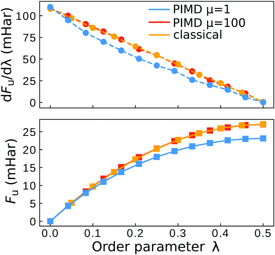 | ||
| Fig. 6 Plot of the Wolynes free energy derivative and free energy. The “classical” result refers to the simulation with a collapsed ring polymer (eqn (15)). The error bars are smaller than the symbol size. | ||
The aqueous ferrous–ferric system therefore does not exhibit a break-down of Wolynes theory in the classical limit, in contrast to the model systems tested in ref. 41.
The investigation of the second qualitative indicator of break-down of Wolynes theory is the distribution of values of  which are sampled in the unconstrained ensemble. If this distribution had a negligible population at σ = 0, which was the case for the system under study in ref. 41, it would imply that the paths being sampled have no connection to the energy-conserving instantons and would be a clear sign of the break-down of Wolynes theory. However, as shown in Fig. 3, Wolynes-theory calculations sample a uni-modal distribution peaked around σ = 0. This therefore neither confirms nor disproves a break-down of Wolynes theory in this system.
A more detailed observation can be made from a comparison to another quantum rate theory, namely instanton theory. Instanton theory is not rigorously applicable to reactions in solution26 and we cannot therefore use it to calculate the rate. However, we can nonetheless acquire a qualitative insight into the tunnelling pathways of the system by obtaining a set of optimised instanton paths28 on different solvent configurations randomly taken from a MD simulation (250 configurations). All instanton optimisations were able to find non-trivial tunnelling pathways, which suggests that nuclear tunnelling is a significant contributor to the quantum rate enhancement. The water molecules beyond a radius of 5 Å of either Fe ion were fixed and only water molecules within this circumference were optimised in the instanton calculations (approximately 36 flexible water molecules). Analysing the ensemble of instantons clearly shows that the aqueous ferrous–ferric system has multiple transition states. As shown in Fig. 7, the instantons have a range of different order parameters λ, which are found by a stationary-action principle.24 A distribution of instantons occurs because even though the system is globally symmetric, it is locally asymmetric around each instanton and this is another sign that the system differs from the spin-boson model, which has only one instanton with λ = 0.5. The order parameters for each instanton cannot all be simultaneously satisfied by the single choice made by Wolynes theory of λ* = 0.5, which suggests that Wolynes theory may break down for this system and overpredict the rate in the quantum limit. However, a broad uni-modal distribution as observed here is clearly a much safer scenario for Wolynes theory than the system tested in ref. 41 for which this equivalent plot would have two peaks on either side of λ*. The fact that in this case the distribution is uni-modal and centred at λ = 0.5 (with a standard deviation of 0.07) suggests that the break down will be less severe.
 | ||
| Fig. 7 Distribution of the λ values found from the ensemble of instantons. The dotted line shows λ* = 0.5, which is the value appropriate for Wolynes theory, and due to symmetry is also the average of the ensemble of instantons. | ||
Discussion of the GR-QTST result
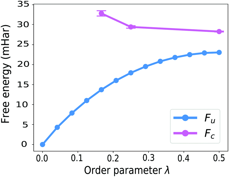
GR-QTST, in contrast to Wolynes theory, can treat systems with multiple transition states correctly,41 and similarly to Wolynes theory, gives an accurate result for the spin-boson model in both the classical and the quantum limit.40 In fact, the close agreement of GR-QTST and Wolynes theory for a spin-boson model40 is another argument towards the aqueous ferrous–ferric system being badly approximated by a spin-boson model in the quantum limit, because for this system the two rate theories disagree (see Table 1).Next to the discrepancy in rates, the curvature of the constrained free energy Fc(λ) shown in Fig. 8 can be utilised to argue against the applicability of linear-response theory and therefore the approximation of this system by a spin-boson model. Unlike the observation for a spin-boson model, for the atomistic system under study the constrained free energy Fc(λ) is curved upwards in extreme regions of the order parameter λ, i.e. far from the optimal order parameter λ*. In the earlier investigation of GR-QTST on spin-boson models,40 we found that the constrained free energy Fc(λ) curves down when going away from the optimal order parameter λ*. This curvature behaviour becomes more prominent with an increased number of degrees of freedom and is already significant for 8 degrees of freedom, which can be understood based on the analysis presented in ref. 40. The fact that the curvature behaviour differs from this is a further indicator for the aqueous ferrous–ferric system not being well described by a spin-boson model.
 | ||
| Fig. 8 Comparison of the curvature of the free energies of Wolynes (unconstrained) and GR-QTST (constrained) along the path-splitting parameter λ. We obtained the constrained free energies Fc(λ) at values of λ ≠ 0.5 by combination of the δ-TI method and histogramming. The error bars on the unconstrained calculations are smaller than the marker size. | ||
The curvature of the constrained free energy Fc(λ) is also of interest as it is an indication of the size-consistency error of GR-QTST. In ref. 40 we showed that as more degrees of freedom are added to the system, the plot of Fc(λ) becomes more and more curved. However, we also argued that no matter how large the system, it becomes flat in the classical limit, and that for a spin-boson model, the value of Fc(λ*) remains stable even in the quantum case. There is however the possibility that this could lead to an error for more complex systems such as the aqueous ferrous–ferric reaction studied here. However, in the broad vicinity of the stationary point λ* the curvature of the constraint free energy is approximately flat. This is a good sign that there is no serious error being made by the GR-QTST method.
New and old controversies of the aqueous ferrous–ferric electron transfer
Of particular interest is the enhancement of the electron-transfer rate due to nuclear quantum effects, which can be quantified by the quantum correction factor Γ, defined as the ratio of the quantum and the classical rate. Already 30 years ago the investigation of the aqueous ferrous–ferric system led to a broad range of predictions for this quantity,34,62,63 and no conclusive argument could be made at the time for which was correct. We reopen this controversy by adding the results of our new GR-QTST approach to the discussion.We define Γ for each quantum rate theory, for example
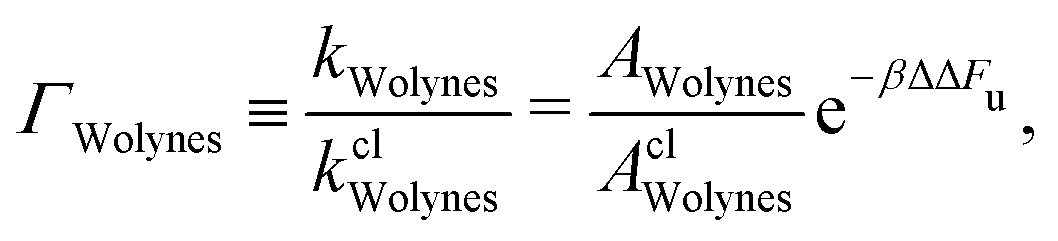 | (17) |
The prefactor ratio AWolynes/AclWolynes is generally not exactly equal to 1, although the equivalent term for GR-QTST is identically 1 and does not therefore appear. Accordingly, the quantum correction factor for GR-QTST can be defined simply as ΓGR-QTST = e−βΔΔFc with the exponent
| ΔΔFc = (Fc(λ*) − F0) − (Fclc(λ*) − Fcl0). | (18) |
Defining the quantum correction factor in this way gives the most fair comparison between methods as it would allow for some error cancellation in the case that Wolynes theory breaks down and overestimates the rate in both the classical and quantum limit. Γ therefore describes the quantum rate enhancement described by a given theory and avoids inconsistencies by cross-comparison of different theories.
The quantum correction factor gives a measure of nuclear tunnelling in the reaction. Note that it is tricky to rigorously separate the tunnelling contribution from other NQEs such as vibrational quantisation86 and it therefore technically quantifies the rate enhancement from all NQEs. In the case of the spin-boson model, however, the potentials are harmonic which ensures that zero-point energy is the same everywhere. Tunnelling is thus the only factor contributing to the quantum rate enhancement in this case.34 Although this argument does not hold rigorously for the atomistic system, we assume that nuclear tunnelling continues to play an important role in this system and present evidence in the ESI† to support this based on the instanton optimisations described above.
The quantum correction factors obtained from various rate theories are reported in Table 2. Our results from Wolynes theory are in agreement with similar calculations performed by Chandler and co-workers34 despite the fact that we employed a different water model. This appears to be a bit of a coincidence because when we map our system (with the flexible q-TIP4P/F water) on to a spin-boson model following the same procedure as in ref. 34 (for which the spectrum is shown in the ESI†) and solve for the exact quantum rate,39 we find a large quantum correction factor of Γspin-boson = 83. This is more than a factor of two larger than the tunnelling enhancement (Γspin-boson = 36) found for the SPC water model.34 In part this deviation can be attributed to the contribution of high-frequency modes (H-bond bending and stretching) of the flexible water model. Integration of the spectral density gives a reorganisation energy of 3.1 ± 0.2 eV, in which 90% comes from the low frequency modes. It is, however, due to the NQEs of the high-frequency modes that we obtain a larger quantum correction factor,79Γspin-boson, with q-TIP4P/F water, as can be shown from the fact that if we only accounted for the low-frequency modes, we would predict that Γspin-boson was only 15. The reason that Γspin-boson = 36 for SPC water is not as low as this is a result of its overall larger reorganisation energy (Λ = 3.5 eV). In order to show this we used the low-frequency part of the q-TIP4P/F spectral density and scaled it up to produce Λ = 3.5 eV. In this case Γspin-boson increases to 28, which is closer to the result of SPC water. This analysis shows that the two water models are significantly different. It so happens that, due to the two competing effects of flexibility and the lower reorganisation energy of the q-TIP4P/F model, we obtain similar a result within Wolynes theory, but a different result for the spin-boson model.
| This work | Ref. 34 | |
|---|---|---|
| Γ Wolynes | 70 ± 13 | 65 ± 6 |
| Γ GR-QTST | 12 ± 2 | — |
| Γ spin-boson | 83 | 36 |
It also appears to be a coincidence that the quantum correction factor predicted by Wolynes theory using the flexible q-TIP4P/F and the spin-boson model give such similar results. We have presented a number of arguments throughout this paper to explain why one would not in general expect them to be the same, and indeed this was not found to be the case in the study by Chandler and co-workers.34 The most important finding of this work is that the predictions from Wolynes theory and GR-QTST differ significantly. Each of the three methods presented in Table 2 employs a different approximation and it is difficult to determine which (if any) is correct as no exact quantum-mechanical rate for the aqueous ferrous–ferric system can be computed. A comparison to experimental results is, however, another possible aspect to investigate.
For the ferrous–ferric system experimental isotope effects are available and the presence of a kinetic isotope effect is proof that NQEs play a role in this reaction as the classical rate does not depend on the masses of the atoms. The experimental estimate of the isotope effect is in the range of kHexp/kDexp = 1.7–2.0,87,88 which compares well to the ratio kHWolynes/kDWolynes = 2.0 ± 0.4 that we find by employing Wolynes rate theory for both isotopes. Our Wolynes-theory calculations show an increase of the free energy difference from (Fu − F0)H = 23.1 ± 0.11 mHartree for the hydrogen isotope to (Fu − F0)D = 23.8 ± 0.12 mHartree for the deuterium isotope. Our prediction of the isotope effect from the GR-QTST calculations is kHGR-QTST/kDGR-QTST = 1.7 ± 0.3 and thus also lies within the range of experimental findings. The GR-QTST prediction is slightly lower than that of Wolynes theory, because nuclear tunnelling plays a smaller role (see Table 2). Ref. 34 reported an isotope factor of kHWolynes/kDWolynes = 2.6 ± 0.5.
Although our main focus is on the comparison of different quantum rate theories, in order to justify our comparison with the experimental isotope effect, we must also consider the accuracy of the atomistic model. As we have already discussed earlier the choice of the water model has a crucial effect on the predicted rates and NQEs. Marcus and co-workers62 predict a significantly lower quantum correction factor of Γspin-boson = 9.6 (using the spin-boson model63 with an experimental spectral density) than Chandler and co-workers’ results. Note that this result cannot be taken as a benchmark as it is based on the spin-boson model, which we argue is a questionable approximation. They proposed in ref. 62 that the discrepancy in the two predictions might be due to the neglect of electronic polarisation and flexibility of water in ref. 34, although as they are competing effects they may cancel to a certain extent.78 We have explicitly included the flexibility of water molecules in our study and found that it can have a significant impact on the rate enhancement due to nuclear tunnelling. Nonetheless, although we predict a lower reorganisation energy (2.95 eV) using the flexible water model than Chandler and co-workers (3.5 eV)34 do with the rigid one, neither water model reproduces the experimentally estimated reorganisation energy (2.1 eV).82 If we were to include electronic polarisation as well, one would expect the reorganisation energy to decrease. This is turn could result in reduced tunnelling effects.78
This work therefore aims to reopen the discussion on the question of tunnelling enhancement in the atomistic model of the ferrous–ferric electron transfer as presented here. The majority of previous studies on this question have concentrated on exploring the effect of changing the spectral density of the bath62 or improving the description of the atomistic model.79 We have, however, explored how the predictions depend on the choice of quantum rate theory used for a given system Hamiltonian. We have shown that a number of different methods obtain different rate predictions and currently no decisive argument for which (if any) gives the correct result can be made. This is reminiscent of the controversy surrounding the quantum tunnelling effect in the Azzouz-Borgis model of proton transfer, for which various approximate quantum rate theories do not agree.50,89–91 Any further study of these problems however provides valuable insights into the accuracy, applicability and pitfalls of the quantum methods applied.
Conclusions
In this study, we have presented the first application of GR-QTST to an atomistic system of electron transfer and thereby obtained estimates for the reaction rate, isotope and tunnelling enhancement effects from this new method. The aqueous ferrous–ferric electron-transfer reaction has been extensively studied in the past and yet no conclusive quantitative answer for the contribution of nuclear tunnelling to the reaction rate has been given. In fact the previously predicted quantum correction factors span an order of magnitude34,60,62,63 and our new prediction is at the lower end of this range.All the methods tested reproduce the correct rate in the classical limit. GR-QTST is guaranteed to do this for any system, whereas Wolynes theory and Marcus theory are correct only if the linear-response approximation is valid. This implies that the classical limit of this reaction can be adequately described by a spin-boson model. This observation may lead one to believe that the spin-boson model is a valid approximation of the aqueous ferrous–ferric system also in the quantum limit. However, we could show the unsuitability of this assumption by comparing Wolynes theory32 and our newly developed GR-QTST.40,41 In an earlier study it was observed that GR-QTST and Wolynes theory predict the same rate for a spin-boson model in the quantum limit.40 In contrast to this, the two theories predict quantum correction factors that differ by a factor of 6 for the atomistic system, therefore making it impossible to argue that a spin-boson model is a good approximation in this case.
The obvious next question aims at resolving the disagreement of Wolynes theory and GR-QTST and in order to do so the possible pitfalls of each method were investigated. We have explained that there is a risk that Wolynes theory may break down and overpredict the rate, especially in liquid systems like that under study. This may occur whenever a reaction contains multiple distinct transition states.41 We optimised a set of instantons in the system and found that their order parameters, λ, were distributed around λ* = 0.5. This implies that there are indeed multiple transition states in this system, although they are more similar to each other than the extreme cases studied in ref. 41. The error made by Wolynes theory is thus expected to be less severe, but may still exist to some extent. GR-QTST is also not without its flaws and we have shown in previous work that the theory may suffer from size inconsistency. In a model system the addition of many degrees of freedom leads to a strongly λ-dependent Fc(λ) curve, which may degrade the rate predictions. Nevertheless, for the high-dimensional aqueous ferrous–ferric system, we observe only a minor curving of the constrained free energy of GR-QTST far from the optimal order parameter λ*, which is not expected to significantly degrade the result.
Considering the discrepancy in the predicted tunnelling enhancement makes it however apparent that at least one theory must be inaccurate for this system. A hypothesis that Wolynes theory is overpredicting the rate due to the multi-instanton nature of the system cannot be excluded from the results of our calculations. However, none of the studies provide us with a conclusive case to prove this statement, nor to rule out the possibility of an error on the part of GR-QTST. By revisiting the controversial question of the nuclear tunnelling effect in this system, we could however show that the dynamics in this system deviates from those of the spin-boson model and raises the question of the applicability of this model for simulating atomistic systems. We hope to further elucidate the question of appropriateness of these quantum rate theories, by applying GR-QTST to a more complex atomistic system, where Wolynes theory may show more distinctive break-down behaviour.
Conflicts of interest
There are no conflicts to declare.Acknowledgements
We thank Manish J. Thapa, Joseph E. Lawrence and Prof. Jochen Blumberger for the helpful discussions. The authors acknowledge financial support from the Swiss National Science Foundation through Project 175696.Notes and references
- R. P. Bell, The Tunnel Effect in Chemistry, Chapman and Hall, London, 1980 Search PubMed.
- S. T. Bromley, T. P. M. Goumans, E. Herbst, A. P. Jones and B. Slater, Phys. Chem. Chem. Phys., 2014, 16, 18623–18643 RSC.
- V. Singh, D. Atta, M. Khan and D. Basu, Nuc. Phys. A, 2019, 986, 98–106 CrossRef CAS.
- B. K. Carpenter, J. Am. Chem. Soc., 1983, 105, 1700–1701 CrossRef CAS.
- R. J. McMahon, Science, 2003, 299, 833–834 CrossRef CAS PubMed.
- D. D. Vault and B. Chance, Biophys. J., 1966, 6, 825–847 CrossRef.
- A. Warshel and R. P. Bora, J. Chem. Phys., 2016, 144, 180901 CrossRef PubMed.
- S. C. L. Kamerlin, J. Mavri and A. Warshel, FEBS Lett., 2010, 584, 2759–2766 CrossRef CAS PubMed.
- R. A. Marcus, Annu. Rev. Phys. Chem., 1964, 15, 155–196 CrossRef CAS.
- R. A. Marcus and N. Sutin, Biochim. Biophys. Acta, 1985, 811, 265–322 CrossRef CAS.
- R. A. Marcus, Rev. Mod. Phys., 1993, 65, 599–610 CrossRef CAS.
- D. Chandler, in Classical and Quantum Dynamics in Condensed Phase Simulations, ed. B. J. Berne, G. Ciccotti and D. F. Coker, World Scientific, Singapore, 1998, ch. 2, pp. 25–49 Search PubMed.
- E. Fermi, Nuclear Physics, University of Chicago Press, Chicago, 1974 Search PubMed.
- A. Nitzan, Chemical Dynamics in Condensed Phases: Relaxation, Transfer, and Reactions in Condensed Molecular Systems, Oxford University Press, Oxford, 2006 Search PubMed.
- J. E. Lawrence and D. E. Manolopoulos, Faraday Discuss., 2020, 221, 9–29 RSC.
- R. P. Feynman and A. R. Hibbs, Quantum Mechanics and Path Integrals, McGraw-Hill, New York, 1965 Search PubMed.
- T. E. Markland and M. Ceriotti, Nat. Rev. Chem., 2018, 2, 0109 CrossRef CAS.
- D. Chandler and P. G. Wolynes, J. Chem. Phys., 1981, 74, 4078–4095 CrossRef CAS.
- W. H. Miller, J. Phys. Chem. A, 1998, 102, 793–806 CrossRef CAS.
- A. A. Kananenka, X. Sun, A. Schubert, B. D. Dunietz and E. Geva, J. Chem. Phys., 2018, 148, 102304 CrossRef PubMed.
- N. Makri, Int. J. Quantum Chem., 2015, 115, 1209–1214 CrossRef CAS.
- W. H. Miller, J. Chem. Phys., 1975, 62, 1899–1906 CrossRef CAS.
- S. Coleman, Proc. Int. School of Subnuclear Physics, Erice, 1977.
- J. O. Richardson, J. Chem. Phys., 2018, 148, 200901 CrossRef PubMed.
- J. O. Richardson, J. Chem. Phys., 2016, 144, 114106 CrossRef PubMed.
- J. O. Richardson, Int. Rev. Phys. Chem., 2018, 37, 171–216 Search PubMed.
- J. O. Richardson, R. Bauer and M. Thoss, J. Chem. Phys., 2015, 143, 134115 CrossRef PubMed.
- J. O. Richardson, J. Chem. Phys., 2015, 143, 134116 CrossRef PubMed.
- J. Mattiat and J. O. Richardson, J. Chem. Phys., 2018, 148, 102311 CrossRef PubMed.
- E. R. Heller and J. O. Richardson, J. Chem. Phys., 2020, 152, 034106 CrossRef PubMed.
- J. B. Rommel, Y. Liu, H.-J. Werner and J. Kästner, J. Phys. Chem. B, 2012, 116, 13682–13689 CrossRef CAS PubMed.
- P. G. Wolynes, J. Chem. Phys., 1987, 87, 6559–6561 CrossRef.
- M. Parrinello and A. Rahman, J. Chem. Phys., 1984, 80, 860–867 CrossRef CAS.
- J. S. Bader, R. A. Kuharski and D. Chandler, J. Chem. Phys., 1990, 93, 230–236 CrossRef CAS.
- C. Zheng, J. A. McCammon and P. G. Wolynes, Proc. Natl. Acad. Sci. U. S. A., 1989, 86, 6441–6444 CrossRef CAS PubMed.
- C. Zheng, J. A. McCammon and P. G. Wolynes, Chem. Phys., 1991, 158, 261–270 CrossRef CAS.
- J. E. Lawrence and D. E. Manolopoulos, J. Chem. Phys., 2018, 148, 102313 CrossRef PubMed.
- J. Cao and G. A. Voth, J. Chem. Phys., 1997, 106, 1769 CrossRef CAS.
- U. Weiss, Quantum Dissipative Systems, World Scientific, Singapore, 4th edn, 2012 Search PubMed.
- M. J. Thapa, W. Fang and J. O. Richardson, J. Chem. Phys., 2019, 150, 104107 CrossRef PubMed.
- W. Fang, M. J. Thapa and J. O. Richardson, J. Chem. Phys., 2019, 151, 214101 CrossRef PubMed.
- W. H. Miller, Y. Zhao, M. Ceotto and S. Yang, J. Chem. Phys., 2003, 119, 1329–1342 CrossRef CAS.
- C. L. Vaillant, M. J. Thapa, J. Vaníček and J. O. Richardson, J. Chem. Phys., 2019, 151, 144111 CrossRef PubMed.
- I. R. Craig and D. E. Manolopoulos, J. Chem. Phys., 2004, 121, 3368–3373 CrossRef CAS PubMed.
- I. R. Craig and D. E. Manolopoulos, J. Chem. Phys., 2005, 122, 084106 CrossRef PubMed.
- I. R. Craig and D. E. Manolopoulos, J. Chem. Phys., 2005, 123, 034102 CrossRef PubMed.
- J. O. Richardson and S. C. Althorpe, J. Chem. Phys., 2009, 131, 214106 CrossRef PubMed.
- S. Habershon, D. E. Manolopoulos, T. E. Markland and T. F. Miller III, Annu. Rev. Phys. Chem., 2013, 64, 387–413 CrossRef CAS PubMed.
- N. Boekelheide, R. Salomón-Ferrer and T. F. Miller III, Proc. Natl. Acad. Sci. U. S. A., 2011, 108, 16159–16163 CrossRef CAS PubMed.
- R. Collepardo-Guevara, I. R. Craig and D. E. Manolopoulos, J. Chem. Phys., 2008, 128, 144502 CrossRef PubMed.
- A. R. Menzeleev, N. Ananth and T. F. Miller, III, J. Chem. Phys., 2011, 135, 074106 CrossRef PubMed.
- A. R. Menzeleev, F. Bell and T. F. Miller III, J. Chem. Phys., 2014, 140, 064103 CrossRef PubMed.
- J. S. Kretchmer and T. F. Miller III, Faraday Discuss., 2016, 195, 191–214 RSC.
- J. S. Kretchmer, N. Boekelheide, J. J. Warren, J. R. Winkler, H. B. Gray and T. F. Miller III, Proc. Natl. Acad. Sci. U. S. A., 2018, 115, 6129–6134 CrossRef CAS PubMed.
- X. Tao, P. Shushkov and T. F. Miller III, J. Chem. Phys., 2018, 148, 102327 CrossRef PubMed.
- X. Tao, P. Shushkov and T. F. Miller III, J. Phys. Chem. A, 2019, 123, 3013–3020 CrossRef CAS PubMed.
- J. E. Lawrence, T. Fletcher, L. P. Lindoy and D. E. Manolopoulos, J. Chem. Phys., 2019, 151, 114119 CrossRef PubMed.
- J. E. Lawrence and D. E. Manolopoulos, J. Chem. Phys., 2019, 151, 244109 CrossRef PubMed.
- J. O. Richardson and M. Thoss, J. Chem. Phys., 2014, 141, 074106 CrossRef PubMed.
- R. A. Kuharski, J. S. Bader, D. Chandler, M. Sprik, M. L. Klein and R. W. Impey, J. Chem. Phys., 1988, 89, 3248–3257 CrossRef CAS.
- M. Marchi and D. Chandler, J. Chem. Phys., 1991, 95, 889 CrossRef CAS.
- X. Song and R. A. Marcus, J. Chem. Phys., 1993, 99, 7768–7773 CrossRef CAS.
- P. Siders and R. A. Marcus, J. Am. Chem. Soc., 1981, 103, 741–747 CrossRef CAS.
- M. Bixon and J. Jortner, Adv. Chem. Phys., 1999, 106, 35–202 CAS.
- P. G. Wolynes, J. Chem. Phys., 1987, 87, 6559–6561 CrossRef.
- W. H. Miller, S. D. Schwartz and J. W. Tromp, J. Chem. Phys., 1983, 79, 4889–4898 CrossRef CAS.
- D. W. Scott, Multivariate Density Estimation: Theory, Practice, and Visualization, John Wiley & Sons, New York, 1992 Search PubMed.
- A. Pérez and O. A. von Lilienfeld, J. Chem. Theory Comput., 2011, 7, 2358–2369 CrossRef PubMed.
- M. Ceriotti and T. E. Markland, J. Chem. Phys., 2013, 138, 014112 CrossRef PubMed.
- W. Fang, J. Chen, M. Rossi, Y. Feng, X.-Z. Li and A. Michaelides, J. Phys. Chem. Lett., 2016, 7, 2125–2131 CrossRef CAS PubMed.
- V. Kapil, E. Engel, M. Rossi and M. Ceriotti, J. Chem. Theory Comput., 2019, 15, 5845–5857 CrossRef CAS PubMed.
- H. J. C. Berendsen, J. P. M. Postma, W. F. van Gunsteren and J. Hermans, in Intermolecular Forces, ed. B. Pullman, Reidel, Dordrecht, 1981 Search PubMed.
- S. Habershon, T. E. Markland and D. E. Manolopoulos, J. Chem. Phys., 2009, 131, 024501 CrossRef PubMed.
- M. Ceriotti, W. Fang, P. G. Kusalik, R. H. McKenzie, A. Michaelides, M. A. Morales and T. E. Markland, Chem. Rev., 2016, 116, 7529–7550 CrossRef CAS PubMed.
- H. J. C. Berendsen, J. R. Grigera and T. P. Straatsma, J. Phys. Chem., 1987, 91, 6269–6271 CrossRef CAS.
- K. Watanabe and M. L. Klein, Chem. Phys., 1989, 131, 157–167 CrossRef CAS.
- T.-M. Chang and L. X. Dang, Chem. Rev., 2006, 106, 1305–1322 CrossRef CAS PubMed.
- J. Blumberger, Phys. Chem. Chem. Phys., 2008, 10, 5651–5667 RSC.
- J. Blumberger and G. Lamoureux, Mol. Phys., 2008, 106, 1597–1611 CrossRef CAS.
- P. Ren and J. W. Ponder, J. Phys. Chem. B, 2003, 107, 5933–5947 CrossRef CAS.
- J. Blumberger and M. Sprik, Theor. Chem. Acc., 2006, 115, 113–126 Search PubMed.
- K. M. Rosso and J. R. Rustad, J. Phys. Chem. A, 2000, 104, 6718–6725 CrossRef CAS.
- S. Plimpton, J. Comput. Phys., 1995, 117, 1–19 CrossRef CAS.
- M. P. Allen and D. J. Tildesley, Computer Simulation of Liquids, Clarendon Press, New York, 1989 Search PubMed.
- J. Blumberger, I. Tavernelli, M. L. Klein and M. Sprik, J. Chem. Phys., 2006, 124, 064507 CrossRef PubMed.
- G. C. Schatz, Chem. Rev., 1987, 87, 81–89 CrossRef CAS.
- J. Hudis and R. W. Dodson, J. Am. Chem. Soc., 1956, 78, 911–913 CrossRef CAS.
- T. Guarr, E. Buhks and G. McLendon, J. Am. Chem. Soc., 1983, 105, 3763–3767 CrossRef CAS.
- S. Hammes-Schiffer and J. C. Tully, J. Chem. Phys., 1994, 101, 4657–4667 CrossRef CAS.
- I. R. Craig, M. Thoss and H. Wang, J. Chem. Phys., 2011, 135, 064504 CrossRef PubMed.
- K. Karandashev, Z.-H. Xu, M. Meuwly, J. Vaníček and J. O. Richardson, Struct. Dyn., 2017, 4, 061501 CrossRef PubMed.
Footnotes |
| † Electronic supplementary information (ESI) available. See DOI: 10.1039/c9cp06841d |
| ‡ These authors contributed equally. |
| This journal is © the Owner Societies 2020 |