Early warning signals in chemical reaction networks

Abstract

Complex systems such as ecosystems, the climate and stock markets produce emergent behaviour which is capable of undergoing dramatic change when pushed beyond a tipping point. Such complex systems display Early Warning Signals in their behaviour when they are close to a tipping point. Here we show that a complex chemical reaction network can also display early warning signals when it is in close proximity to the boundary between oscillatory and steady state concentration behaviours. We identify early warning signals using both an active sensing method, based on the recovery time of an oscillatory response after a perturbation in temperature, and a passive sensing method, based upon a change in the shape of the oscillations. The presence of the early warning signals indicates that complex, dissipative chemical networks can intrinsically sense their proximity to a boundary between behaviours.

---

The natural world and human societies are complex systems whereby the interactions of many different actors with each other and with their environment produce emergent behaviour (e.g. population dynamics, shifts in climate, brain waves and movements in financial markets).¹ Complex systems can be subject to dramatic changes in behaviour, e.g. ecosystem collapse, brain seizures and financial crashes, when the system is pushed beyond a so-called tipping point.^2–4 A tipping point occurs at a boundary between two characteristically different behaviours that can emerge from the system. Analysis of complex systems by ecologists, climatologists, neuroscientists^5,6 and economists⁷ have revealed that when a system is held in close proximity to a tipping point certain characteristic ‘early warning signals’ are produced by the system. Early warning signals include critical slowing down behaviour, where after a small perturbation the system takes longer to recover to its original state when it is near the boundary between behaviours than when it is far from it.⁹ Another example of an early warning signal are changes in spatial patterns close to a tipping point, foreshadowing a collapse transition.^3,10,11 The reading of early warning signals can highlight when corrective actions need to be taken in order to return the system to a more stable state.

Early warning signals may also enable the detection of the boundaries of the ‘functional regimes’ in chemical reaction networks. The design of complex chemical reaction networks capable of producing emergent behaviour has become of increasing interest to chemists and has led to development of the field of systems chemistry.¹² The aim of which is to design chemical systems capable of producing life-like behaviour, and examples include systems designed to oscillate,^8,13–17 multiple oscillator systems that synchronise via diffusional spatiotemporal coupling,¹⁸ bistable systems,¹⁹ wave fronts,^20,21 chemically fuelled transiently formed micelles²² and adaptive response networks.²³ Whether the behaviour of such designed chemical systems are capable of indicating through early warning signals their proximity to a boundary change in behaviour remains unknown.

We sought to ascertain whether a minimal chemical reaction network produces early warning signals as these could play an important role in the future design and function of out-of-equilibrium systems. To do this we took our previously reported trypsin oscillator system (Fig. 1b) that produces two possible behaviours in flow (i) sustained oscillations in the concentration of the enzyme trypsin (Fig. 1a left), or, (ii) dampened oscillations leading to a steady state concentration of trypsin (Fig. 1a right).⁸ Which behaviour is produced depends upon the concentrations of reagents used and upon the conditions of the environment, namely temperature and flow rate.²⁴ Within the temperature range 15–38 °C and flow rates 0.05–0.8 h⁻¹ the system produces sustained oscillations in trypsin concentration. Outside of this optimum range the system produces dampened oscillations that lead to a steady state concentration.

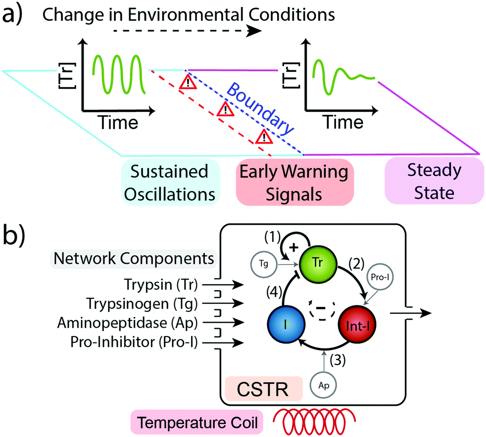Fig. 1 (a) Our network can generate two possible behaviours: sustained oscillations in the concentration of trypsin (left) and dampened oscillations to a steady state concentration of trypsin (right). If a change in environmental conditions pushes the system over the boundary then the behaviour of the system will change. As changes in the environment bring the system closer to the boundary it will begin to display Early Warning Signals indicating its proximity to the boundary and to an alteration in its behaviour. (b) Schematic representation of the Trypsin oscillator. The network consists of four main processes; (1) Trypsinogen (Tg) autocatalysis and (2) pro-inhibitor (Pro-I) activation, both catalysed by Tr, (3) delayed inhibitor activation from an intermediate inhibitor (Int-I) catalysed by aminopeptidase (Ap), and (4) Tr inhibition by inhibitor (I).⁸ The network is kept out-of-equilibrium in a Continuous Stirred Flow Tank Reactor (CSTR).

We set out to see if the system gave any early warning signals through its behaviour when it was operated close to the boundary between its two behaviours. We explore both (i) an ‘active’ sensing method whereby we make an intervention to the system, observe its response and then follow how this response varies in relation to the systems proximity to the boundary, and, (ii) a ‘passive’ sensing method whereby we make no intervention and only observe changes in the behaviour of the system as it is brought close to the boundary.

The ‘active’ sensing method is based upon the critical slowdown phenomenon after a perturbation is applied. The ‘passive’ sensing method is based upon changes in the shape of the oscillation waves close to the boundary between behaviours, observed through the Full Width Half Maximum (FWHM).

For the active sensing method we examined the length of time required for the network to re-establish sustained oscillations after a perturbation in temperature. If the system was capable of showing critical slowing down then we would expect an increase in recovery time the closer the system is to the edge of the conditions where it produces sustained oscillations. The purpose of the perturbation is to disrupt the dynamics of the system by adjusting the rates of reactions within the network. The perturbation in temperature achieves this via altering the rate constant values for all reactions. A perturbation could also have been applied by pulsing in a component of the network, thus temporarily adjusting its concentration and consequently changing the rates of reactions within the network.

We applied a perturbation to the oscillating system at a series of different base temperatures (T_b) T_b = 20.9–37.0 °C (Fig. 2a, b and Fig. S5, ESI†) by temporarily raising the temperature to 49.0 °C for 2 h (Fig. 2a and b, red band) and then measuring the length of time required for the system to recover back into sustained oscillations (Fig. 2a and b, turquoise band). We define the recovery time (t_recov) as the time required for the re-appearance of two peaks with an identical periodicity as before the perturbation. We observed a marked increase in recovery time when the network was nearer to the edge of the sustained regime. For example, for T_b = 24.3 °C which is in the centre of the sustained regime the t_recov = 10.7 h (Fig. 2a) while for T_b = 20.9 °C which is towards the edge of the sustained regime the recovery time was much longer, t_recov = 32.8 h (Fig. 2b).

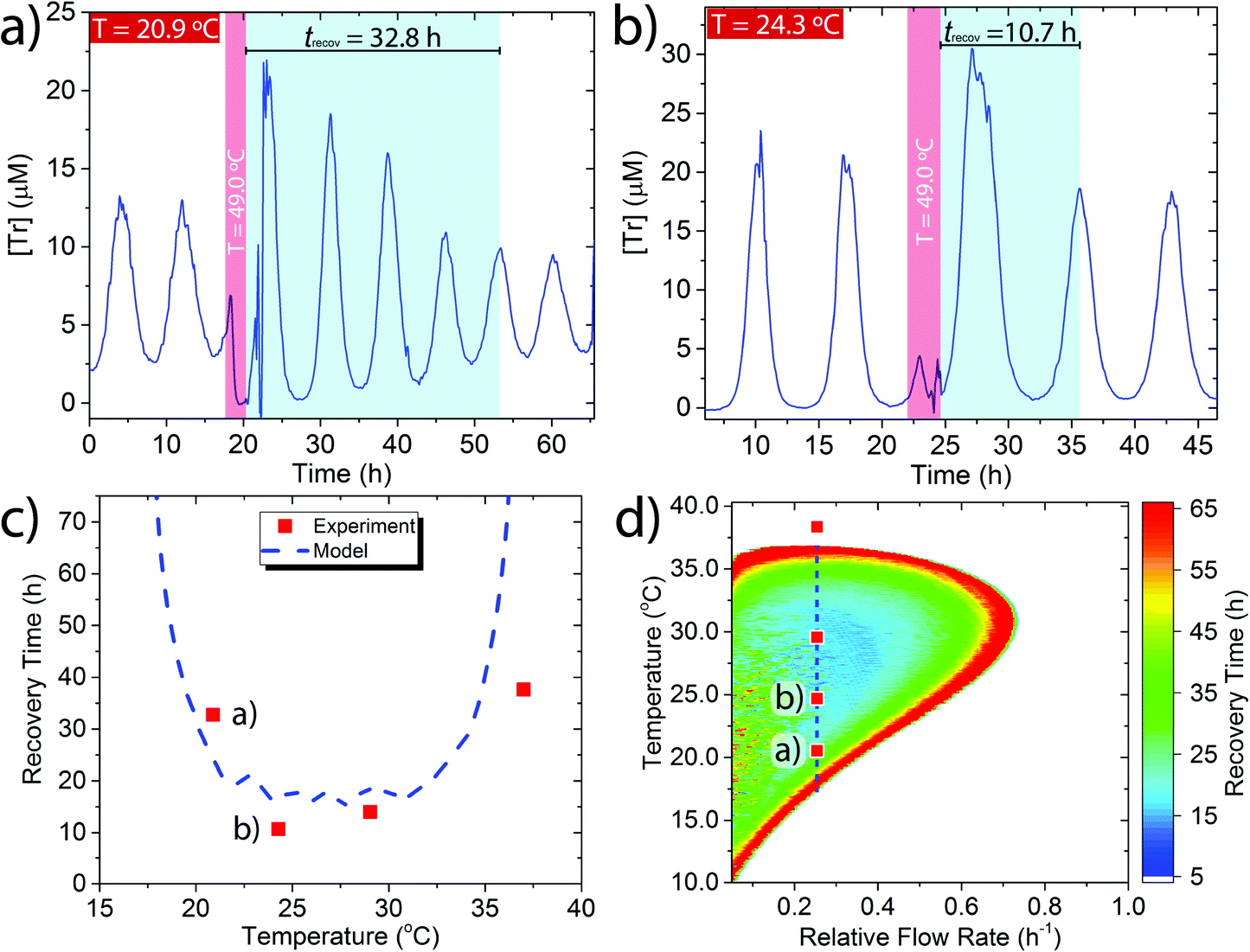Fig. 2 Perturbation-recovery experiments for temperatures T_b = (a) 20.9 °C and (b) 24.3 °C at a relative flow rate k_f = 0.25 h⁻¹. Red region shows perturbation to 49.0 °C. Turquoise region shows the recovery time required to re-enter sustained oscillations. (c) Comparison of experimental and modelled recovery times at k_f = 0.25 h⁻¹. (d) Phase plot for the modelled dependency of recovery time on temperature and relative flow rate. Experimental + modelled conditions: [Tg]₀ = 148 μM, [Tr]₀ = 0.234 μM, [Pro-I]₀ = 1.00 mM, [Ap]₀ = 0.20 U mL⁻¹.

We complemented the experimental data by modelling the effect of perturbations upon the recovery time using the previously reported temperature dependent rate equations (see ESI† Section 4 for details).²⁴ A comparison between the experimental and modelled results showed reasonable agreement (Fig. 2c). The modelling indicates that as the base temperature is moved towards the extremes of where sustained oscillations are possible then a perturbation that raises the temperature to 49 °C for 2 h can lead to a recovery time of t_recov > 70 h. Due to experimental impracticalities we did not explore the very edges of the sustained regime experimentally.

To further understand how the recovery time varied as a function of both temperature and flow rate we modelled the entire flow space over which the system produces sustained oscillations (Fig. 2d). In the coloured region of Fig. 2d the system produces sustained oscillations and the colours indicate the different length of recovery times at particular temperatures and flow rates. Outside the coloured region the system undergoes dampened oscillations into a steady state concentration. This phase plot shows that at the centre of the sustained regime, which is the furthest point from the boundary, the recovery time from a perturbation is short, t_recov = 10–15 h. Upon moving to the edges of the sustained regime, for all conditions, the recovery time increases and eventually reaches a t_recov > 70 h. A similar trend was also observed for a simulated perturbation to 5 °C for 2 h (Fig. S7, ESI†). Thus, the trypsin oscillator displays the characteristic early warning signal of critical slowing down when the oscillatory behaviour is close to collapse.^2,3 The critical slowdown occurs along the whole boundary between oscillatory and steady state behaviour and therefore under any set of conditions the network is always sensitive to its proximity to behavioural change.

The phase plot is also indicative of the differences in the sensitivity of the network to temperature perturbations under different conditions. At the centre of the sustained regime (blue region) the network is least sensitive as it recovers its original oscillations quicker than at the edge (red region), where the network is more sensitive to temperature perturbations.

In addition to the active sensing method demonstrated above we also sought a passive sensing method. Early warning signals can also arise from changes in the shape of a system's behaviour.^3,10,11 We examined the shape of the oscillation waves and how this varied in relation to the systems proximity to the boundary between sustained oscillations and steady state behaviour. We quantified changes in shape through calculating the Full Width Half Maximum (FWHM) of the oscillations shown in Fig. S5 (ESI†). We observed that the FWHM increased, i.e. the peaks broadened, as the system was moved closer to the boundary (Fig. 3a black points). We complemented our experimental results with mathematical modelling (Fig. 3a red dashed line, see ESI† Section 5). The modelled results replicate the experimental trend, however the modelled results have a smaller FWHM than that observed in experiments. The modelling clearly demonstrates that as the base temperature is shifted towards the boundary between sustained oscillations and steady state concentration behaviour that the FWHM increases as the shape of the oscillations broadens.

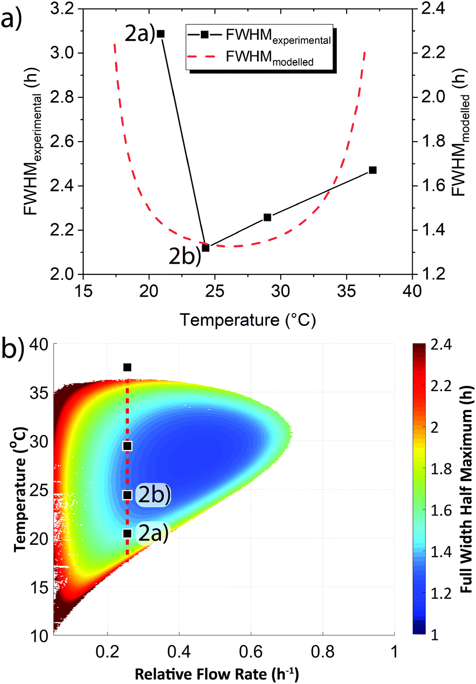Fig. 3 The change in the shape of the oscillation waves, as quantified by the Full Width Half Maximum (FWHM), brought about through changes in temperature and flow rate. (a) Comparison of experimental and modelled FWHM at k_f = 0.25 h⁻¹. Note that the modelled y-axis is off-set by 0.8 h relative to the experimental y-axis. (b) Phase plot for the modelled dependency of the FWHM on temperature and relative flow rate. Experimental and modelled conditions: [Tg]₀ = 148 μM, [Tr]₀ = 0.234 μM, [Pro-I]₀ = 1.00 mM, [Ap]₀ = 0.20 U mL⁻¹.

We modelled how the FWHM varied across the whole flow and temperature space that produced sustained oscillations (Fig. 3b). The phase plot demonstrates that as the system transitions out from the centre of the sustained oscillation region the oscillation peaks alter their shape from a narrow to a broad form. The universality of this broadening, in that it occurs irrespective of whether the temperature is raised/lowered or whether flow rates are increased/decreased, demonstrates the increase in FWHM can act as an early warning signal. In addition to the effect of temperature on the FWHM, an examination of some of our previously reported experimental results²⁴ confirmed that as the flow rate is changed and the system approaches the edge of the sustained oscillation region an increase in FWHM occurred (Fig. S6, ESI†).

The early warning signalling methods identified here provide tools by which the stability of the system may be probed without the need to comprehensively model the behaviour of the network. For example, by either comparing the recovery times after a perturbation of the network operating at two different conditions, or, by comparing the shape of the oscillations via the FWHM at two different conditions a judgement can be made about which condition is more stable and hence identify the direction in phase space where the location of highest stability is to be found.

In our study we have undertaken a joint experimental and mathematical assessment of the response of a reaction network as it is brought towards a boundary between two different behaviours. We have shown that networks reveal their proximity to a collapse transition when probed by either an active sensing method in the form of a critical slowdown in the recovery time after a perturbation and/or a passive sensing method in the form of peak broadening. Our work demonstrates that a minimal complex system based upon a single reaction network motif^25,26 produces early warnings signals. The manifestation of critical slowdown behaviour in both a simple bottom-up constructed oscillatory network built upon enzymes and small molecules (as well as in bistable systems^27–30) and in microorganisms^31,32 is encouraging as it means that reaction networks constructed out of these components with any level of complexity in-between a minimal network to a full organism will also display such early warning signals.

In the future design of complex reaction networks these early warning systems could be used to sense the stability of the system towards its environment as an input for a homeostatic feedback mechanism. The two early warnings signals demonstrated here are by no means exhaustive and many more types of EWS exist.² As chemists begin to construct more complex systems they should bear in-mind these phenomena and how they may be harnessed. The similarity in the behaviour of chemical systems and other complex systems e.g. ecosystems and financial markets, shows that the examination of other systems can be a fruitful source of inspiration for systems chemistry.

This work was supported by funding from the Simons Collaboration on the Origins of Life (SCOL [award 477123], [WTSH]) and funding from the Dutch Ministry of Education, Culture and Science (Gravity programme, 024.001.035, and a NWO Rubicon grant 019.172EN.017).

Conflicts of interest

There are no conflicts to declare.

Notes and references

1. M. Scheffer, Critical Transitions in Nature and Society, Princeton University Press, 2009.
2. M. Scheffer, et al. , Nature, 2009, 461, 53–59.
3. M. Scheffer, et al. , Science, 2012, 338, 344–348.
4. U. Feudel, A. N. Pisarchik and K. Showalter, Chaos, 2018, 28, 033501.
5. I. A. van de Leemput and M. Scheffer, et al. , Proc. Natl. Acad. Sci. U. S. A., 2014, 111, 87–92.
6. P. E. McSharry, L. A. Smith and L. Tarassenko, Nat. Med., 2003, 9, 241–242.
7. D. S. Bates, J. Finance, 1991, 46, 1009–1044.
8. S. N. Semenov, A. S. Y. Wong, R. M. van der Made, S. G. J. Postma, J. Groen, H. W. H. van Roekel, T. F. A. de Greef and W. T. S. Huck, Nat. Chem., 2015, 7, 160–165.
9. V. Dakos and M. Scheffer, et al. , PLoS One, 2012, 7, e41010.
10. C. F. Clements, J. L. Blanchard, K. L. Nash, M. A. Hindell and A. Ozgul, Nature Ecology & Evolution, 2017, 1, 0188.
11. S. Kéfi and M. Scheffer, et al. , PLoS One, 2014, 9, e92097.
12. G. Ashkenasy, T. M. Hermans, S. Otto and A. F. Taylor, Chem. Soc. Rev., 2017, 46, 2543–2554.
13. N. Srinivas, J. Parkin, G. Seelig, E. Winfree and D. Soloveichik, Science, 2017, 358, 1401.
14. S. N. Semenov, L. J. Kraft, A. Ainla, M. Zhao, M. Baghbanzadeh, V. E. Campbell, K. Kang, J. M. Fox and G. M. Whitesides, Nature, 2016, 537, 656–660.
15. R. Roszak, M. D. Bajczyk, E. P. Gajewska, R. Hołyst and B. A. Grzybowski, Angew. Chem., Int. Ed., 2019, 58, 4520–4525.
16. T. Fujii and Y. Rondelez, ACS Nano, 2013, 7, 27–34.
17. J. Leira-Iglesias, A. Tassoni, T. Adachi, M. Stich and T. M. Hermans, Nat. Nanotechnol., 2018, 13, 1021–1027.
18. A. M. Tayar, E. Karzbrun, V. Noireaux and R. H. Bar-Ziv, Proc. Natl. Acad. Sci. U. S. A., 2017, 114, 11609–11614.
19. I. Maity, N. Wagner, R. Mukherjee, D. Dev, E. Peacock-Lopez, R. Cohen-Luria and G. Ashkenasy, Nat. Commun., 2019, 10, 4636.
20. A. Padirac, T. Fujii, A. Estévez-Torres and Y. Rondelez, J. Am. Chem. Soc., 2013, 135, 14586–14592.
21. A. S. Zadorin, Y. Rondelez, G. Gines, V. Dilhas, G. Urtel, A. Zambrano, J.-C. Galas and A. Estevez-Torres, Nat. Chem., 2017, 9, 990–996.
22. S. M. Morrow, I. Colomer and S. P. Fletcher, Nat. Commun., 2019, 10, 1011.
23. B. Helwig, B. van Sluijs, A. A. Pogodaev, S. G. J. Postma and W. T. S. Huck, Angew. Chem., Int. Ed., 2018, 57, 14065–14069.
24. O. R. Maguire, A. S. Y. Wong, M. G. Baltussen, P. van Duppen, A. A. Pogodaev and W. T. S. Huck, Chem. – Eur. J., 2020, 26, 1676–1682.
25. S. S. Shen-Orr, R. Milo, S. Mangan and U. Alon, Nat. Genet., 2002, 31, 64–68.
26. U. Alon, Nat. Rev. Genet., 2007, 8, 450–461.
27. N. Ganapathisubramanian and K. Showalter, J. Phys. Chem., 1983, 87, 1098–1099.
28. N. Ganapathisubramanian and K. Showalter, J. Chem. Phys., 1986, 84, 5427–5436.
29. G. Dewel, P. Borckmans and D. Walgraef, J. Phys. Chem., 1985, 89, 4670–4672.
30. J. P. Laplante, P. Borckmans, G. Dewel, M. Gimenez and J. C. Micheau, J. Phys. Chem., 1987, 91, 3401–3405.
31. A. J. Veraart, E. J. Faassen, V. Dakos, E. H. van Nes, M. Lürling and M. Scheffer, Nature, 2012, 481, 357–359.
32. L. Dai, D. Vorselen, K. S. Korolev and J. Gore, Science, 2012, 336, 1175.

---

Footnote

† Electronic supplementary information (ESI) available. See DOI: 10.1039/d0cc01010c

---