
 Open Access Article
 This Open Access Article is licensed under a
 Creative Commons Attribution 3.0 Unported Licence
Plate-height model of ion mobility-mass spectrometry†
Márkó
Grabarics
 *ab,
Maike
Lettow
ab,
Ansgar T.
Kirk
c,
Gert
von Helden
b,
Tim J.
Causon
d and
Kevin
Pagel
*ab
*ab,
Maike
Lettow
ab,
Ansgar T.
Kirk
c,
Gert
von Helden
b,
Tim J.
Causon
d and
Kevin
Pagel
*ab
aDepartment of Biology, Chemistry and Pharmacy, Institute of Chemistry and Biochemistry, Freie Universität Berlin, Takustrasse 3, 14195 Berlin, Germany. E-mail: grabarics@fhi-berlin.mpg.de; kevin.pagel@fu-berlin.de
bFritz Haber Institute of the Max Planck Society, Department of Molecular Physics, Faradayweg 4-6, 14195 Berlin, Germany
cInstitute of Electrical Engineering and Measurement Technology, Department of Sensors and Measurement Technology, Leibniz Universität Hannover, Appelstrasse 9A, 30167 Hannover, Germany
dDepartment of Chemistry, Institute of Analytical Chemistry, University of Natural Resources and Life Sciences, Vienna, Muthgasse 18, 1190 Vienna, Austria
First published on 8th July 2020
Abstract
In the past decade, ion mobility spectrometry (IMS) in combination with mass spectrometry (IM-MS) became a widely employed technique for the separation and structural characterization of ionic species in the gas phase. Similarly to chromatography, where studies on the mechanism of band broadening and adequate plate-height equations have been aiding method development and promoting advancements in column technology, a suitable resolving power theory of drift tube ion mobility-mass spectrometry (DTIM-MS) is essential to stimulate further progress in this emerging field of separation science. In the present study, therefore, we explore dispersion processes in detail and present a plate-height model of ion mobility-mass spectrometry. We quantify the effects of five major dispersion processes that contribute to zone broadening and determine the resolving power in DTIM-MS: diffusion, Coulomb repulsion, electric field inhomogeneities, the finite initial spread of the ion cloud and dispersion outside the mobility cell. A solution is provided to account for the nonuniform separation field in IM-MS in the presence of multiple compartments. The equations – derived from first principles – serve as the basis for formulating an expression that is similar in nature to van Deemter's plate-height equation for chromatography. A comprehensive set of experiments was performed on a custom-built DTIM-MS instrument to evaluate the accuracy of the plate-height model, resulting in satisfactory agreement between experiment and theory. Building on these findings, the plate-height equation was employed to explore the influence of drift gas pressure, injection pulse-width and the mobility of ions on resolving power from a theoretical point of view. Our findings may aid instrument design and development in the future, as well as the optimization of measurement conditions to improve ion mobility separations. By employing the plate-height concept and the general formalism of differential migration processes to describe zone spreading in IM-MS, we aim to find a common ground between this emerging method and such well-established techniques as HPLC or CZE. We also hope that the work presented here will facilitate a broader acceptance of IMS as a separation method of great potential by the communities of chromatography and electrophoresis, as well as that of mass spectrometry.
1. Introduction
With the advent of commercially available instruments of various designs, ion mobility-mass spectrometry (IM-MS) has emerged from being a method used by a handful of academic research groups – mainly in the fields of chemical physics and gas-phase ion chemistry – to become a widely employed technique in analytical laboratories. Therefore, evaluating the performance of IM-MS as an analytical method capable of separating ionic species based on their mass, charge, size and shape is of high interest. The purpose of the present study is to assess the efficiency of IMS/IM-MS as a separation method that is based on the differential migration of ions through a mobility cell. A plate-height model of drift tube IM-MS, built on a macroscopic view of ion mobility separations, is presented. The frame of the plate-height model helps us underline differences and similarities between this emerging technique and such well-established differential migration methods as capillary zone electrophoresis (CZE) or high-performance liquid chromatography (HPLC).In analogy to the description of distillation and extraction in fractionating columns,1 Martin and Synge developed the plate theory of chromatography2–4 to describe the elution process and the evolution of chromatographic bands. Although more advanced macroscopic and microscopic theories have been developed since, such as the differential mass balance equations5 (forming the basis of the Van Deemter equation6) or the stochastic theory of chromatography,7–13 the concept of plate numbers and plate heights remained central in the field. This well-established concept provides a set of highly useful definitions, such as those of peak-to-peak resolution and peak capacity, making the evaluation of the efficiency of separations convenient and consistent. By defining the plate number and the plate height in a more general and abstract manner that is not linked directly to distillation, extraction or partition processes (i.e. to real or virtual equilibration stages in the column), Giddings made this thoroughly developed concept accessible for other differential migration methods of separation.14,15 Therefore, although linear IMS and column chromatography have fundamental differences (the first one being an electrophoretic, the second a partition/adsorption process), zone broadening in the two techniques can be described employing the same formalism. When nonlinear effects are absent, chromatographic peaks converge toward a Gaussian profile, and the total variance of this distribution is the sum of the variances corresponding to the individual dispersion processes. These conditions form the basis for the application of plate-height models. As the aforementioned criteria are satisfied in drift tube ion mobility spectrometry (DTIMS) and drift tube ion mobility-mass spectrometry (DTIM-MS) as well, the plate-height concept can be utilized to address peak broadening. The dispersion processes that determine broadening in chromatography and IM-MS, of course, are fundamentally different, but the framework is the same and the fruitful analogy between the two aforementioned techniques can be harnessed as long as the linearity of the system is maintained.
In the first part of the study, a macroscopic model is presented that describes the spatial spread of ion clouds during ion mobility separations (section 3). The model addresses the most important processes that contribute to zone spreading in DTIM-MS: diffusion, Coulomb repulsion, electric field inhomogeneities, the finite initial spread of the ion cloud and broadening after the mobility cell. Equations derived from first principles to quantify the effects of these intrinsic and extrinsic processes that contribute to dispersion are presented and interpreted in detail. Following the description of the model, the findings are synthesized employing the plate-height concept to yield a formula that is analogous to van Deemter's equation for chromatography6 (section 4.1). We employ the aforementioned equation to calculate the resolving power of a custom-built drift tube ion mobility-mass spectrometer under a variety of defined operating conditions, and the results are compared to those obtained experimentally in a series of systematic measurements (section 4.2). The plate-height model is found to reproduce experimental results with satisfying accuracy, validating the theory and the suitability of the approach. Finally, employing the plate-height equation, calculations are performed to explore the role of the drift gas pressure, the injection pulse-width and the mobility of the ions in determining the resolving power of IM-MS (section 4.3). For this purpose, a representative set of hypothetical analytes – spanning over a wide range of sizes and charge-states – were chosen to emphasize the generality of the theory.
1.1. Figures of merit in the plate-height model
To quantify the effects of different contributors to peak broadening in IM-MS and to compare this method to other separation techniques, one requires a suitable framework and indices that are accurate measures of the performance of separation methods. For this purpose, a linear static model of theoretical plates and plate height (inherited from chromatography) was chosen. The most important figures of merit that are used throughout this article – namely variance, number of theoretical plates, resolving power, and the height equivalent to a theoretical plate – are defined and described in detail below.(I) Let us first address the shape, width and statistical variance associated with distributions and peaks. Since drift tubes and TWIMS cells serve as Gaussian operators (similarly to columns in chromatography), peaks in IMS approach a Gaussian lineshape. It should be noted that even though peaks in chromatography and IMS are never truly Gaussian, they converge toward this distribution. Therefore, it is a convenient and widely-accepted approximation to describe them using the normal distribution, although in the case of chromatography the exponentially modified Gaussian (EMG) is a more accurate model. The width of a Gaussian in separation methods can be expressed using the distribution's standard deviation (σ), and is generally defined either in time (2σt, termed temporal width) or in space (2σL, spatial width). The widths defined this way equal the distance between the two inflection points of the Gaussians, measured either in the temporal- or in the spatial domain, respectively. The relation between σt and σL is given by the velocity of the ion packets.
The quantities σt2 and σL2 are generally employed to express dispersion in plate-height models and we refer to them as the temporal- and spatial variance, respectively. In case individual dispersion processes are considered to act independently, such as in DTIM-MS, the variances corresponding to them are additive. The resulting overall temporal variance of a given arrival time distribution (ATD), or the spatial variance of the corresponding zone arises as the sum of the appropriate variances associated with the individual dispersion processes.
(II) The number of theoretical plates (N) is a universally accepted dimensionless quantity to describe peak broadening, given by definition as:
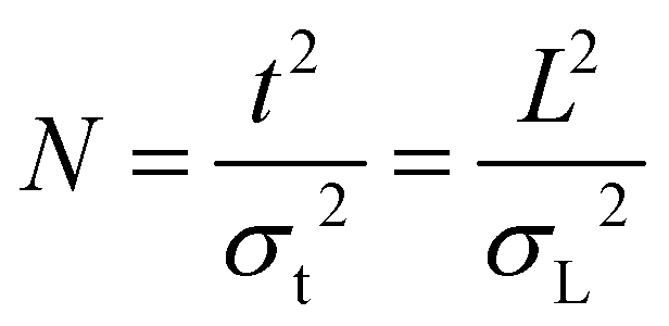 | (1) |
Here, t is the time a given ion cloud or band spends in the separation field (time of separation; for example, drift time, arrival time or retention time), while L is its equivalent in space (length of the separation field, i.e. the distance covered during the migration process). Time and length domains are not to be confused and one needs to be consistent when using them in order to end up with a dimensionless quantity. Eqn (1) also gives the relation between σt2 and σL2. If a distribution or peak is not sufficiently close to a Gaussian, it is more accurate to employ statistical moment analysis (analysis of the shape of the distribution) and obtain the variance by calculating the second central moment of the distribution rather than deriving it from the distance between the inflection points.16–18 The theoretical plate was originally introduced to describe distillation processes and it does not have a real physical meaning in the case of differential migration techniques (chromatography, electrophoresis, capillary electrochromatography, field-flow fractionation, time-of-flight and distance-of-flight mass spectrometry, ion mobility spectrometry, etc.). However, it is a very useful index that provides a frame for comparing the performance of different methods. In the case of IMS and IM-MS, N can be interpreted as the square of the displacement of the ion cloud corresponding to a peak in relation to the variance that is generated during the displacement. In other words, it is a measure of “resistance toward broadening”, as N expresses the ratio of two antagonistic processes: migration (directional and beneficial) and dispersion (random and detrimental). The aforementioned resistance, however, is not an intrinsic property of a given compound, but characteristic to the separation and to the behavior of the analyte during this process. Although N is generally used to evaluate and compare the performance of techniques, it is always calculated for a given analyte and can be different for different species undergoing the same separation process.3 In other words, it depends on both the measurement conditions and on the nature of the analyte. As N is inversely proportional to variance, reciprocal plate numbers are additive, provided L and t are the same for all dispersion processes considered. Satisfying this criterion is not trivial when post-cell processes lead to a nonuniform separation field. An appropriate solution for such situations is given in section 3.5.
(III) The height equivalent to a theoretical plate (HETP) – also termed simply plate height (H) – is the ratio of the length of the separation field and the number of theoretical plates.1 To give a more general, abstract definition proposed by Giddings, HETP can be interpreted as the rate of generating variance or, in other words, zone spreading per unit length:14,15
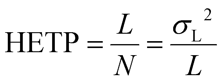 | (2) |
HETP is directly proportional to spatial variance and has a dimension of length. Since HETP is generally used in column chromatography, most prominently in the well-known plate-height equations of van Deemter6 and Giddings19 that show the contribution of the individual dispersion processes in an elegant way, we also employ it to formulate the analogous expressions.
(IV) Another dimensionless figure of merit to evaluate the performance of separations is resolving power (Rp):
 | (3) |
Here, wh is the full-width-at-half-maximum (FWHM) of a distribution, expressed as either a temporal or a spatial quantity. Rp is analogous to N, and in case of a Gaussian distribution the relation between the two figures of merit is the following:
 | (4) |
The number in the denominator stems from the relation between σ and wh for normal (Gaussian) distributions  . Although the relation between Rp and N might imply that Rp−2 is also an additive quantity, one must be careful. As Rp is defined based on the FWHM of distributions, not on variances, the addition of Rp−2 involves the addition of FWHM squared values (wh2). This quantity, however, is not necessarily an additive one: wh2 values add linearly only in the specific case when all of the distributions are Gaussians (and the underlying processes act independently). Summation of the square of FWHM values when at least one of them corresponds to a different type of distribution (rectangular, quadratic, etc.) contradicts the central limit theorem of statistics20 and leads to incorrect results. Since some of the dispersion processes in IM-MS are characterized by non-Gaussian distributions (most importantly the injection pulse that is generally described as a rectangular function), care must be taken. In other words, the total width of the peaks and the corresponding overall resolving power cannot be calculated by adding the wh2 values of the individual dispersion processes together when not all of them are characterized by a normal distribution. This important issue has been often overseen when employing the conditional resolving power theory of IMS (and, consequently, also in the semi-empirical resolving power model, as it is based on the former one). Shortcomings of the aforementioned theories that stem from this oversight are addressed in more detail in the ESI, section S1.†
A possibility to overcome the above-described problem and render resolving power limit to a dispersion process with non-Gaussian distribution (such as the injection pulse-width) is to calculate the FWHM of a normal distribution that has the very same variance as the non-Gaussian distribution in question, and use the FWHM value of this virtual Gaussian to obtain the correct Rp limit. In other words, the variances of non-Gaussian distributions are obtained using statistical moment analysis, the plate number limits of these dispersion processes are calculated using the definition of N, and the corresponding limits of Rp are obtained employing eqn (4). This solution is mathematically equivalent to the addition of variances, and completely justified as long as the observed ATD is sufficiently close to a Gaussian profile. In the present study, the described solution is employed to incorporate resolving power into the plate-height model and to formulate the appropriate equations.
Because plate heights and theoretical plates are directly related to variance, it is more convenient and fortunate to employ them when evaluating the efficiency of separations. Although resolving power is not traditionally employed as a figure of merit within plate-height models in chromatography, electrophoresis, etc., we included it into the plate-height model of IM-MS due to its widespread application in the IMS community. Thus, to conform to the conventions of both fields, in the present study HETP, N and Rp will be used in parallel.
2. Experimental section
2.1. Materials and methods
Dextran from Leuconostoc mesenteroides (analytical standard, for GPC, average Mw 1000) was purchased from Fluka; tetrabutylammonium iodide (≥99.0%) and 12-crown-4 (98%) were purchased from Sigma-Aldrich. The compounds were dissolved in water/methanol 50/50 (v/v) solution containing 0.1% formic acid in the following concentrations: dextran 1 mg mL−1; tetrabutylammonium iodide (TBAI) 200 μM; 12-crown-4 500 μM. The following three singly-charged cations were chosen for the experiments: protonated 12-crown-4 (nominal m/z = 177, DTΩHe = 74 Å2), sodium adduct of dextran-derived trisaccharide (nominal m/z = 527, DTΩHe = 139 Å2) and TBAI trimer cation [(TBA)3I2]+ (nominal m/z = 981, DTΩHe = 270 Å2). The analytes are commercially available standards, yield symmetric ATDs and the ratio of the ions’ mobilities is approximately 1![[thin space (1/6-em)]](https://www.rsc.org/images/entities/char_2009.gif) :2:4 (equirational progression).
:2:4 (equirational progression).
Data processing was carried out using an in-house developed LabView software, while data analysis and calculations were performed using Origin 2017 software package (OriginLab Co.). ATDs were fitted with Gaussian function (employing Levenberg–Marquardt least-squares minimization algorithm) to allow for the determination of arrival times (corresponding to the peak centroid), full-width-at-half-maxima (wh) and standard deviations (σ). Rotationally-averaged collision cross sections were determined using the stepped-field method and the Mason–Schamp equation.
2.2. Ion mobility-mass spectrometry measurements
A schematic representation of the custom-built DTIM-MS instrument employed to obtain the experimental data in the present study is shown in Fig. 1.21 A device of very similar design has also been described in detail by the Bowers group.22 The ions – generated using a nanoelectrospray ion source (nESI) and Pt/Pd-coated borosilicate capillaries prepared in-house – are collected, radially focused and trapped by a ring-electrode radiofrequency ion funnel. This four-stage entrance funnel also served to inject discrete ion clouds with defined pulse-width and injection voltage (30 V) at a rate of 10–20 Hz into the 805.5 mm-long drift region. The latter consists of similar segments of conductive glass tubes (Photonis, USA) and was operated at ambient temperature (295.0 ± 0.2 K, monitored with a PT100 temperature sensor attached to the drift cell) in the pressure range from 3 to 5 mbar during the experiments, using helium as buffer gas (99.999% purity). Being critical in IMS experiments, the buffer gas pressure was monitored with a high-precision MKS Baratron absolute pressure gauge (type 627). To avoid the contamination of the high-purity buffer gas inside the drift tube, a constant pressure difference of 0.60 mbar was maintained between the drift region and the entrance funnel. The drift field was varied between 2.0 V cm−1 and 14.4 V cm−1 in the measurements, corresponding to reduced electric fields between 1.6 and 19.3 Td. A second electrodynamic ion funnel (exit funnel, 144 mm in length) enables the radial confinement of ion clouds after the drift cell and facilitates the transport of ions through the conductance limit (the pressure and temperature in the exit funnel is identical to that inside the drift region). Ions are then transmitted through two differentially pumped stages by ring-electrode guides before reaching the high vacuum region of the instrument. Here a quadrupole mass filter and another quadrupole ion guide of identical dimensions enables m/z-selection and the efficient transport of ions. The ions then pass an einzel lens stack and a set of steering lenses before finally being detected using an off-axis electron multiplier. Another possibility offered by the setup is to pulse the ions into an orthogonal Wiley–McLaren time-of-flight mass analyzer before subsequent detection. This latter operation mode, however, was not utilized in the present study, as it only allows for the sampling of the ATDs at a much lower rate due to the time-of-flight analysis. In spite of the unique design, the instrument is similar and comparable to commercially available DTIM-MS devices. Together with the fact that the presented theoretical model is highly general and not based on specific considerations regarding instrument design, the findings bear relevance to any other DTIMS and DTIM-MS setup. | ||
| Fig. 1 Schematic drawing of the custom-built DTIM-MS instrument used in the experiments. | ||
3. Theoretical model
In the following section each dispersion process that contributes to zone spreading in DTIM-MS is addressed individually. Equations that quantify the effects of the most important intrinsic and extrinsic contributors are derived and interpreted in detail. Only the most important equations are presented here, while detailed derivations can be found in the appropriate parts of the ESI,† as indicated. At the end of the section we also provide a brief comparison between the plate-height model developed herein and its counterparts for chromatography and electrophoresis. The findings described here will enable the formulation of an expression that is similar in nature to van Deemter's equation for chromatography, presented in the Results and discussion section. Therefore, if the detailed description of the model is not of the reader's main interest, they can directly continue with section 4.In relation to peak broadening, it is important to mention that peaks are not present in the mobility cell and are abstract by their nature. Peaks or ATDs only arise when the analytes reach the detector and generate a response signal as a function of time. On the other hand, zones – formed by the ion clouds or ion packets – consist of the actual analytes and traverse the separation field. In the present study, the expressions peak broadening and zone broadening or zone spreading are used in accordance with the nomenclature of chromatography and electrophoresis.15 A suitable alternative might be ion cloud broadening, but it is not our aim to establish such novel terms for IMS. Finally, it should be emphasized that the following equations are only valid in the low-field regime, whereby the ions are assumed to be in thermal equilibrium with the buffer gas and, consequently, the ion mobility (K) is not a function of the electric field strength.23
3.1. Intrinsic contributors I. Diffusion
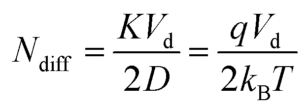
Longitudinal diffusion has been identified in IMS and IM-MS as the most important and dominant among the intrinsic contributors – processes that cause dispersion inside the mobility cell.23–25 Considering only a few fundamental equations of Einstein and Townsend, calculating diffusional broadening is straightforward (ESI, section S2†).The spatial and temporal variance generated due to diffusional broadening is given as:
 | (5a) |
 | (5b) |
In the above expressions Ld is the length of the drift cell, td is the drift time, Vd is the drift voltage, T is the absolute temperature, D is the diffusion coefficient of the ion while K is its mobility, kB is the Boltzmann constant and q is the charge of the ion (q = ze, where z is the charge-state and e is the elementary charge). The two variances are not equal, neither regarding their numerical values, nor their units. Eqn (5a) refers to a spatial quantity, while eqn (5b) expresses variance in the time domain. According to their definition, the diffusion limit of plate number and resolving power can be readily calculated from eqn (5a) or (5b):
 | (6) |
 | (7) |
The above results are analogous to those of zone electrophoresis, for which the corresponding equations were first derived in 1969.14 Since diffusional broadening leads to Gaussian distributions, employing the relation given in eqn (4) to derive resolving power from the number of theoretical plates in fully justified. Eqn (6) and (7) express precisely what Giddings described so eloquently in his magnum opus: “Separation is the art and science of maximizing separative transport relative to dispersive transport”.15 In this case, the directional motion of ions due to an electric field is responsible for separative (also termed differential) transport, and is proportional to K. On the other hand, random thermal motion causing diffusion (the corresponding transport property being D) is responsible for dispersive (entropic) mass transport.26 One can also interpret eqn (6) as the ratio of an electrical energy – the electrical potential energy drop experienced by the ions (qVd) – and the thermal energy (kBT).14,27
Eqn (6) makes it apparent that the diffusion limit of theoretical plates is directly proportional to the applied drift voltage (within the low-field limit), a measurement parameter the analyst has under complete control. Second, it also depends on the ratio of two transport properties, the mobility and the diffusion coefficient of the ion, not on their absolute values. This ratio is entirely independent of the collision cross section and depends only on the temperature and the charge of the species. Thus, decreasing the temperature in the mobility cell leads to increased resolving power.28–30 It is interesting to recognize that the diffusion limit of the plate number/resolving power is entirely independent of analysis time and the pressure inside the mobility cell. These variables are not involved in eqn (6) and (7), neither explicitly, nor implicitly. Although both K and D depend on p, they depend on it in the same way, meaning that the effect of pressure cancels out.
It is also evident that Ndiff and Rp;diff do not depend explicitly on the length of the mobility cell. Since the exponents of Ld and Ed (the drift field, i.e. the strength of the electric field inside the drift cell) are equal in eqn (6) and (7), and they are inversely proportional (yielding EdLd = Vd), applying the same drift voltage on a longer drift tube will not increase the diffusion limit of resolving power. However, since the upper limit of the low-field regime is determined by the  ratio, with n being the drift gas number density, longer drift tubes and higher pressures in the mobility cell allow for the application of higher drift voltages, while maintaining operation under low-field conditions to avoid entering the realm of nonlinear IMS. Furthermore, as we shall see later when addressing other dispersion processes, employing longer drift cells and higher pressures are beneficial and have a significant, positive influence on the apparent resolving power (at the cost of reduced transmission and duty cycle). Although diffusion appears as the most important among the intrinsic dispersion processes, it is not the only factor that contributes to zone spreading in IMS.24,31–41 Consequently, the diffusion limit of resolving power is essentially never reached in practice, and eqn (5)–(7) only express the contribution of this process to total zone spreading.
3.2. Intrinsic contributors II. Coulomb repulsion
Coulombic interaction between ions and the perturbation of the electric field inside the separation region (e.g. the capillary or the drift tube) by the presence of charged species can lead to interesting phenomena in electrophoretic systems. Nonlinear effects and boundary anomalies have been extensively studied in condensed-phase electrophoresis, often in relation with conservation functions,42 the most prominent being the Kohlrausch regulating function (KRF).43 In CZE, for example, electromigration dispersion (EMD) significantly influences the shape and width of zones under normal operating conditions.44–47 EMD stems from the deviation of the field strength within the analyte zone compared to that in the background electrolyte. Local migration rates become a function of the local concentration of constituents, resulting in additional broadening and the distortion of peaks.48,49 Due to this triangulation, peaks in CZE do not converge toward a Gaussian profile and their shapes instead are described by the Haarhoff–Van der Linde (HVL) function.50–52 Moreover, as EMD and diffusional broadening do not act independently, the total variance is not the simple sum of the individual contributors, meaning that the calculation of the overall zone spreading is nontrivial and the basis for applying the plate-height model (the simple addition of variances) in CZE is often feeble and questionable.49,51Nonlinear effects in IMS are, fortunately, relatively weak in comparison to CZE, and the simplicity of plate-height models can be exploited while preserving accuracy to a satisfying level. In IMS, where electroneutrality does not hold, coulombic interactions lead to the space charge-driven expansion of ion clouds. Ionic species interact not only with the drift field (Ed), but also with each other's electric field. There are many excellent studies dealing with space charge effects in IMS,53–57 including a recent paper by Eiceman and co-workers,58 who developed and solved numerically a nonlinear integro-differential equation to account for the simultaneous dispersive effect of diffusion and Coulomb repulsion. They found that space charge effects become important when ion densities exceed 106 cm−3, in accordance with previous findings.53 At large ion densities, the simulated peaks ceased to be Gaussian and could be approximated with the Kohlrausch–Williams–Watts (KWW) function with the stretching exponent γ exceeding 2 (γ = 2 yields a Gaussian distribution). The approach is similar to fitting peaks in CZE using the HVL function, as mentioned above.
The disadvantage of such nonlinear theories is the loss of simplicity and the lack of compatibility with plate-height models, as the total variance does not appear as the sum of the variances of individual contributors. From the realization that – under conditions most IM-MS instruments operate – Coulomb-driven dispersion is significantly smaller than diffusional broadening (or electromigration dispersion in CZE), and that the total number of ions in the drift cell can often only be estimated, a profitable compromise arises. Thus, to preserve the simplicity of a linear separation system and the lucrative framework provided by the plate-height model, we employ here a simpler – albeit less accurate – solution to account for the expansion of ion clouds due to coulombic forces, following the approach of Tolmachev et al.56 In case of interest, the reader is referred to the ESI, section S3† for the detailed derivations, as only the most important expressions are presented below.
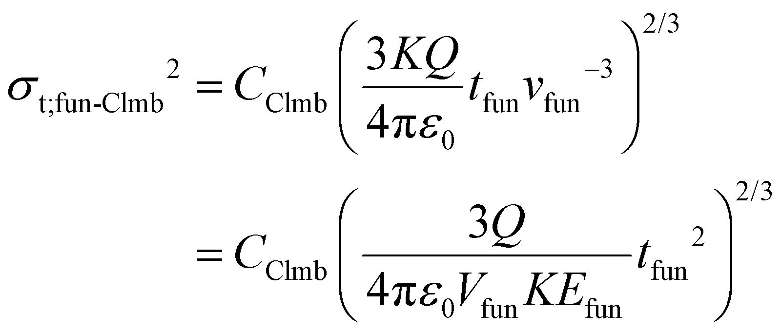
The variances associated with Coulomb-driven dispersion – considering spherical ion clouds – can be expressed as:
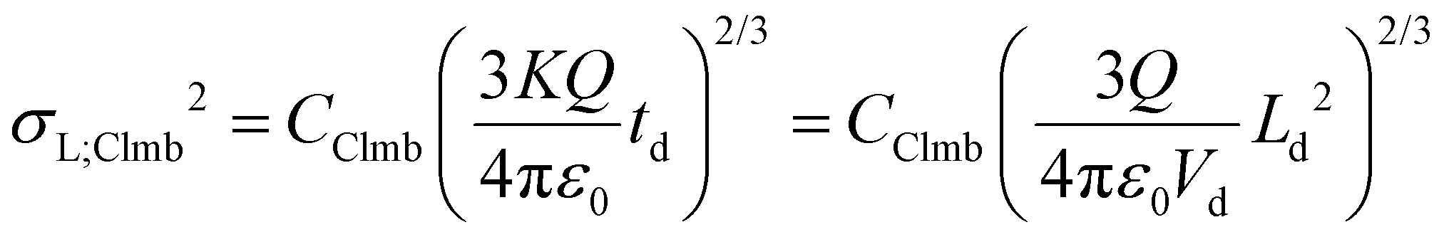 | (8a) |
 | (8b) |
In the two above equations, Q is the total charge of the ion cloud, ε0 is the vacuum permittivity (approximating the permittivity of the buffer gas in the mobility cell), while CClmb is a dimensionless constant that relates the square of the radius of the ion cloud to the spatial variance in the plate-height model. CClmb is not an experimentally determined parameter or a correction factor with an arbitrary value – it can be obtained by statistical moment analysis and reflects the distribution of ions within the cloud (for more details, see ESI, sections S3.2 and S3.3†).
Based on the above expressions of variances, the Coulomb limit of theoretical plates and resolving power can be formulated, analogously to eqn (6) and (7) for diffusion:
 | (9) |
 | (10) |
The higher the total charge confined behind the surface of the ion clouds, the lower NClmb and Rp;Clmb will be. It is interesting to compare the two above expressions with their counterparts for diffusion. Opposed to their diffusion limited equivalents, the above equations depend explicitly on the length of the drift cell. Employing higher drift voltages, on the other hand, increases both the diffusion- and the Coulomb limit of theoretical plates and resolving power. Eqn (9) and (10) also depend on the ratio of transport properties, albeit in a rather invisible way, as in this case the two transport properties in the numerator and the denominator are one and the same: the ion mobility. Because the transverse velocity of the ion clouds along the mobility cell (vd) and the rate of their free expansion (vClmb, see ESI eqn (S10)†) depend on K in the same way, the effect of ion mobility cancels out. This finding will prove to be relevant when the effects of electric field inhomogeneities are discussed.
3.3. Intrinsic contributors III. Electric field inhomogeneities
Any deviation from an ideal, homogenous electric field inside a drift tube results in increased drift times in IMS, meaning that more time is available for the ions to spread due to diffusion and space charge effects. Ions behave as if their mobility (the transport property associated with migration) is decreased, while the transport properties associated with dispersion, such as the diffusion coefficient, remain constant. Consequently, electric field inhomogeneities lead to decreased performance and resolving power in DTIMS. Moreover, such imperfections also cause a systematic error in the determination of ion mobilities and collision cross sections (Ω).21,35,59One can introduce the virtual mobility (![[K with combining low line]](https://www.rsc.org/images/entities/i_char_004b_0332.gif) ) to account for the deteriorating effect of electric field inhomogeneities inside the drift cell:
) to account for the deteriorating effect of electric field inhomogeneities inside the drift cell:
 | (11) |
Here, θ is a dimensionless factor, quantifying the degree of inhomogeneity. The more homogeneous the electric field is, the closer θ gets to 1, and the less the virtual mobility deviates from K. It is always the virtual mobility that can be directly determined using DTIMS. When deriving the diffusion coefficient from the virtual mobility using the Nernst–Townsend relation, it is not possible to obtain the actual value of D. The result will be the virtual diffusion coefficient (![[D with combining low line]](https://www.rsc.org/images/entities/i_char_0044_0332.gif) ), which is systematically and erroneously lower than the actual value of D with the factor θ:
), which is systematically and erroneously lower than the actual value of D with the factor θ:
 | (12) |
It is of course D and not that determines the rate of diffusion in the drift cell. Therefore, a correction of the Nernst–Townsend relation – the fundamental relation between ion mobility and the diffusion coefficient – is needed in the presence of electric field imperfections, the correction factor being θ. This correction expresses a decrease in the  ratio by the factor θ, lowering the diffusion limit of plate numbers and resolving power by θ and
  , respectively. Eqn (5)–(7) can be extended by θ (by substituting for K and keeping D) to account for imperfections of the electric field, analogously to the example below:
 | (13) |
Correction of transport coefficients is not unheard-of in IMS. The Townsend factor (η) is generally used to account for increased diffusional contribution caused by elevated effective ion temperatures (when ions are not in thermal equilibrium with the drift gas due to the excess energy they gain from the drift field).35,60 In this case the diffusion coefficient is increased by the Townsend factor, which leads to a decrease in the  ratio by η.
The additional time the ion clouds spend in the mobility cell due to imperfections in the electric field does not only increase their diffusional broadening, but also contributes to their coulombic force-driven expansion (see eqn (8) and eqn (S14)†). Thus, correction of eqn (8)–(10) with the factor θ can also be implemented for Coulomb repulsion. Due to a nonideal electric field in the drift cell, td will be determined by the virtual ion mobility () and not by K:
 | (14) |
Substituting eqn (14) into eqn (8a) to eliminate td from it yields:
 | (15) |
Note that the other mobility term already present in the equation remains unaffected and does not decrease to become . It reflects the rate of the Coulomb-driven expansion (proportional to EClmb, see ESI, section S3.1†) and not the transverse motion of the ion clouds along the drift cell. Out of these two velocities, only the latter one is affected by electric field inhomogeneities. As a result, the spatial variance corresponding to Coulomb repulsion is increased by a factor of θ2/3, while the corresponding Coulomb limit of theoretical plates and resolving power should be divided by θ2/3 and θ1/3, respectively. In both eqn (13) and (15) the reciprocal of θ necessarily has the same exponent as Ed (or Vd).
The equations above are based on the assumption that all ions experience the same inhomogeneous electric field. The situation, however, is more complicated if the homogeneity of the drift field varies radially: ions with different trajectories will experience a different degree of inhomogeneity.35 In other words, the virtual mobility of the ions will not be a well-defined value. Instead, it will become a distribution according to the trajectories of the ions and the variation of the field inhomogeneity in the radial coordinates. As drift velocities and drift times depend on , ATDs will need to be convoluted with the distribution of the ions’ virtual mobilities, leading to additional broadening. To quantify this effect, an accurate knowledge of the spatial map of the electric field would be required (followed by ion trajectory simulations), making it impossible to give a general solution. Moreover, the aforementioned information is usually not available, hindering even the formulation of a suitable prediction or approximation.
Theory offers a possibility to determine the degree of axial inhomogeneity if accurate reference mobility and collision cross section values were available. However, it is very difficult in practice to separate the effect of electric field inhomogeneities from other sources of systematic error. The Mason–Schamp equation – the fundamental low-field ion mobility equation – relates ion mobility to the collision cross section of an ion:23,61–63
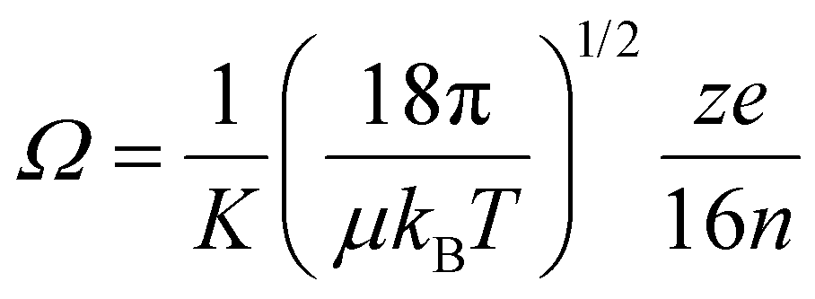 | (16) |
Here, Ω is the rotationally-averaged collision integral, also termed collision cross section, μ is the reduced mass of the ion-neutral collision complex and n is the number density of the buffer gas. A systematic, positive deviation of experimentally determined collision cross sections from reference Ω values may be indicative of the lack of an ideal, perfectly homogeneous electric field inside the mobility cell:
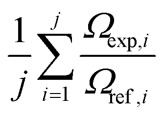 | (17) |
However, it requires the complete absence of other systematic errors, which might not be realistically achievable in practice. Moreover, as there are no collision cross section reference values available that represent such high precision and trueness as, e.g. their counterparts for mass, field inhomogeneity effects remain elusive in IMS and IM-MS.
3.4. Extrinsic contributors I. Initial spread of the ion cloud, the injection pulse-width
So far, we have explored the influence of intrinsic contributors that lead to dispersion inside the mobility cell. However, the ion clouds are not infinitesimally narrow at the moment they enter the drift tube. Similarly to the injected sample plugs in CZE, they have a finite volume and width that contributes significantly to the total variance, and as such, must be taken into account.64 In column chromatography, band broadening due to finite injection length can be reduced by focusing the analytes on the top of the column, employing, for example, performance optimizing injection sequence (POISe).65 However, as no equivalent of such a method is available for IMS, the effect of this extrinsic contributor is more pronounced.In a simple and generally accepted assumption, the initial distribution of ions follows the shape and width of the injection voltage pulse, which is usually applied as a step function (rectangular, also called uniform distribution). Although not always entirely valid, this assumption has been considered in most studies dealing with the role of the injection pulse-width and will also be employed herein, keeping in mind its limitations. Table 1 summarizes the variances of different initial distributions. The closer these distributions are to a Dirac delta-function (representing an infinitesimally narrow distribution where tinj and the corresponding variances are zero), the closer the overall resolving power approaches the limit determined by the unavoidable dispersion processes of diffusion and Coulomb repulsion.
| Distribution | Temporal variancea | Spatial varianceb |
|---|---|---|
| a t inj corresponds to the full temporal width of the injection, i.e. to the time duration of the gating voltage pulse. b Due to the following relations: σL/L = σt/t and σL = σtv. Here E represents the effective electric field strength accelerating the ions upon injection into the separation region. E is essentially equal to the drift field and can be calculated as the ratio of the drift voltage and the length of the mobility cell, because the voltage drop along the drift tube is linear. Moreover, the ions are immediately thermalized and lose their initial velocity they gained from the injection voltage due to the large number of collisions they experience with the buffer gas in the mobility cell. c Based on the convention that for a Gaussian the width at the baseline equals 4σ. | ||
| Rectangular |
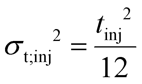
|

|
| Gaussianc |

|
|
| Quadratic |

|

|
| Triangular (isosceles) |

|

|
In relation to the injection pulse-width, it is important to comment on the semi-empirical resolving power theory.35 In the aforementioned model a dimensionless factor (β) is obtained by a fitting procedure to correct for the difference between the theoretical (optimal) width and the actual width of the injected ion packet. Herein, we present the correct values of the β coefficient in the ideal cases (i.e. when the theoretical and actual spread of the initial distribution is the same), as there has been some confusion regarding this issue in the IMS and IM-MS communities. Generally, two variants of the semi-empirical resolving power theory are being used in the literature. In the first case, β is defined as the proportionality factor between two temporal wh;t2 values. One corresponds to the theoretical wh;t2 of the initial distribution, the other to the actual, experimentally determined wh;t2. If the initial distribution is assumed to be Gaussian, the ideal value of β appears to be 1, representing the case when the actual width equals the theoretical one.
In the other, more widespread variant of the semi-empirical model, the theoretical width of the initial distribution is not given as its FWHM. Instead, it is measured at the baseline, i.e. it corresponds to the gating time (tinj). It is very convenient to use directly tinj since it is the experimentally controlled time for which the gate is open and voltage is applied to inject the ions into the drift cell. Instead of converting it first to wh;t2, the theoretical tinj2 is inserted directly into the appropriate formula to obtain β. Therefore, in this second variant β is defined as the proportionality factor between the theoretical tinj2 and the experimentally determined wh;t2 of the initial distribution. Assuming a Gaussian initial distribution, the ideal value of β appears to be 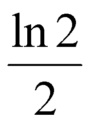 (approx. 0.347). However, the initial distribution of ions is not Gaussian and can be approximated better by a rectangular distribution, as also pointed out by the developers of the semi-empirical model.35 Thus, considering a rectangular initial distribution, the optimal value of β appears as
  (approx. 0.462). These values can be easily calculated using the second column of Table 1 and the relation
  (the latter value is to be obtained by calculating the FWHM of a Gaussian with the same variance as the uniform distribution whose width at the baseline equals tinj). The two above values of β are in good agreement with those obtained by May et al. employing the fitting procedure in their carefully executed study to characterize the performance of a commercially available DTIM-MS instrument.40 Experimentally determined β coefficients that are even smaller than the ideal value – obtained for very long gating times in the aforementioned study – are indicative of untimely depletion of the ion reserve. It means that the compartment storing the ions prior to injection (e.g. an ion funnel trap) becomes already empty before the gating time ends. In other words, the ion number density drops while the injection voltage is still applied and the initial distribution of ions does not follow the shape and width of the injection voltage pulse.
The two above-described variants are compatible with each other, one only needs to be careful when comparing β coefficients from different studies. They could be defined according to either of the two systems, meaning that suitable conversion between the scales might be required before comparing the performance of instruments.
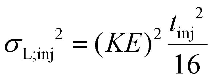
Even though tinj may be a parameter set by the operator of the IM-MS device, the third row of Table 1 makes it apparent that spatial variance depends on other instrumental parameters and on the nature of the analyte as well.66 The spatial outspread of the injected ion cloud also depends on the mobility of the ions, the drift voltage and the length of the mobility cell (the latter two determining together the electric field strength).
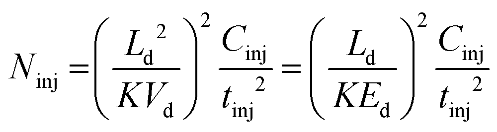 | (18) |
 | (19) |
Inferred from the variances of the initial ion distributions, the above equations show the limit of plate numbers and resolving power for the extrinsic contribution of the finite injection. Cinj is the appropriate constant depending on the density function describing the injection pulse profile (for a rectangular pulse, Cinj equals 12, as shown in Table 1).
It is apparent that Ninj and Rp;inj depend explicitly on Ld, representing the importance of the ion package size relative to the length of the drift cell. Furthermore, the limit of resolving power is inversely proportional to the drift voltage/electric field strength, in strong contrast to the effect of diffusion or Coulomb repulsion. This latter phenomenon leads to an important consequence regarding the apparent resolving power and its dependence on the drift voltage, namely that f(Vd) = Rp;app is not a monotonically increasing function. Instead, it has a maximum, corresponding to the operating condition where resolving power is the highest, while further increase in the field strength results in lower resolving power due to the increased contribution of the initial ion package size.31,39,40
Finally, it is important to point out that among all intrinsic and extrinsic sources of dispersion, the injection pulse-width is the only one where the corresponding theoretical plate and resolving power limits depend on pressure, because they depend on the absolute value of a single transport property. In other words, the implicit dependence of Ninj on p is due to its inverse proportionality to K2. Employing higher buffer gas pressure lowers the ion mobility, which consequently decreases σL;inj2 and increases td, Ninj and Rp;inj. As mentioned before, Ndiff does not depend on p at all, as the effects of D and K cancel out (the sum of their exponents is zero in eqn (5)–(7)). Thus, the positive influence of higher buffer gas pressures on the resolving power in IMS is largely due to its effect on the injection pulse-width and the higher drift voltages it enables.
In the model described above we assumed that the ions’ distribution follows exactly the injection voltage profile. In most cases a near-perfect rectangular voltage profile (step function) can be achieved to inject ions into the mobility cell, irrespective of the gating mechanism (Bradbury–Nielsen gate, ion funnel trap, etc.). However, it has been shown that the leading- and tailing edges of the ion density function do not follow accurately the shape of a step function, which may lead to deviations between theory and experimental data.35 Therefore, the importance of detailed simulations to obtain a more accurate picture (albeit at the cost of sacrificing generality) on ion injection should be emphasized. Such simulations can be performed considering the specific design of the instrument, as well as the mass-, mobility- and charge-distribution of the ions.
3.5. Extrinsic contributors II. Dispersion and separation after the mobility cell
In IM-MS, mass analysis and ion detection are spatially segregated from ion mobility separation, and take place in different compartments of the instrument. Therefore, ions require a finite time to reach the detector after having traversed the mobility cell. During this time, ion clouds continue expanding due to diffusion, Coulomb repulsion or other processes. Imperfections in ion transmission and distortions originating from electric field inhomogeneities in this region could deteriorate the performance of the instrument. Although they do not concern stand-alone IMS, the problems addressed in this section are all the more important in IM-MS. Post-cell dispersion in IM-MS, when not accompanied by mobility separation (e.g. transport in the high-vacuum region), is analogous to extra-column band broadening in HPLC, where solutes also require a finite time to reach the detector after their elution from the column.67–71 In an ion funnel, on the other hand, additional mobility separation takes place,72 making this situation similar to the serial coupling of multiple columns in chromatography.73,74 Although not to be confused, these two different cases of post-cell ion transport can be treated in an integrated manner, as shown in the present section.First, let us consider dispersion in an ideal ion funnel, where T, p and, consequently, the transport properties K and D have the same values as inside the drift cell. In this case, diffusional broadening can be expressed as below, by defining tfun as the time the ions spend in the funnel, and substituting into the Einstein equation (eqn (S1)†):
 | (20a) |
 | (20b) |
The equations above are completely analogous to eqn (5a) and (5b). As in a funnel the longitudinal motion of ions is driven by a DC field, tfun can be expressed using the length of this compartment and the corresponding voltage: Lfun and Vfun, respectively. Coulomb-driven dispersion can be addressed in an analogous way. When substituting tfun into eqn (8) (and eqn (S14)†), the variances appear as:
 | (21a) |
 | (21b) |
Variances associated with diffusion and Coulomb repulsion in the funnel are additive, their sum being the contribution of the funnel to the total dispersion (σfun2). As mentioned above, dispersion is not the only aspect of ion transport in a funnel. The separation of ions continues and it occurs with unaltered selectivity, i.e. the relative velocity difference of zones is the same as inside the drift cell. Thus, the residence time in this region (or the length of the funnel) needs to be accounted for when calculating the apparent separation efficiency. To explore this problem, let us borrow from the toolbox of chromatography.
In gas chromatography and HPLC the apparent effective plate number (Napp;chrom) that accounts for extra-column band broadening as well is given as:
 | (22) |
In eqn (21)tcol1, tcol2 and tec are the column- and extra-column residence times, respectively, their sum being the observed retention time (tr), while σt;col12, σt;col22 and σt;ec2 are the corresponding temporal variances. It is important to emphasize that the equation above is capable of handling any given number of columns and extra-column compartments. As the flow rate in chromatography is constant and bands move with constant volume velocity, temporal variances could be replaced by volume variances and the residence times could be substituted with their volume equivalents (retention volume, Vr, etc.). It is equivalent to expanding the numerator and the denominator with the volumetric flow rate. F is a dimensionless factor, defined as:
 | (23) |
Thus, F expresses the ratio of the nonseparative transport time (residence time in compartments where no separative transport takes place, in this case it equals tec) and the total runtime from injection to detection (here equals tr). Correcting with (1 − F)2 is mathematically equivalent to including only those compartments into the numerator where actual separative transport takes place, i.e. residence time in the columns. Although in the literature this factor is usually designated as R,75 we use the F notation to avoid confusion with resolving power (Rp).
In analogy to column chromatography, for IM-MS it can be written that:
 | (24) |
Here, Napp is the apparent effective plate number in DTIM-MS. The sum of the temporal variances that arise from injection, diffusion and Coulomb repulsion inside the drift cell is σt;cel1,2 while ta is the observed arrival time. The mobility cell and the funnel correspond to the columns (multiple drift cells could also be considered76). The residence time in the compartments where no mobility separation takes place (tns) is the analogue of the extra-column residence time (tec). The temporal variance associated with this region, σt;ns2, is the equivalent of σt;ec2. It can include dispersion in the low- and high-vacuum regions of IM-MS instruments, such as the ring-electrode or multipole ion guides. These are nontrivial to estimate and no attempt will be made here to explore them: when calculating the extra-cell dispersion, only contribution from the funnel will be considered. In IM-MS F appears as:
 | (25) |
For the instrument employed in this study, tns is the time spent in the low- and high-vacuum regions of the instrument between the funnel and the detector. As the relative velocity difference of ions does not reflect their mobility here, the length of these regions and the time spent here are not utilized for ion mobility separation. Whereas tfun can take up a significant portion of the arrival time, generally in the range of 5–25% in today's commercially available and custom-built devices, tns is generally less significant. The model given above to obtain the apparent effective separation efficiency is general: considering dispersion in every compartment, while accounting for migration only in those where actual separative transport takes place. Therefore, it can be adapted to any specific design (i.e. RF-confining drift cells), not only to instruments equipped with an exit funnel. This formalism proves to be very helpful when relating peak-to-peak resolution to the number of theoretical plates and selectivity, which will be explored in a subsequent publication.
 | (26) |
Here, σL1 and σL2 are the spatial standard deviations, while v1 and v2 are the zone velocities in the first and second compartment, respectively. The distances between the zones also expand or contract accordingly, meaning that it is not possible to improve the separation efficiency this way. To express the apparent plate number using spatial variances, one needs to incorporate this relation into the appropriate equations.
In the simplest case, the linear velocity of the ion clouds is constant across compartments, meaning that no velocity-correction is needed. If we also assume the funnel being the only post-cell compartment (also means that F is zero), the apparent plate number is given by:
 | (27) |
For eqn (27) to be true, the DC field needs to be the same in the two regions of the instrument (Ed = Efun). In this very specific case, the separation field can be considered uniform (if inhomogeneities of the electric field are not considered), and the exit funnel serves as the linear extension of the drift cell.77 A uniform separation field means that the local HETP is constant and does not vary from point to point or between compartments.
Even though the relative velocity difference of zones in an ideal exit funnel is the same as in the drift cell, the absolute velocities and the electric field strength are practically always different in the two compartments. Eqn (27) yields a correct solution when the zone velocities are equal, but gives systematically erroneous results when they are not. The larger the difference in the zone velocities, the larger the error appears. Thus, when the DC field and the velocities in the two compartments differ significantly (Ed ≠ Efun), a correction of eqn (27) is required according to eqn (26):
 | (28) |
This situation results in a nonuniform separation field where the local HETP varies between compartments, similarly to the case of serially coupled columns in chromatography.73 When the HETP is not constant, an apparent (not average) plate height can be defined to characterize the whole separation. For j compartments, the general solution can be given as the following, upon relating the velocity in each of the j regions (vi) to the drift velocity (vd):
 | (29) |
The general form of the apparent plate height can be expressed as:
 | (30) |
In eqn (29) the denominator contains the sum of the velocity-corrected effective (VCE) spatial variances, while the numerator is the sum of the velocity-corrected effective (VCE) separation lengths (left); this expression simplifies upon eliminating vd2 from the numerator and the denominator (middle), yielding the ratio of ta and the sum of the temporal variances (right) corrected with F, as expected. Eqn (28) and (29) also show that, in order to achieve the highest possible resolving power in IM-MS and utilize the separation potential of the exit funnel, one needs to carefully adjust the zone velocities in this post-cell compartment. Low ion velocities in the funnel mean that plenty of time is available for the ion clouds to spread in this compartment due to diffusion and space charge effects, and lead to large VCE spatial variances. On the other hand, very high zone velocities in the funnel might help prevent unwanted zone spreading, but the separation in this compartment will also be negligible as the VCE separation length of the funnel decreases. The following relations are true for the two VCE quantities:
| LVCE;i = tivd | (31a) |
| σL-VCE;i2 = σt;i2vd2 | (31b) |
L VCE and σL-VCE2 are directly related to the corresponding temporal quantities through the drift velocity, and not through the average velocity or the specific velocity of the ions in the individual compartments of the instrument. They express how broad the zones and how long the compartments would be in space if the zones were moving with vd in each compartment (with the temporal variance remaining unaltered). The overall voltage drop along the whole separation field could be conveniently used if the separation field was uniform. By introducing the VCE quantities, it becomes possible to handle nonuniform separation fields in a simple manner as well. Let us realize that the VCE length of the drift cell is the same as its actual length, and the spatial variances that are related to processes inside the mobility cell are also unaffected – only quantities associated with post-cell regions are modified to allow for an integrated treatment. It is also important to point out that – unlike the actual lengths – the sum of the VCE separation lengths is not constant: it is a function of the applied drift voltage. Therefore, HETPapp is related to Napp through the actual length that is independent of Vd (see eqn (30)).
3.6. Comparing plate-height models: analogies between different separation methods
Plate-height models are the most widespread models in the broad field of separation science, serving as a unified language across the techniques. They owe their popularity to their simplicity, predictive potential and their flexibility, i.e. to the fact that upon the satisfaction of a few criteria (nonlinear effects being weak and zones converging toward a Gaussian profile), plate-height models can be applied to virtually any differential migration method.Formal analogies between the plate-height model of linear DTIM-MS and that of column chromatography are apparent, with independently acting dispersion phenomena determining zone broadening in both techniques. Although the statistical framework (addition of variances) and figures of merit (N, HETP) are essentially the same, the underlying physical principles are of course fundamentally different. The main contributors to band broadening in column chromatography are eddy dispersion, axial diffusion and resistance to mass transfer.6,78,79 In DTIM-MS, on the other hand, axial diffusion, Coulomb repulsion, electric field inhomogeneities and the injection pulse-width were identified as major dispersion processes. By combining the effect of these phenomena, it is possible to formulate a plate-height equation similar to the Van Deemter equation in chromatography, with separate terms corresponding to each contributing factor (section 4.1, Fig. 2).
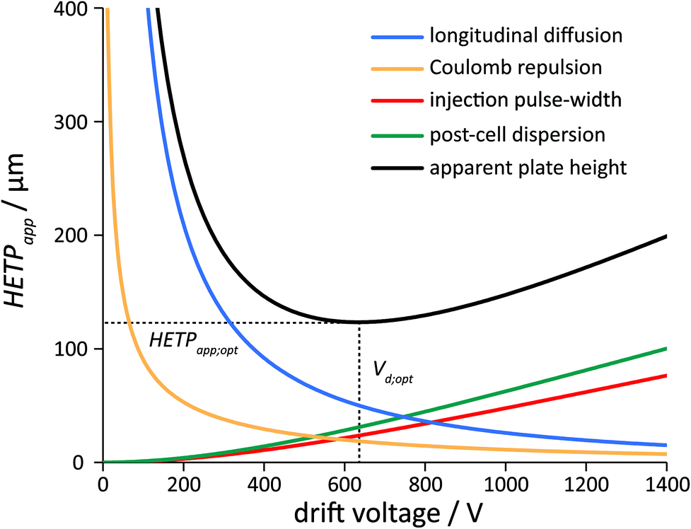 | ||
Fig. 2 Graphical representation of the plate-height equation in IM-MS. The apparent effective plate height (HETPapp) and the contribution of the various dispersion processes are highlighted with different colours, as indicated. Decreasing the drift voltage below the optimal value (Vd;opt) results in increased broadening and in decreased signal-to-noise ratio. Operating the instrument above Vd;opt leads to an improved S/N ratio in exchange of larger HETPapp.91 Note that Vd cannot be increased infinitely without generating discharges (practical limitation) or exceeding the low-field limit where the underlying equations break down (theoretical limitation of linear DTIMS). Calculations were performed employing eqn (35) and the following input parameters (identical to those used for the corresponding experiment, shown in Fig. 3): He buffer gas, p = 3 mbar, Ld = 805.5 mm, Lfun = 144 mm, T = 294.8 K, tinj = 150 μs, tfun = 1.627 ms and DTΩHe = 139 Å2 (trisaccharide Na+ adduct). Rectangular injection profile (Cinj = 12), ion clouds with a charge of Q = 100000e (CClmb =  , rectangular distribution) and a completely homogeneous electric field (θ = 1) were considered. , rectangular distribution) and a completely homogeneous electric field (θ = 1) were considered. | ||
Another aspect of DTIM-MS that has its analogue in chromatography is that of nonuniform separation fields, discussed in section 3.5.1. Although the origin of nonuniformity in DTIM-MS (changes in the electric field across compartments) are different from that in chromatography (gas compression effects and coupled columns), they both lead to changes in zone velocities and require analogous solutions.73
Plate-height models have also been established and employed for zone electrophoresis.14,80,81 As some dispersion processes found both in zone electrophoresis and ion mobility spectrometry act similarly, certain equations in the plate-height models of the two methods resemble each other, diffusion being a prominent example. In contrast to linear DTIM-MS, however, nonlinear effects are often so dominant in condensed phase electrophoretic systems that the validity of linear plate-height models may be limited.44–46
4. Results and discussion
4.1. Total peak broadening and the plate-height equation in ion mobility-mass spectrometry
Having addressed the various dispersion processes in IM-MS individually, in this section we aim to synthesize the findings to obtain a formula that is similar in nature to van Deemter's plate-height equation for chromatography. This equation may aid instrument design and development, as well as the optimization of measurement conditions to improve the performance of IM-MS separations. When multiple processes contribute to dispersion and broadening, the variances are additive. Therefore, the total variance generated during the whole IM-MS analysis – from injection to detection – can be expressed in the form below, using either temporal variances or spatial variances with velocity-correction. The variances σdiff2 and σClmb2 may also include θ to account for the effects of electric field inhomogeneities: | (32) |
It is important to mention at this point that in the macroscopic model presented in this study a single-species experiment was implicitly assumed, meaning that the effect of interconversion on peak widths was excluded. Although interconversion between different conformers or other isomeric species may influence the appearance of the ATDs, this phenomenon should not be confused with broadening due to physical processes. Therefore, when discussing their impact on peak shapes, one has to make a clear distinction between physical (dispersion due to diffusion, coulombic forces, etc.) and chemical (interconversion dynamics, ion-neutral reactions) processes, and treat them separately. The effect of the latter ones is addressed briefly as follows. The situation in ion mobility spectrometry is very similar to that in dynamic electrophoresis and dynamic chromatography.82–88 If interconversion takes place on a time-scale significantly faster than the time-scale of the separation, the peaks that would correspond to the separate conformers/isomers will merge into a single feature with no additional broadening.89,90 Fast-interconverting ions will drift with a velocity that is the weighted average of the drift velocities of the individual conformers/isomers. On the other hand, if the time-scale of interconversion is significantly longer than the time-scale of IMS analysis, the different conformers should be treated as distinct species that can be separated using IMS, provided their mobilities are different and the resolving power of our method is sufficiently high. Finally, if the time-scale of interconversion dynamics is comparable to the time-scale of separation, the coalescence of peaks will be incomplete. The aforementioned incomplete coalescence due to dynamic chemical phenomena, however, should not be confused with broadening due to physical processes.
Both the Van Deemter equation (based on a macroscopic view of the elution process) and the Giddings equation (based on a microscopic/stochastic theory of chromatography) describe band-broadening as a function of mobile phase velocity, expressing separation efficiency using plate heights.6,19 Plotting HETP as a function of the mobile phase velocity results in the well-known characteristic curves for chromatography, whose minima correspond to the conditions where the highest resolving power is achieved.79 The velocity of a band in chromatography (vband) is determined by the mobile phase linear velocity (vmobile) and the retention factor of the solute (k):
 | (33) |
The drift velocities in IMS are determined by the electric field strength and the ion mobility (vd = KEd = KVd/Ld). In this formal analogy Ed corresponds to vmobile, while K has a similar role to that of 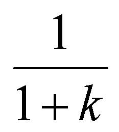 . Therefore, the resolving power and other figures of merit in IMS and IM-MS are often represented as a function of the electric field strength or, more conveniently, as a function of the drift voltage.
The total velocity-corrected effective spatial variance can be rewritten in the following simple form, highlighting the role of the drift voltage:
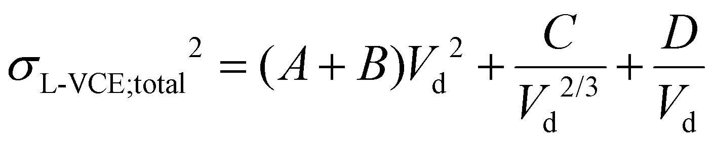 | (34) |

In the above formula the A-term corresponds to dispersion in the funnel, the fraction outside the square brackets accounting for the velocity-correction (employing the relation v = KV/L). The dependence of the funnel's contribution on Vd does not mean that the actual spatial or temporal variances associated with this compartment are influenced by the applied drift voltage. It only means that its relative contribution increases with decreasing drift times, as its contribution is weighted with the factor vd2/vfun2. The B-term reflects the influence of the injection pulse-width, while the C- and D-terms are associated with the contribution of Coulomb repulsion and diffusion inside the drift cell, respectively. In the instrument employed in the present study, the post-cell residence time mostly represents the time spent in the funnel, and the funnel is assumed to be the only post-cell compartment in the calculations. This simplification means that tns and F equal zero and ta = td + tfun. The drawback of eqn (34) is that the velocity corrected effective length of the separation field also depends on Vd and the minimum of this function does not correspond to the point where the resolving power is the highest. Therefore, it is more meaningful to plot HETP as the function of Vd.
 | (35) |
Eqn (35) is the apparent effective plate height in DTIM-MS, the analogue of the plate-height equations in chromatography and the central expression of the plate-height model presented in this study. The function above shows the contribution of the individual dispersion processes in an additive form, as represented in Fig. 2. Analogously to HETPapp, the apparent effective plate number and -resolving power can be expressed as:
 | (36) |
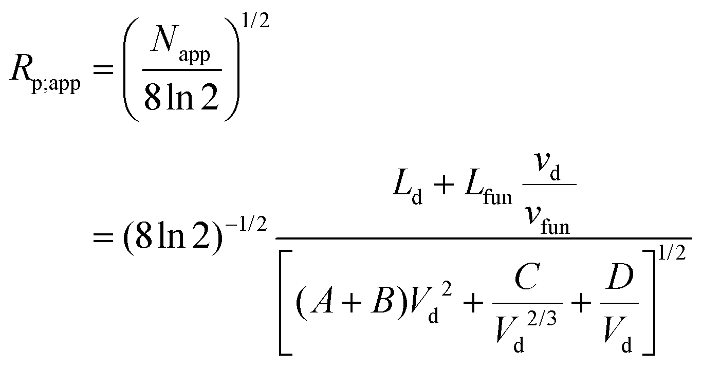 | (37) |
HETPapp, Napp and Rp;app can be calculated from each other with ease. In case of stand-alone IMS eqn (34)–(37) simplify significantly, as Lfun is zero and the separation field becomes uniform. The aforementioned simplified equations can be found in the ESI, section S4.† Section S4 also contains a straightforward method to find the plate-height function's minimum where separation is optimal (Vd;opt and HETPopt), and the expression of HETPapp, Napp and Rp;app using temporal variances. In the IMS and IM-MS communities, resolving power is generally favored over theoretical plates and plate height, probably due to its attractive feature of being directly proportional to peak-to-peak resolution. Therefore, to make the results and findings of this study comparable to those present in the literature, the next section utilizes resolving power as a measure of separation efficiency.
4.2. Comparison of theory and experiments: evaluation of the plate-height model
To evaluate the accuracy of the plate-height model and its capability to predict the effect of different experimental parameters and the nature of the analyte on the resolving power in IM-MS, a series of measurements were performed using a custom-built instrument (see Fig. 1 and section 2.2). The buffer gas pressure, the injection pulse-width and the collision cross section of the investigated ions were varied in a systematic manner, followed by the comparison of the experimentally obtained data and the results of calculations, as presented in Fig. 3. | ||
| Fig. 3 Resolving power in IM-MS – experiment vs. theory. The effect of (A) the buffer gas pressure, (B) the injection pulse-width and (C) the collision cross section of the ions on the apparent effective resolving power (Rp;app) is highlighted. Experiments were performed in positive ion mode on a custom-built DTIM-MS instrument (Ld = 805.5 mm, Lfun = 144 mm) with He as buffer gas at ambient temperature (T = 295.0 ± 0.2 K). The following measurement conditions were used as a starting point with the corresponding curve presented in every graph (red, yellow and blue trace in A, B and C, respectively): p = 3 mbar, tinj = 150 μs and DTΩHe = 139 Å2 (trisaccharide Na+ adduct). Each of the three aforementioned experimental parameters was varied systematically as follows. (A) Buffer gas pressure varied in three steps: 3 mbar, 4 mbar and 5 mbar. (B) Injection pulse-width varied in three steps: 50 μs, 100 μs and 150 μs. (C) Collision cross section (influencing the mobility of the ions) varied in three steps: DTΩHe = 74 Å2 (protonated 12-crown-4), 139 Å2 (trisaccharide Na+ adduct) and 270 Å2 (TBAI trimer). Calculations were performed according to eqn (37), considering a rectangular injection profile (Cinj = 12), ion clouds with a charge of Q = 100000e (CClmb = 1/3, continuous uniform distribution) and a completely homogeneous electric field (θ = 1). | ||
In all three cases the plate-height model exhibits satisfactory agreement with experimental results despite its simplicity, being able to reproduce and predict the observed trends and the influence of the various parameters on the resolving power of IM-MS. Although the buffer gas pressure is not present explicitly in eqn (37), the harmony between theory and experiment makes the implicit dependence evident. Fig. 3c highlights that the behavior of distinct ions in IM-MS might be very different, even under the same experimental conditions. This underlines the importance of method optimization in applications where analytes span over a wide range of mobility, such as in the various omics fields. The slightly different behavior of the protonated 12-crown-4 ion (DTΩHe = 74 Å2) that leads to suboptimal agreement is arguably due to the exceptionally high mobility of this ion under the conditions employed. The trapping entrance funnel storing the ions prior to injection may become already empty before the gating time ends, and the width of the ion packet does not follow the width of the injection pulse, shifting the experimentally obtained curve's maximum toward higher Vd values. Furthermore, in Fig. 3c the experimentally obtained trace corresponding to the aforementioned species does not overlap at low drift voltages with the traces corresponding to the two other ions. Such lack of overlap in the diffusion dominated region might be indicative of additional peak broadening due to dynamic chemical phenomena.
Although agreement between experiment and theory is satisfactory, it cannot be considered perfect. The potential sources of the slight discrepancy (overestimation of the resolving power by the plate-height model) can be manifold. Additional broadening due to the finite speed of amplifiers and the finite response time of the detector, underestimation of dispersion outside the mobility cell (the contribution of the low- and high-vacuum regions was not considered) can all contribute to the difference. Imperfect description of the initial spread of the ion clouds by the simple equations presented in section 3.4 is another plausible reason. It also explains the moderate, but systematic shift of the experimentally obtained curves’ maxima (Vd;opt) to lower values along the x-axis (except for the crown ether, as discussed above). It is in accordance with the fact that the values determined for the β coefficient in the semi-empirical model are often larger than ideal.35 These findings again underline the importance of ion trajectory simulations to characterize the injection mechanism of a given instrument. The equivalent of Fig. 3 using plate heights instead of resolving power, as well as an analogous comparative analysis with tetrabutylammonium iodide ions can be found in the ESI, sections S5.† In contrary to the semi-empirical resolving power theory, the plate-height model is a predictive concept, as it is based on first principles rather than on a fitting-procedure. Having tested its accuracy, the next section explores the predictive power of the model.
4.3. Predictive potential of the plate-height model
In the present section, the impact of key experimental variables and analyte characteristics (such as the collision cross section or the charge-state of the ions) on resolving power in IM-MS are highlighted through four examples. For the calculations, hypothetical analytes were used to emphasize the generality of the plate-height model and its applicability to ions spanning over a wide range of size and charge. Calculations were performed using conditions generally applied or realistically achievable with today's commercially available or research-grade instruments. The electric field in the funnel was held constant at 10 V cm−1. For the calculations, the dimensions of the custom-built DTIM-MS instrument (described in the Experimental section) were considered. Dispersion in regions following the exit funnel was neglected. | ||
Fig. 4 Influence of the injection pulse-width on the plate height and resolving power in IM-MS. (A) The apparent effective plate height (HETPapp) and (B) the apparent effective resolving power (Rp;app) as a function of the drift voltage. Different colours correspond to different tinj values as indicated. The black dashed lines correspond to an infinitesimally narrow injection pulse, i.e. a Dirac delta-function. Calculations were performed according to eqn (35) and (37), respectively, with the same input parameters: He buffer gas, p = 4 mbar, T = 298.15 K (25 °C), Ld = 805.5 mm, Lfun = 144 mm, DTΩHe = 200 Å2, m = 1000 u, z = 1. Injection pulse-width was varied from 25 μs to 250 μs in 10 equidistant steps as highlighted in the figure. The electric field strength in the funnel was held constant at 10 V cm−1. Rectangular injection profile (Cinj = 12), ion clouds with a charge of Q = 100000e (CClmb = 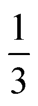 , continuous uniform distribution) and a completely homogeneous electric field (θ = 1) were considered. , continuous uniform distribution) and a completely homogeneous electric field (θ = 1) were considered. | ||
 | ||
Fig. 5 Influence of the buffer gas pressure on the plate height and resolving power in IM-MS. (A) The apparent effective plate height (HETPapp) and (B) the apparent effective resolving power (Rp;app) as a function of the drift voltage. Different colours correspond to different pressure values as indicated. The black dashed lines (identical to those in Fig. 4) correspond to the fundamental limit of resolving power and plate heights, determined by diffusion and Coulomb repulsion. This limit is completely independent of the applied pressure. Calculations were performed according to eqn (35) and (37), respectively, with the same input parameters: He buffer gas, T = 298.15 K (25 °C), tinj = 150 μs, Ld = 805.5 mm, Lfun = 144 mm, DTΩHe = 200 Å2, m = 1000 u, z = 1. Pressure was varied from 2.5 mbar to 7 mbar in 10 equidistant steps as highlighted in the figure. The electric field strength in the funnel was held constant at 10 V cm−1. Rectangular injection profile (Cinj = 12), ion clouds with a charge of Q = 100000e (CClmb =  , continuous uniform distribution) and a completely homogeneous electric field (θ = 1) were considered. , continuous uniform distribution) and a completely homogeneous electric field (θ = 1) were considered. | ||
The functions corresponding to higher pressures start deviating from this fundamental limit at higher drift voltages. This phenomenon is completely analogous to that observed upon decreasing the injection pulse-width, as the effect of increasing p and decreasing tinj is the same: lower B-terms meaning narrower initial ion packets in space. Thus, Rp;app does not grow infinitely with increasing pressure at a given drift voltage. It can only increase until the limit set by the pressure-independent contributors is reached, i.e. where the finite size of the injected ion packet is negligible. It is demonstrated by the overlapping regions of the curves at low drift voltages, where the initial spread of the ion cloud is still insignificant, with diffusion and space charge effects being dominant in determining zone spreading. In conclusion, the buffer gas pressure exerts its effect on resolving power mostly through influencing the initial spatial spread of the ion cloud. The same conclusions can be drawn by analyzing the functions showing HETPapp as well, keeping in mind that lower values correspond to more efficient separations. Although not shown in Fig. 5, higher pressures inside the mobility cell also enable the application of higher drift voltages by reducing the probability of discharges and expanding the low-field limit toward higher drift fields.
 | ||
Fig. 6 Influence of the ions’ collision cross section on the plate height and resolving power in IM-MS. (A) The apparent effective plate height (HETPapp) and (B) the apparent effective resolving power (Rp;app) as a function of the drift voltage. Different colours correspond to different DTΩHe values as indicated. Calculations were performed according to eqn (35) and (37), respectively, with the same input parameters: He buffer gas, p = 4 mbar, T = 298.15 K (25 °C), tinj = 150 μs, Ld = 805.5 mm, Lfun = 144 mm, z = 1. DTΩHe was varied from 50 Å2 to 500 Å2 in 10 equidistant steps as highlighted in the figure. Although the influence of m on K is negligible in these cases, the masses of the ions were also varied mimicking an isotropic growth pattern to achieve more realistic conditions: m = 150 u, 350 u, 650 u, 1000 u, 1400 u, 1850 u, 2350 u, 2900 u, 3500 u and 4150 u (in the order of increasing collision cross sections). The electric field strength in the funnel was held constant at 10 V cm−1. Rectangular injection profile (Cinj = 12), ion clouds with a charge of Q = 100000e (CClmb =  , continuous uniform distribution) and a completely homogeneous electric field (θ = 1) were considered. , continuous uniform distribution) and a completely homogeneous electric field (θ = 1) were considered. | ||
 | ||
Fig. 7 Influence of the ions’ charge-state on the plate height and resolving power in IM-MS. (A) The apparent effective plate height (HETPapp) and (B) the apparent effective resolving power (Rp;app) as a function of the drift voltage. Different colours correspond to different charge-states as indicated. Calculations were performed according to eqn (35) and (37), respectively, with the same input parameters: He buffer gas, p = 4 mbar, T = 298.15 K (25 °C), tinj = 150 μs, Ld = 805.5 mm, Lfun = 144 mm, DTΩHe = 500 Å2 and m = 4150 u. The charge-state was varied from z = 1 to 10 as highlighted in the figure (the polarity being irrelevant). The electric field strength in the funnel was held constant at 10 V cm−1. Rectangular injection profile (Cinj = 12) and a completely homogeneous electric field (θ = 1) were considered. The total number of ions was varied so that the charge of the ion clouds be fixed at Q = 100000e (CClmb =  , continuous uniform distribution). , continuous uniform distribution). | ||
Fig. 6 highlights the influence of the collision cross section on HETPapp and Rp;app, considering a set of singly-charged ions with DTΩHe ranging from 50 Å2 to 500 Å2. Because dispersion due to diffusion and coulombic forces depend on the ratio and not on the absolute value of transport properties, terms A, C and D are unaffected by a change in the collision cross section. The B-term – corresponding to the initial ion cloud size – is the only among the four that depends on the actual absolute value of a single transport property: K. Therefore, Vd;opt and Rp;app;opt increase monotonously for larger ions within a given charge-state.
Fig. 7 shows how the apparent effective plate height and resolving power change across charge-states in the case when the collision cross section is kept constant. In order to examine the impact of mobility independently from space charge effects, the total charge of the ion clouds was fixed at 100000e. The appearance of Fig. 7 is strikingly different from that of Fig. 4–6. First, curves corresponding to ions with different charge-states do not overlap at low Vd. The lack of overlap is the consequence of the fact that ions of different charge-states are characterized by different D-terms. Unlike tinj, p or Ω, the charge-state of ions has as an influence on the diffusion limit of resolving power as the K/D ratio is a function of z. A second apparent difference is that instead of running parallel, the curves tend to intersect each other at certain drift voltages. Besides having a strong effect on the D-term (and also on the A-term as it incorporates diffusion in the funnel), z influences the B-term and the initial spread of the ion packet too. As a consequence, Vd;opt decreases systematically when the charge-state increases. The intersections stem from the simultaneous influence of the aforementioned antagonistic effects: decreasing D- and A-terms (the total charge of the ion cloud, i.e. the C-term is kept constant) and an increasing B-term as the charge-state increases. As the drift voltage is increased, the trace of an ion with lower charge-state intersects, then surpasses the curves corresponding to highly-charged species, when the beneficial effect of a narrower initial ion packet balances and – ultimately – overcomes the detrimental effect of increased diffusional broadening. The differences between the appearance of Fig. 7 and 4–6 stem from the fact that the ions’ charge-state is the only factor that has an influence on multiple terms, unlike tinj, p and Ω, which only affect the B-term.
Fig. 7 also shows the dependence of the maximally achievable resolving power on z in IM-MS. First, the maximum increases upon moving from z = 10 down to the doubly-charged species, then it drops significantly as z is further decreased from 2 to 1. It needs to be mentioned that under different operating conditions or considering smaller/larger ions, the trend may be different. The dependence of the maximum of Rp;app on the charge-state of ions is the consequence of Coulomb repulsion and the nonuniformity of the separation field in DTIM-MS. Note that the electric field strength in the exit funnel is fixed at a defined value, which influences the achievable resolving power of distinct ions differently. Interestingly, in stand-alone DTIMS, where the separation field is uniform, the maximally achievable resolving power does not depend on the charge-state of the ions if space charge effects are also neglected (see ESI, section S4, eqn (S28)–(30),† and a theoretical study by Kirk et al.39).
Finally, both Fig. 6 and 7 show the difficulties posed by samples containing analytes that span over a wide mobility-range. Optimizing the ion mobility separation to achieve sufficient resolving power for as many ions as possible is an important aspect of targeted and nontargeted omic analyses utilizing IM-MS.33,97–100
5. Conclusion and outlook
A plate-height model of IM-MS was developed and verified against a comprehensive set of experiments. This first-principles analytical model is based on the linear addition of variances that correspond to independently acting dispersion processes, in contrast to the FWHM-centered approaches presented so far in IMS literature. Using the variance-based concept, optimal values of the β coefficient in the semi-empirical resolving power theory could be rationalized (section 3.4). Moreover, the introduction of velocity-corrected effective spatial variances offers a straightforward way to describe separations in nonuniform fields, for example in the presence of ion funnels (section 3.5.1). To the best of our knowledge, this is the first general solution provided for the aforementioned problem in IM-MS.In the plate-height equation of DTIM-MS, four different integrated terms were established and rendered to the individual dispersion processes that determine the resolving power of the technique (see eqn (34)). This simple and concise formalism was conceived in analogy to the traditional A-, B- and C-terms in the Van Deemter equation for chromatography. Table 2 provides a brief overview of the most important aspects of the dispersion processes, described within the formalism of the plate-height model to show the corresponding integrated terms. The effect of the drift voltage on zone spreading, the role of transport properties and the influence of the most important instrumental parameters and analyte characteristics are highlighted. These also reveal the possibilities to minimize dispersion and maximize resolving power.
| Post-cell dispersion | Injection pulse-width | Coulomb repulsion | Longitudinal diffusion | |
|---|---|---|---|---|
| Corresponding integrated term | A-term | B-term | C-term | D-term |
| Dependence of σL-VCE2 on drift voltage | V d 2 | V d 2 | V d −2/3 | V d −1 |
| Related transport properties | Ratio of  and ratio of and ratio of  |
Absolute value of K | Ratio of  (cancels out) (cancels out) |
Ratio of  |
| Main influencing factors | v d/vfun – ratio of ion velocities in the drift cell and the exit funnel | t inj – injection time | Q – total charge of the ion cloud | T – buffer gas temperature |
| L d – length of the mobility cell | z – charge-state of ions | |||
| K – mobility of ions (p, T, z, Ω) |
In summary, the plate-height model can be easily implemented in spreadsheets, allowing for the calculation of zone spreading without ion trajectory simulations and the solution of nonlinear differential equations using numerical methods. Besides its simplicity, it offers a suitable nomenclature and a range of useful definitions and metrics – established originally for chromatography – to describe IMS and IM-MS separations, and to compare them to other separation techniques. Elements of the aforementioned toolbox, such as peak-to-peak resolution or peak capacity, will be addressed in subsequent studies, extending the plate-height concept for IM-MS.
Conflicts of interest
The authors declare no competing financial interest.Acknowledgements
The authors gratefully acknowledge financial support from the Freie Universität Berlin and the Max Planck Society. This research was funded by the German Research Foundation (FOR2177/P02). Open Access funding provided by the Max Planck Society.References
- W. A. Peters, Ind. Eng. Chem., 1923, 15, 402–403 CrossRef CAS.
- A. J. Martin and R. L. Synge, Biochem. J., 1941, 35, 1358–1368 CrossRef CAS PubMed.
- E. Glueckauf, Trans. Faraday Soc., 1955, 51, 34–44 RSC.
- A. S. Said, AIChE J., 1956, 2, 477–481 CrossRef CAS.
- L. Lapidus and N. R. Amundson, J. Phys. Chem., 1952, 56, 984–988 CrossRef CAS.
- J. J. van Deemter, F. J. Zuiderweg and A. Klinkenberg, Chem. Eng. Sci., 1995, 50, 3869–3882 CrossRef CAS.
- J. C. Giddings and H. Eyring, J. Phys. Chem., 1955, 59, 416–421 CrossRef CAS.
- J. C. Giddings, J. Chem. Phys., 1957, 26, 169–173 CrossRef CAS.
- D. A. McQuarrie, J. Chem. Phys., 1963, 38, 437–445 CrossRef CAS.
- F. Dondi and M. Remelli, J. Phys. Chem., 1986, 90, 1885–1891 CrossRef CAS.
- A. Cavazzini, M. Remelli, F. Dondi and A. Felinger, Anal. Chem., 1999, 71, 3453–3462 CrossRef CAS.
- F. Dondi, A. Cavazzini and L. Pasti, J. Chromatogr. A, 2006, 1126, 257–267 CrossRef CAS PubMed.
- L. D. C. Bishop and C. F. Landes, Acc. Chem. Res., 2018, 51, 2247–2254 CrossRef CAS PubMed.
- J. C. Giddings, Sep. Sci., 1969, 4, 181–189 CAS.
- J. C. Giddings, Unified Separation Science, John Wiley & Sons, Inc., New York, 1991 Search PubMed.
- C. H. Dilks Jr., H. J. Stoklosa, J. J. Kirkland and W. W. Yau, J. Chromatogr. Sci., 1977, 15, 303–316 Search PubMed.
- W. E. Barber and P. W. Carr, Anal. Chem., 1981, 53, 1939–1942 CrossRef CAS.
- J. P. Foley and J. G. Dorsey, Anal. Chem., 1983, 55, 730–737 CrossRef CAS.
- J. C. Giddings, Dynamics of chromatography, Marcel Dekker, New York, 1st edn, 1965 Search PubMed.
- M. Bonamente, Statistics and Analysis of Scientific Data, Springer, New York, 2nd edn, 2017 Search PubMed.
- S. Warnke, A Gas-Phase Approach to Biomolecular Structure: Combining Ion Mobility-Mass Spectrometry with Spectroscopy, Freie Universität, Berlin, 2015 Search PubMed.
- P. R. Kemper, N. F. Dupuis and M. T. Bowers, Int. J. Mass Spectrom., 2009, 287, 46–57 CrossRef CAS.
- H. E. Revercomb and E. A. Mason, Anal. Chem., 1975, 47, 970–983 CrossRef CAS.
- A. B. Kanu, M. M. Gribb and H. H. Hill, Anal. Chem., 2008, 80, 6610–6619 CrossRef CAS PubMed.
- M. A. Ewing, M. S. Glover and D. E. Clemmer, J. Chromatogr. A, 2016, 1439, 3–25 CrossRef CAS PubMed.
- A. T. Kirk and S. Zimmermann, Int. J. Ion Mobility Spectrom., 2015, 18, 17–22 CrossRef CAS.
- J. C. Giddings, J. Chromatogr. A, 1989, 480, 21–33 CrossRef CAS PubMed.
- E. R. Brocker, S. E. Anderson, B. H. Northrop, P. J. Stang and M. T. Bowers, J. Am. Chem. Soc., 2010, 132, 13486–13494 CrossRef CAS PubMed.
- J. C. May and D. H. Russell, J. Am. Soc. Mass Spectrom., 2011, 22, 1134 CrossRef CAS PubMed.
- J. Ujma, K. Giles, M. Morris and P. E. Barran, Anal. Chem., 2016, 88, 9469–9478 CrossRef CAS PubMed.
- S. Rokushika, H. Hatano, M. A. Baim and H. H. Hill, Anal. Chem., 1985, 57, 1902–1907 CrossRef CAS.
- K. L. Davidson and M. F. Bush, Anal. Chem., 2017, 89, 2017–2023 CrossRef CAS PubMed.
- V. D'Atri, T. Causon, O. Hernandez-Alba, A. Mutabazi, J.-L. Veuthey, S. Cianferani and D. Guillarme, J. Sep. Sci., 2017, 41, 20–67 CrossRef PubMed.
- P. Watts and A. Wilders, Int. J. Mass Spectrom. Ion Processes, 1992, 112, 179–190 CrossRef CAS.
- W. F. Siems, C. Wu, E. E. Tarver, H. H. J. Hill, P. R. Larsen and D. G. McMinn, Anal. Chem., 1994, 66, 4195–4201 CrossRef CAS.
- G. E. Spangler, Int. J. Mass Spectrom., 2002, 220, 399–418 CrossRef CAS.
- E. J. Davis, P. Dwivedi, M. Tam, W. F. Siems and H. H. Hill, Anal. Chem., 2009, 81, 3270–3275 CrossRef CAS PubMed.
- A. T. Kirk, M. Allers, P. Cochems, J. Langejuergen and S. Zimmermann, Analyst, 2013, 138, 5200–5207 RSC.
- A. T. Kirk, K. Bakes and S. Zimmermann, Int. J. Ion Mobility Spectrom., 2017, 20, 105–109 CrossRef CAS.
- J. C. May, J. N. Dodds, R. T. Kurulugama, G. C. Stafford, J. C. Fjeldsted and J. A. McLean, Analyst, 2015, 140, 6824–6833 RSC.
- T. J. Causon and S. Hann, J. Chromatogr. A, 2015, 1416, 47–56 CrossRef CAS PubMed.
- V. Hruška and B. Gaš, Electrophoresis, 2007, 28, 3–14 CrossRef PubMed.
- F. Kohlrausch, Ann. Phys., 1897, 298, 209–239 CrossRef.
- F. E. P. Mikkers, F. M. Everaerts and T. P. E. M. Verheggen, J. Chromatogr. A, 1979, 169, 1–10 CrossRef CAS.
- M. Bier, O. A. Palusinski, R. A. Mosher and D. A. Saville, Science, 1983, 219, 1281–1287 CrossRef CAS PubMed.
- B. Gaš, M. Štědrý and E. Kenndler, Electrophoresis, 1997, 18, 2123–2133 CrossRef PubMed.
- M. Dvořák, P. Dubský, M. Dovhunová and B. Gaš, Electrophoresis, 2019, 40, 668–682 CrossRef PubMed.
- H. Poppe, Anal. Chem., 1992, 64, 1908–1919 CrossRef CAS.
- F. E. P. Mikkers, Anal. Chem., 1999, 71, 522–533 CrossRef CAS.
- P. C. Haarhoff and H. J. Van der Linde, Anal. Chem., 1966, 38, 573–582 CrossRef CAS.
- G. L. Erny, E. T. Bergström, D. M. Goodall and S. Grieb, Anal. Chem., 2001, 73, 4862–4872 CrossRef CAS PubMed.
- G. L. Erny, E. T. Bergström and D. M. Goodall, J. Chromatogr. A, 2002, 959, 229–239 CrossRef CAS PubMed.
- G. E. Spangler, Anal. Chem., 1992, 64, 1312 CrossRef CAS.
- J. Xu, W. B. Whitten and J. M. Ramsey, Anal. Chem., 2000, 72, 5787–5791 CrossRef CAS PubMed.
- A. V. Mariano, W. Su and S. K. Guharay, Anal. Chem., 2009, 81, 3385–3391 CrossRef CAS PubMed.
- A. V. Tolmachev, B. H. Clowers, M. E. Belov and R. D. Smith, Anal. Chem., 2009, 81, 4778–4787 CrossRef CAS PubMed.
- G. E. Spangler, Anal. Chem., 2010, 82, 8052–8059 CrossRef CAS PubMed.
- M. Levin, A. Krisilov, B. Zon and G. Eiceman, Int. J. Ion Mobility Spectrom., 2014, 17, 73–77 CrossRef CAS.
- B. C. Hauck, W. F. Siems, C. S. Harden, V. M. McHugh and H. H. Hill, Int. J. Ion Mobility Spectrom., 2017, 20, 57–66 CrossRef CAS.
- G. E. Spangler and C. I. Collins, Anal. Chem., 1975, 47, 403–407 CrossRef CAS.
- E. A. Mason and H. W. Schamp, Ann. Phys., 1958, 4, 233–270 CAS.
- E. A. Mason and E. W. McDaniel, Transport Properties of Ions in Gases, John Wiley & Sons, Inc., New York, 1988 Search PubMed.
- L. A. Viehland, Gaseous Ion Mobility, Diffusion, and Reaction, Springer, 1st edn, 2018 Search PubMed.
- X. Huang, W. F. Coleman and R. N. Zare, J. Chromatogr. A, 1989, 480, 95–110 CrossRef CAS.
- A. C. Sanchez, J. A. Anspach and T. Farkas, J. Chromatogr. A, 2012, 1228, 338–348 CrossRef CAS PubMed.
- I. K. Webb, S. V. B. Garimella, A. V. Tolmachev, T.-C. Chen, X. Zhang, R. V. Norheim, S. A. Prost, B. LaMarche, G. A. Anderson, Y. M. Ibrahim and R. D. Smith, Anal. Chem., 2014, 86, 9169–9176 CrossRef CAS PubMed.
- F. Gritti, A. Felinger and G. Guiochon, J. Chromatogr. A, 2006, 1136, 57–72 CrossRef CAS PubMed.
- F. Gritti and G. Guiochon, J. Chromatogr. A, 2010, 1217, 7677–7689 CrossRef CAS PubMed.
- F. Gritti and G. Guiochon, J. Chromatogr. A, 2014, 1327, 49–56 CrossRef CAS.
- S. Fekete and J. Fekete, J. Chromatogr. A, 2011, 1218, 5286–5291 CrossRef CAS PubMed.
- K. Vanderlinden, K. Broeckhoven, Y. Vanderheyden and G. Desmet, J. Chromatogr. A, 2016, 1442, 73–82 CrossRef CAS PubMed.
- K. Tang, A. A. Shvartsburg, H.-N. Lee, D. C. Prior, M. A. Buschbach, F. Li, A. V. Tolmachev, G. A. Anderson and R. D. Smith, Anal. Chem., 2005, 77, 3330–3339 CrossRef CAS PubMed.
- J. C. Giddings, Anal. Chem., 1963, 35, 353–356 CrossRef CAS.
- O. Guiochon and J. E. N. Gutierrez, J. Chromatogr. A, 1987, 406, 3–10 CrossRef.
- J. C. Giddings, J. Chromatogr. Sci., 1964, 2, 167–169 CrossRef CAS.
- S. L. Koeniger, S. I. Merenbloom, S. J. Valentine, M. F. Jarrold, H. R. Udseth, R. D. Smith and D. E. Clemmer, Anal. Chem., 2006, 78, 4161–4174 CrossRef CAS PubMed.
- E. S. Baker, B. H. Clowers, F. Li, K. Tang, A. V. Tolmachev, D. C. Prior, M. E. Belov and R. D. Smith, J. Am. Soc. Mass Spectrom., 2007, 18, 1176–1187 CrossRef CAS PubMed.
- J. C. Giddings and K. L. Mallik, Anal. Chem., 1966, 38, 997–1000 CrossRef CAS.
- Liquid Chromatography: Fundamentals and Instrumentation, ed. S. Fanali, P. Haddad, C. Poole, P. Schoenmakers and D. Lloyd, Elsevier, 1st edn, 2013 Search PubMed.
- J. W. Jorgenson and K. D. Lukacs, Anal. Chem., 1981, 53, 1298–1302 CrossRef CAS.
- S. Hjertén, Electrophoresis, 1990, 11, 665–690 CrossRef PubMed.
- J. Veciana and M. I. Crespo, Angew. Chem., Int. Ed. Engl., 1991, 30, 74–76 CrossRef.
- O. Trapp, G. Schoetz and V. Schurig, Chirality, 2001, 13, 403–414 CrossRef CAS PubMed.
- J. Krupcik, P. Oswald, P. Májek, P. Sandra and D. W. Armstrong, J. Chromatogr. A, 2003, 1000, 779–800 CrossRef CAS PubMed.
- C. Wolf, Chem. Soc. Rev., 2005, 34, 595–608 RSC.
- O. Trapp, Anal. Chem., 2006, 78, 189–198 CrossRef CAS PubMed.
- L. Pasti, A. Cavazzini, M. Nassi and F. Dondi, J. Chromatogr. A, 2010, 1217, 1000–1009 CrossRef CAS.
- A. Sepsey, D. R. Németh, G. Németh and A. Felinger, J. Chromatogr. A, 2018, 1564, 155–162 CrossRef CAS PubMed.
- B. S. Kinnear, M. R. Hartings and M. F. Jarrold, J. Am. Chem. Soc., 2002, 124, 4422–4431 CrossRef CAS PubMed.
- S. Poyer, C. Comby-Zerbino, C. M. Choi, L. MacAleese, C. Deo, N. Bogliotti, J. Xie, J.-Y. Salpin, P. Dugourd and F. Chirot, Anal. Chem., 2017, 89, 4230–4237 CrossRef CAS PubMed.
- A. T. Kirk and S. Zimmermann, Int. J. Ion Mobility Spectrom., 2015, 18, 129–135 CrossRef.
- A. T. Kirk, D. Grube, T. Kobelt, C. Wendt and S. Zimmermann, Anal. Chem., 2018, 90, 5603–5611 CrossRef CAS PubMed.
- L. Deng, Y. M. Ibrahim, A. M. Hamid, S. V. B. Garimella, I. K. Webb, X. Zheng, S. A. Prost, J. A. Sandoval, R. V. Norheim, G. A. Anderson, A. V. Tolmachev, E. S. Baker and R. D. Smith, Anal. Chem., 2016, 88, 8957–8964 CrossRef CAS PubMed.
- L. Deng, I. K. Webb, S. V. B. Garimella, A. M. Hamid, X. Zheng, R. V. Norheim, S. A. Prost, G. A. Anderson, J. A. Sandoval, E. S. Baker, Y. M. Ibrahim and R. D. Smith, Anal. Chem., 2017, 89, 4628–4634 CrossRef CAS PubMed.
- S. Warnke, A. Ben Faleh, R. P. Pellegrinelli, N. Yalovenko and T. R. Rizzo, Faraday Discuss., 2019, 217, 114–125 RSC.
- A. T. Kirk, C.-R. Raddatz and S. Zimmermann, Anal. Chem., 2017, 89, 1509–1515 CrossRef CAS PubMed.
- J. C. May, C. R. Goodwin, N. M. Lareau, K. L. Leaptrot, C. B. Morris, R. T. Kurulugama, A. Mordehai, C. Klein, W. Barry, E. Darland, G. Overney, K. Imatani, G. C. Stafford, J. C. Fjeldsted and J. A. McLean, Anal. Chem., 2014, 86, 2107–2116 CrossRef CAS PubMed.
- X. Zheng, R. Wojcik, X. Zhang, Y. M. Ibrahim, K. E. Burnum-Johnson, D. J. Orton, M. E. Monroe, R. J. Moore, R. D. Smith and E. S. Baker, Annu. Rev. Anal. Chem., 2017, 10, 71–92 CrossRef CAS PubMed.
- T. Mairinger, T. J. Causon and S. Hann, Curr. Opin. Chem. Biol., 2018, 42, 9–15 CrossRef CAS PubMed.
- K. E. Burnum-Johnson, X. Zheng, J. N. Dodds, J. Ash, D. Fourches, C. D. Nicora, J. P. Wendler, T. O. Metz, K. M. Waters, J. K. Jansson, R. D. Smith and E. S. Baker, TrAC, Trends Anal. Chem., 2019, 116, 292–299 CrossRef CAS PubMed.
Footnote |
| † Electronic supplementary information (ESI) available. See DOI: 10.1039/d0an00433b |
| This journal is © The Royal Society of Chemistry 2020 |