Regularized regression analysis for the prediction of virus inactivation efficiency by chloramine disinfection

Abstract

Wastewater reclamation and reuse have been well-practiced in water-stressed areas, but insufficiently treated wastewater includes harmful contaminants. Sanitation safety planning employs the hazard analysis and critical control point to manage health risks due to waterborne pathogens including enteric viruses by determining the critical limit (CL) at critical control points (CCPs). At a wastewater treatment plant (WWTP), some disinfection conditions, such as initial disinfectant concentration, are available as parameters at CCPs when the log reduction value (LRV) of viruses is proportional to them. Since water quality affects disinfectant decay and varies among WWTPs, we have constructed models to predict virus LRVs in chloramine disinfection, in which operational and water quality parameters were used as model variables. Inactivation datasets of five viruses were collected using a systematic review method, and for model selection, we applied three regularized regression analyses (ridge, lasso and elastic net) to avoid multicollinearity. We found that lasso or elastic net regressions gave lower values of mean squared errors (MSEs) (smaller than 1, except for poliovirus), which indicated higher prediction performance. We then constructed models based on the hierarchical Bayesian approach, in which variables selected by lasso or elastic net regressions were applied, to take experimental errors among reports and strain-specific sensitivity to chloramine into account. The proposed modeling approach is useful for WWTP operators to determine the CL to maintain acceptable virus concentration in effluent.

---

Water impact

The disinfection conditions required to fulfill target pathogen reduction are not easily determined at wastewater treatment plants (WWTPs) because of varied water quality. The proposed model for predicting virus inactivation efficiency using water quality information as explanatory variables helps operators at WWTPs and risk assessors determine proper reference values to manage human health risks in water usage.

Introduction

The accessibility to safe water has become a critical concern all over the world owing to the scarcity of fresh water. To solve the water shortage issue, wastewater reclamation and reuse have been implemented in water-stressed areas. Since enteric viruses such as norovirus, rotavirus, adenovirus and enteroviruses, causing outbreaks all over the world,^1–5 are found in wastewater influent and are often detected in the effluent of wastewater treatment plants (WWTPs),^6–8 the reuse of wastewater insufficiently treated at a WWTP may pose a risk of infection among users of reclaimed water as well as workers at WWTPs.

The World Health Organization (WHO) has recommended employing sanitation safety planning (SSP), a scheme for the safe reuse of excreta, wastewater and grey water,^9,10 in which the hazard analysis and critical control point (HACCP) approach is employed to manage the health risks of exposure to untreated or insufficiently treated wastewater. The HACCP approach was originally established for preventing foodborne diseases in the food industry.¹¹ In the HACCP approach, a critical control point (CCP), which is an important operational step to determine the magnitude of hazardous factors in the final products, needs to be identified in advance, and then parameters at the CCP are monitored in real-time and recorded. The monitored parameters at a CCP are compared with a critical limit (CL), which is a reference value at each CCP to keep the final product sufficiently safe. When the monitored parameters at CCPs deviate from the CL, corrective actions need to be implemented. At WWTPs, disinfection intensity, determined by some operational parameters in a disinfection reactor (e.g., contact time and initial concentration of the disinfectant), is suitable as a parameter at a CCP for monitoring because the log reduction value (LRV) of waterborne viruses is proportional to it.^12,13

Under the multiple barrier concepts,^14,15 CLs at a disinfection step must be determined in advance so that a target LRV is achieved. However, the fluctuation of wastewater quality affects the LRV in a disinfection process^13,16,17 because contaminants in wastewater consume disinfectants. A method to determine the CL has not been developed, so a flexible prediction model of a virus LRV needs to be established to determine CLs based on water quality information as model variables, which enables WWTP operators to identify the disinfection intensity (e.g., disinfectant concentration and contact time) so as to achieve the target LRV. In water-related fields, some researchers constructed predictive models for water quality in a beach and for rainfall runoff by using machine learning algorithms,^18–20 but models to predict virus LRVs affected by water quality parameters specific to each WWTP have not been established yet.

In this study, we have focused on chloramine disinfection and proposed predictive inactivation models for enteric viruses using the predictive water virology approach with water quality information as explanatory variables, which makes it possible to determine the CL to achieve the required disinfection efficiency under site-specific water quality.²¹ Chloramine often exists in treated wastewater since free chlorine is converted to chloramine by reacting with ammonia. Chloramine has a virucidal activity and persists in water longer than other disinfectants, such as free chlorine and ozone. We first collected research articles according to a systematic review method and then extracted LRV datasets with water quality information. We adopted three regularized regression analyses (ridge, lasso and elastic net) with/without polynomials to predict LRVs of enteric viruses in wastewater, and then combined the best models with a hierarchical Bayesian approach that deals with hypothetical errors such as experimental errors and the strain-specific sensitivity.^22–24 The hierarchical Bayesian approach makes a model simpler by avoiding the preparation of a number of combinations of categorical variables that include more than two factors. We used mean-squared errors (MSEs) for comparing prediction performance to identify the appropriate modeling approach for predicting virus LRVs. The proposed approach derives predicted values with a confidence interval and has a potential to identify the disinfection intensity to protect human health.

Experimental methods

Systematic review

Peer-reviewed articles describing virus reduction using chloramine were collected from October 2018 and updated in May 2020 using Google Scholar and following PRISMA guidelines.²⁵ The keywords input into Google Scholar were “virus”, “disinfection” and “chloramine”. We continued to search for articles until no articles were hit by using the above keywords. We checked all records published from 1940 to 2020, and then dissertations, book chapters, reviews and non-English articles were excluded from the collected articles. We carefully read the abstracts and main texts in the screened articles, and then the articles relevant to this study, including the information about virus LRVs using chloramine, chloramine concentration and contact time (or the Ct value) were selected from the first screened collection of articles. We also checked the cited references in the screened articles, but no additional articles were found. The systematic review process was conducted by three persons.

The LRV is expressed as follow:

LRV = log₁₀(N₀/N_t), (1)

where N₀ is the virus concentration at time 0 and N_t is that at time t. LRV datasets were extracted from figures or tables. ImageJ software was applied for extracting numerical datasets from figures such as inactivation curves.²⁶ The software also extracted disinfection and water quality information such as the initial concentration of chloramine (I), contact time (t), the decay rate of chloramine concentration (k′), pH (p), temperature (T), turbidity (U), electric conductivity (E) and water types (W: purified or environmental water). The Ct-value (C) was calculated by integrating a disinfectant decay formula (eqn (2)):

C(t) = I exp(−k′t), (2)

where C(t) is the chloramine concentration at time t [min] and I is the chloramine concentration [mg L⁻¹] before disinfection. Strain type (S) information of each virus species was also extracted from the collected articles for hierarchical Bayesian analysis (used for partially regularized regression if virus strains could be classified into two groups).

Regularized regression analysis

Model variables used in this study were I, t, C, k′, p, T, U, E, W and S indexed above. Prior to model development, we verified no multicollinearity by calculating the variance inflation factor. Because of the possibility that linear terms alone were not adequate to explain LRVs, interaction, quadratic and cubic terms were added in a stepwise procedure using the “PolynomialFeatures” function of the scikit-learn library in Python. Regularized regression analysis requires the standardization (μ = 0 and σ = 1) of all model variables. In this study, this standardization was conducted by the function “StandardScaler” of the scikit-learn library. All conversions of model variables were performed on Python 3.7 (https://www.python.org/downloads/release/python-372/).

The fundamental equation of LRVs (y) were expressed as y = Xβ + ε, where y is a matrix of response variables of (y₁, …, y_ρ), β is a matrix of coefficients of (β₁, …, β_ρ), ε is the matrix of observation errors of (ε₁, …, ε_ρ), X is the design matrix of model variables of (x₍₁₎, …, x_(ρ)), x_(j) is a matrix of (x_1j, …, x_nj), ρ is the number of datasets and n is the number of model variables. Coefficients of model variables were estimated by solving the minimization problem concerning the sum of squares error (S_λ) as follows:

where min_β is a function of minimization for β, R(β) is a regularization term that differs among regularization methods and λ is the regularization parameter (if λ = 0, the formula is equal to the ordinary least squares method). Each regression analysis (ridge, lasso and elastic net) has particular functions of R(β).^27–29 The ridge regression uses all variables while the lasso regression selects some essential variables. The elastic net can avoid both overfitting (a disadvantage in ridge) and underfitting (a disadvantage in lasso). The function of R(β) for each regularized regression is summarized in Table 1. Appropriate values of λ and α were found to be from 10⁻⁶ to 10² and from 0 to 1, respectively, using the grid search method that enumerated all combinations of λ and α and found appropriate combinations among them. In addition to each virus species, we prepared models for genus enterovirus and whole virus species. All the regularized regression analyses were performed on Python version 3.7 (https://www.python.org/downloads/release/python-372/).

Table 1 Regularization terms R(β) for ridge, lasso and elastic net regressions

	R(β)	Note
Ridge	1/2‖β‖^22
Lasso	‖β‖1
Elastic net	α‖β‖1 + (1 − α)‖β‖^22	α: adjust the parameter to determine the proportion of ridge to lasso regression

---

Hierarchical Bayesian modeling

The probability distributions of LRVs were determined based on Akaike's information criterion (AIC) using the “fitdistrplus” package of R software.³⁰ Population parameters determining a probability distribution (A) were expressed as a link function, in which variables were identical with those in regularized regression analyses. An identity link function was utilized if the LRV of a virus species followed a normal distribution, and Weibull distribution displayed better goodness of fit (eqn (4)).

A = b + ω_ExpX, (4)

where A is the population parameters of a probability distribution (normal: A = A, others: A = log A), b is the intercept and ω_Exp is a matrix of coefficients (ω_Exp,1, …, ω_Exp,ρ). We hypothesized that each dataset of LRVs included an experimental error inherent in each study, so ω was indexed “Exp”. We assumed that experimental errors were generated from a normal distribution and then ω_Exp was expressed as eqn (5):

ω_Exp ∼ Normal(μ_strain[i], σ_Exp), (5)

where σ_Exp is a standard deviation bearing the differences among disinfection tests. We then assumed that the strain-dependent sensitivity of each virus and μ_strain[i] was expressed as a mean value indexed by i, which meant a viral strain type. μ_strain[i] was also assumed to follow a normal distribution (eqn (6)):

μ_strain[i] ∼ Normal(μ_common, σ_G), (6)

where μ_common is a mean value among all types of strains and σ_G is a standard deviation generating the strain-dependent differences. Information about strain types is listed in Table S1.† Hierarchical Bayesian modeling was performed on R software version 3.5.0 by using R (https://www.r-project.org/) and Stan codes (https://mc-stan.org/).

Model validation

We conducted two trials of model validation to identify the predictive inactivation model that provided the best prediction performance and avoided overfitting to training datasets. In trial 1, datasets from selected articles were randomly classified into training (70%) and test data (30%) in order to determine which regularized regression analyses and polynomial terms maximized the prediction performance. In trial 2, to confirm which modeling methods were robust to predict new datasets and appropriate to avoid overfitting to training datasets, datasets extracted from an article that has the smallest dataset size were used as test datasets. In both trials, the models were established based on leave-one-out cross-validation, in which models were repeatedly constructed using the N-1 (N: total number of training datasets) training datasets and a remaining dataset was used for the model validations. The coefficients of the model variables were the averaged values of the N models generated by the leave-one-out cross-validation. Explanatory variables of the best model determined in trial 1 and 2 were applied to construct hierarchical Bayesian models. A comparison of the constructed models among regularized regression analyses and hierarchical Bayesian modeling was based on mean squared error (MSE). Smaller values of MSE indicated better performance in the prediction.

Results & discussion

Article selection and data extraction

We first identified 2386 records on the web using the keywords “virus”, “disinfection” and “chloramine”. Dissertations, book chapters, reviews, government or conference reports and non-English articles were eliminated from these records, which resulted in a decrease in the number of articles to 1117. The articles not relevant to our study were then eliminated (e.g., no information about LRVs). As a result, the number of articles decreased to 13, some of which included multiple virus species (three norovirus, seven adenovirus, four poliovirus, two coxsackievirus and two echovirus articles) (Table 2).^17,31–42 The number of LRV data points was 120 (norovirus), 353 (adenovirus), 82 (poliovirus), 59 (coxsackievirus) and 52 (echovirus), respectively (Table 2), which correspond to the number of datasets recommended by scikit-learn and previous reports.^43,44 All the datasets of LRVs were calculated using the infectious titer. LRVs of coxsackievirus and echovirus strains were examined for two strains, which were expressed using a dummy variable (one: 1, another: 0). The articles for adenovirus and poliovirus LRVs described four and three strains, respectively, whereas all the articles about norovirus inactivation related to only a single strain (Table 2).

Table 2 Available datasets (N_LRV,E,S: the number of datasets of LRVs, experimental and strain, respectively. WQ: water quality parameters. *: imputed variables, **: take single value, I: initial chloramine concentration, t: contact time, k′: decay constant, C: Ct-value, p: pH, T: temperature, U: turbidity, E: electric conductivity, W: water types)

	N LRV	N E	N S	WQ	Ref.
Norovirus	120	4	1	I, t, k′, C, p, T, U*, E*, W	17, 37, 41 and 42
Adenovirus	353	7	4	I, t, k′, C, p, T, U*, E*, W	31, 32, 35–37, 40 and 42
Poliovirus	82	4	3	I, t, k′, C, p, T	33, 34, 39 and 41
Coxsackievirus	59	3	2	I, t, k′**, C, p, T**, U*, E*, W	37, 38 and 42
Echovirus	52	2	2	I**, t, k′**, C, p, T, U*, E*, W	37 and 42

---

Features of explanatory variables

There were no clear relationships among LRVs, Ct-values and log₁₀(Ct-value) and almost all the correlation coefficients were far from 1 (Fig. S1†), which indicated nonlinearity for all the virus species rather than linearity (Fig. S1†). In the norovirus dataset, the correlation coefficient of log₁₀(Ct-value) was higher than that of Ct-value(r_log Ct = 0.66, r_Ct = 0.30). We thus used log₁₀(Ct-value) as model variables for the norovirus inactivation model. The Ct-value (C) was calculated from the initial concentration of chloramine I, decay constant k′ and contact time t (eqn (2)), so there were possibilities of strong relationships between them, which may cause multicollinearity that leads to an inaccurate prediction. We plotted I, k′ and t against C, and no linear relationships were confirmed (Fig. S2†). We also confirmed no correlations between other parameters because the variance inflation factors were less than ten (Table S2†).

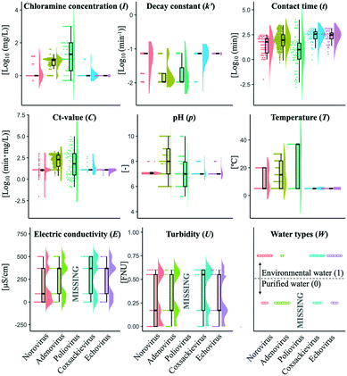
The summary of the available variables in this study is shown in Fig. 1. Initial chloramine concentration (I) included several higher values (more than 10 mg L⁻¹) in 46% of the datasets of poliovirus disinfection while almost all I values of norovirus, coxsackievirus and echovirus studies were around 1 mg L⁻¹. The logarithmic Ct-values (C) of the coxsackievirus and echovirus were less diverse. The values of pH (p) and temperature (T) of the adenovirus studies varied, whereas those of T in the other virus studies were distributed around 5 °C. Only identical values of I, k′ and T in the echovirus datasets and those of T in the coxsackievirus datasets were found. Disinfection tests of poliovirus did not describe the information about electric conductivity (E), turbidity (U) and water types (W) (0: purified, 1: environmental water) (Table S1,†Fig. 1). Several datasets did not include information about E and U, so the mean imputation was applied to compensate for such missing values when the dataset was obtained in a disinfection experiment using environmental water. When an experiment was conducted in purified water, missing values of E and U were replaced with one and zero, respectively. We prepared three models, in which all missing variables were imputed by mean, zero or maximum values, and a model without imputation to validate the effect of imputations on the prediction performance. The imputation did not affect the prediction performance (Fig. S3†). Raw data analysed in this study are available in the ESI† file.

Fig. 1 Available water quality parameters. Nine water quality parameters were plotted for each virus as swarm (left), box (center) and violin (right) plots. Box plots indicates median, 25 percentile, 75 percentile, minimum and maximum values.

Prediction of LRVs by regularized regression analyses

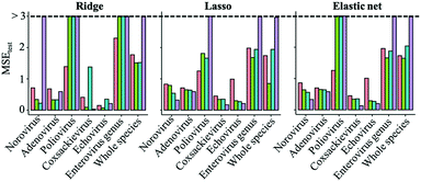
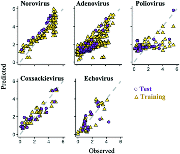
Regularized regression analysis includes ridge, lasso and elastic net regressions. Ridge regression uses all variables with shrinking coefficient values. On the other hand, lasso and elastic net regression analyses, called sparse modeling, are able to extract essential variables and eliminate non-essential ones from the prediction model. The sparse modeling method has been used in various research fields.^28,29,45,46

The prediction performances of the three regularized regression analyses for the test datasets (trial 1) were evaluated using MSE values (Fig. 2). Compared to virus specific models, MSE values of genus enterovirus (poliovirus, coxsackievirus and echovirus) and whole virus species models were higher, so the predictive inactivation models are needed to be established for each virus species. The addition of interaction-cubic terms decreased the prediction performances in some models based on the ridge regression probably because there remained too many variables in the ridge regression with interaction-cubic terms. On the other hand, MSE values were lower in all the predictive inactivation models based on sparse estimation with higher terms except for poliovirus. It seemed that the model using only linear terms was appropriate for predicting poliovirus LRVs. For other viruses, sparse-based models with interaction-cubic terms or ridge-based models with interaction terms could give higher prediction performance. However, training and test datasets were divided from the same articles, and thus the test datasets were likely to correlate to the training datasets in trial 1, and there was a possibility that prediction performances were over-estimated.

Fig. 2 Mean squared errors (MSEs) calculated by ridge, lasso and elastic net regression analyses for the test datasets (trial 1). MSEs of models with linear (red), interaction (green), interaction-quadratic (blue) and interaction-cubic (purple) terms are arranged from left to right for each virus species.

Determination of the best regularized regression model

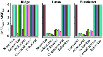
To identify which models were capable of avoiding an exaggeration of prediction performance and were appropriate for LRV predictions, we used datasets from an article which has the smallest dataset size as test datasets and then compared the MSEs between the training and test datasets (trial 2) (Fig. 3). If the MSE difference is smaller, the model is unlikely to overfit to the training datasets and can be suitable to predict new datasets. Differences of the MSE between the test and training data were larger in models based on the ridge regression analysis. Although the prediction performances were better than those of sparse modeling methods when using test data related to training datasets (trial 1, Fig. 2), ridge-based models have a risk of overfitting to training datasets (Fig. 3) and failing to predict new datasets. Lasso- and elastic net-based models made the MSE differences between the test and training datasets smaller than ridge-based ones.

Fig. 3 Comparison of mean squared errors (MSEs) calculated by ridge, lasso and elastic net regression analyses between the training and test datasets (trial 2). Absolute values of the MSEs of the models with linear (red), interaction (green), interaction-quadratic (blue) and interaction-cubic (purple) terms are arranged from left to right for each virus species.

Norovirus models based on lasso and elastic net regression greatly decreased the MSE differences by adding quadratic or cubic terms (Fig. 3). MSE differences of adenovirus and poliovirus models were slightly affected by introducing higher terms. The additions of higher terms to coxsackievirus and echovirus models made the MSE differences larger probably because of the smaller size of datasets and variables. Sparse modeling with linear terms was suitable for predicting coxsackievirus LRVs. Because the datasets of the echovirus were obtained from only two articles, overfitting to the training datasets (from only one article) could be inevitable in the current datasets, but the MSE_test values in sparse-based models with linear terms were ten times as small as those with higher terms (Table S4†).

The selection of variables is vital to model construction,⁴⁷ and the addition of extra variables to a model can cause multicollinearity, in which the accuracy of prediction is superficially improved.⁴⁸ Regularized regression analyses solve the issues caused by multicollinearity, which is supported by the variance inflation factor (Table S3†), and in this study, we demonstrated that a sparse estimation made it possible to avoid overfitting to the training datasets. When MSE values are similar between models based on lasso and elastic net or the models with lower and higher terms, we judge that the lasso based-model with small number of variables^28,29 and lower terms is appropriate for the predictive model (trial 1). Also, models that have the smaller absolute value of MSEs between test and training datasets are preferred, and are possible to avoid overfitting (trial 2). Together, the best fit models are the lasso-based model with interaction-quadratic terms (norovirus), that with only interaction terms (adenovirus) and the elastic net based-model with linear terms (poliovirus, coxsackievirus and echovirus).

Features of the best regularized regression model

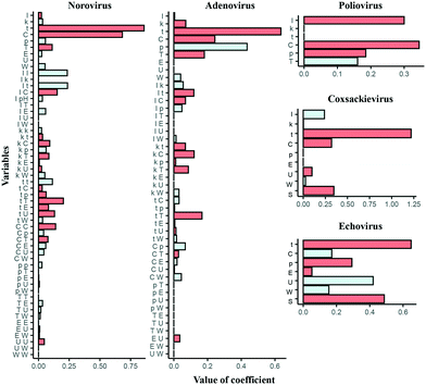
All the best regularized regression models include higher coefficient of t, except for the poliovirus model where the coefficient of I is higher (Fig. 4). The coefficient of C is also higher among all the models but the echovirus model has a negative coefficient of C. The negative coefficient C means that the coefficient C approaches threshold values as t increases because of the negative exponential function (eqn (2)). Also, both I and k′ take single values in all the echovirus datasets, which results in less diversity of the value of C. Other water quality parameters such as p and T are also regarded as important while in norovirus models, some coefficients of interaction terms are higher than those of linear terms such as p, T, and U. Interaction terms are possibly substituted with essential variables that are absent in some reports. In contrast to statistical models, physical, chemical and microbiological interpretations of the selected variables are usually difficult in machine learning algorithms because the feature engineering (e.g., the addition of polynomial terms) aims to just make a model more predictable. However, if more information about water quality and operational parameters with LRV data are available in the future, we don't need to add higher terms and can update the predictive inactivation models, which is more intuitive.

Fig. 4 Coefficients of the best models identified by the regularized regression analyses (red: positive, pale blue: negative). Letters indicate the type of variables (I: initial concentration of chloramine, t: contact time, k: decay constant of chloramine, C: Ct-value, p: pH, T: temperature, E: electric conductivity, U: turbidity, W*: water types (purified or environmental water), S*: type of strain, *: dummy variables).

Does the hierarchical Bayesian approach improve models?

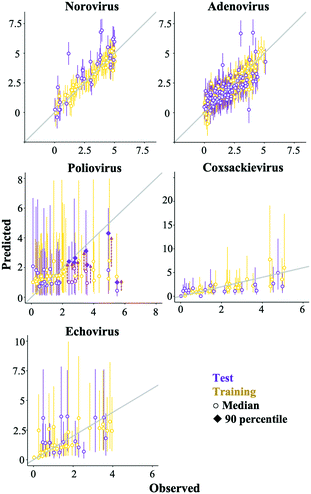
Some prediction values of the best regularized regression models were largely deviated from the observed test data, especially in the poliovirus model (Fig. 5). The prediction results of the coxsackievirus and echovirus models implied that the strain type was an important factor for predicting enterovirus LRVs (Fig. 4), so the hierarchical Bayesian approach,²¹ which took more than three types of strain into account, was likely to improve the LRV prediction for the poliovirus. In addition, it is possible to take into account the effect of experimental conditions, which are not recorded in the articles on the LRV prediction by the approach.²¹ The probability distributions of the LRV of each virus species were determined based on AIC (Table S2†). The variables selected by the best fit models based on the regularized regression analyses (Table 4) were applied here. The hierarchical Bayesian approach improved the prediction performance only for the training datasets of norovirus, adenovirus and poliovirus (Table 3). The 95% confidence intervals estimated by the models of each enterovirus are broader (Fig. 6) probably due to the small number of datasets and/or the strong strain-dependent sensitivity to chloramine (Table 2). No improvement on the prediction for the test datasets was found, but in the poliovirus model, the prediction performance for higher LRVs can be improved by the Bayesian approach. When we focus on the 90 percentiles of more than 2 LRVs of the poliovirus, the prediction values become close to the observed ones (Fig. 6). The hierarchical Bayesian approach using fat-tailed distributions such as gamma (poliovirus and echovirus) and Weibull distributions (coxsackievirus) can be thus effective to correct the prediction for higher LRVs (Table S2†).

Fig. 5 Comparison of the observed data (yellow triangle) with the predicted values (purple circle) by the best regularized regression models. Grey dashed lines indicate that a predicted value completely matches an observed point.

Table 3 Mean squared errors of the best regularized regression and hierarchical Bayesian models

	The best regularized regression model		Hierarchical Bayesian model
	Train	Test	Train	Test
Norovirus	0.41	0.54	0.16	1.68
Adenovirus	0.62	0.65	0.28	0.84
Poliovirus	1.64	1.26	1.56	3.17
Coxsackievirus	0.30	0.45	1.30	1.81
Echovirus	0.44	0.92	0.62	1.87

---

Fig. 6 Comparison of the observed data (pale yellow) with the predicted values (purple) by the hierarchical Bayesian models with variables used in the best regularized regression models. Edges of the bars imply the 2.5 (lower) and 95 percentiles (upper), respectively. In the poliovirus model, the 90 percentiles (filled diamond) are also displayed.

Challenges for developing prediction models

The prediction performance of our models based on lasso or elastic net regression can be improved because, at present, some essential variables are possibly absent in the literature, and the diversity of the variable values is small (Fig. 1). In poliovirus disinfection, both the regularized regression and its expanded models by the hierarchical Bayesian were not able to precisely predict higher LRVs (Table 3 and Fig. 5), in which the number of model variables was the smallest (six variables) since information about electric conductivity, turbidity and type of water was missing (Fig. 1). Some predicted values of the echovirus model were also deviated from the observed ones in contrast to other virus species, and the model has only seven linear terms (Fig. 1 and 5). The echovirus model was established using approximately 50 datasets. The number of datasets of the coxsackievirus was also about 50, but the number of variables was 9, and both the test and training data were well predicted (Fig. 4 and 5). It is plausible that the number of and/or variety of water quality and operational parameters are required to improve the prediction performance.

We need to continue to collect new information about chloramine disinfection from future studies or suggest the creation of an internet site that allows everyone to access the disinfection data with water quality information from WWTPs as well as the Global Water Pathogen Project (GWPP; https://www.waterpathogens.org/). We also did not consider the effect of outliers on the LRV prediction. Approximately 46% of poliovirus LRVs are derived from disinfection tests that use more than 10 mg L⁻¹ of chloramine (Fig. 3a), which is an unrealistic condition (about 2.7 mg L⁻¹) at almost all WWTPs.⁴⁹ Prediction performance would surely be improved by processing outliers in combination with the “domain knowledge”, which is the specialized scientific knowledge selecting practical and appropriate datasets to predict LRVs of enteric viruses in wastewater.⁵⁰

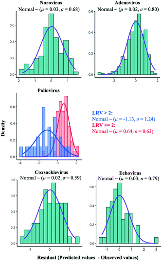
An alternative approach to improve the current best models is to add an error distribution. We focused on the distances of the predicted values by the models in trial 1 from the observed ones (Fig. 5) and plotted the distances as histograms, called error distributions, for each virus species in Fig. 7. Given the new datasets about water quality and operational information, the models established here can correct predicted values and provide confidence intervals by adding error distributions to the predicted values (Fig. 7). Note that we have to appropriately use the bimodal error distributions of the poliovirus according to the estimated LRV (if the predicted LRV is more than two, the broader error distribution needs to be applied (Fig. 7)) since the poliovirus model has less prediction performance for higher LRVs compared to lower LRVs (Fig. 5). The error distributions should be updated along with the models when new datasets for LRVs are available.

Fig. 7 Probability distributions of the distances between the observed and predicted values by the best regularized regression based-models. Lines are drawn by the best fitted probability density function. Only the poliovirus histogram is bimodal, so two probability distributions are depicted (observed values are two or less (red) or over two (blue)).

Application of the predictive inactivation model to determine the CL at WWTPs

Currently, we don't have a correct and common approach to determine the CL at WWTPs. There are some descriptions about the current CLs,⁵¹ but it is unclear how to determine CLs in many WWTPs. The Australian government provides a guideline employing HACCP for a water treatment plant, where CLs for disinfection include not only viruses but also bacteria and protozoa.⁵² Because the model for whole virus species constructed here has the worse prediction performance than models developed for individual species (Fig. 2), the CL for virus disinfection should be determined by taking the inactivation profiles of each virus species into account.

In this study, we provided the framework for the construction of predictive virus inactivation models and found that sparse modeling methods that avoided overfitting to training datasets were appropriate for the prediction of virus LRVs (Table 4). When datasets for other viruses and even other microbes are available, the modeling framework based on the sparse estimation can be also useful to predict their LRVs. Application of predictive inactivation models helps WWTP operators to recognize the difference of the present LRV from the target LRV^14,15 by inputting operational and water quality parameters. Then, several operational parameters (e.g., disinfectant concentration, contact time and Ct-value) change to achieve the target LRV.

Table 4 The current best models for predicting virus LRVs

	Algorithm	Polynomial terms
Norovirus	Lasso	Quadratic
Adenovirus	Lasso	Interaction
Poliovirus	Elastic net (LRV <2)	Linear
	Hierarchical Bayesian (LRV> = 2)
Coxsackievirus	Elastic net	Linear
Echovirus	Elastic net	Linear

---

Conclusions

LRVs have been estimated by simple mathematical models (Chick–Watson, Hom and efficiency factor Hom (EFH) models).^53,54 These models do not include the effects of water quality, which impacts virus LRVs.^55,56 In this study, we established predictive inactivation models in chloramine disinfection by regularized regression analyses, in which the water quality parameters were used as explanatory variables. Our established models estimated LRVs by inputting several water quality and operational parameters, and were able to avoid over- and/or under-estimation of the LRV by combining hierarchical Bayesian or using error distributions, which can be applied for each WWTP treating different water qualities.

The CL can be determined by employing our predictive models, which achieve virus concentration corresponding to the suggested reference value of tolerable infectious risks and disease burden (DALY loss per person per year).^57,58 Schmidt et al. have recently demonstrated that an effective LRV, weighted with a flow rate, is more suitable for the average performance of water treatment and risk calculation in QMRA. The LRV predicted by the best models suggested here can be applied to estimate the effective LRV, which avoids an underestimation of the risk of infection.⁵⁹ Our models based on the sparse modeling enable WWTP operators and risk assessors to determine proper CLs at WWTPs to reduce enteric viruses in wastewater, although we need to continue the collection of LRV data with water quality information and revise the models periodically in order to construct more robust versions.

Conflicts of interest

There are no conflicts to declare.

Acknowledgements

This study was supported by the Gesuido Academic Incubation to Advanced Project, Japan Ministry of Land, Infrastructure, Transport and Tourism and “The Sanitation Value Chain: Designing Sanitation Systems as Eco-Community Value System” Project, Research Institute for Humanity and Nature (RIHN, Project No. 14200107).

References

1. M. N. Subahir, M. S. Jeffree, M. Hassan, S. M. G. Mohamad, S. Y. Fong and K. Ahmed, Norovirus outbreak among students of a boarding school in Kluang, Johor, Malaysia, J. Infect. Dev. Countries, 2019, 13(4), 274–277.
2. S. A. Hoque, M. Kobayashi, S. Takanashi, K. S. Anwar, T. Watanabe, P. Khamrin, S. Okitsu, S. Hayakawa and H. Ushijima, Role of rotavirus vaccination on an emerging G8P[8] rotavirus strain causing an outbreak in central Japan, Vaccine, 2018, 36, 43–49.
3. C. Croker, S. Hathaway, S. Marutani, M. Hernandez, C. Cadavid and S. Rajagopalan, Outbreak of hepatitis A virus infection among adult patients of a mental hospital – Los Angels county, 2017, Infect. Control Hosp. Epidemiol., 2018, 39(7), 881–882.
4. M. Bauri, A. L. Wilkinson, B. Ropa, K. Feldon, C. J. Snider, A. Anand, G. Tallis, L. Boualam, V. Grabovac, T. Avagyan, S. M. Reze, D. Mekonnen, Z. Zhang, B. R. Thorley, H. Shimizu, L. N. G. Apostol and Y. Takashima, Circulating vaccine-derived poliovirus type 1 and outbreak response – Papua New Guinea, 2018, Morb. Mortal. Wkly. Rep., 2019, 69(5), 119–120.
5. J. Li, X. Lu, Y. Sun, C. Lin, F. Li, Y. Yang, Z. Liang, L. Jia, L. Chen, B. Jiang and Q. Wang, A swimming pool-associated outbreak of pharyngoconjunctival fever caused by human adenovirus type 4 in Beijing, China, Int. J. Infect. Dis., 2018, 75, 89–91.
6. H. Katayama, E. Haramoto, K. Oguma, H. Yamashita, A. Tajima, H. Nakajima and S. Ohgaki, One-year monthly quantitative survey of noroviruses, enteroviruses, and adenoviruses in wastewater collected from six plants in Japan, Water Res., 2008, 42, 1441–1448.
7. M. A. Adefisoye, U. U. Nwodo, E. Green and A. I. Okoh, Quantitative PCR detection and characterization of human adenovirus, rotavirus and hepatitis A virus in discharged effluents of two wastewater treatment facilities in the Eastern Cape, South Africa, Food Environ. Virol., 2016, 8, 262–274.
8. A. D. Schlindwein, C. Rigotto, C. M. O. Simoes and C. R. M. Baradi, Detection of enteric viruses in sewage sludge and treated wastewater effluent, Water Sci. Technol., 2010, 61(2), 537–544.
9. WHO, Guidelines for the use of wastewater, excreta and greywater in agriculture and aquaculture, World Health Organization, Geneva, 3rd edn, 2006.
10. WHO, Sanitation safety planning: Manual for safe use and disposal of wastewater, greywater and excreta, World Health Organization, Geneva, 2015.
11. Codex Alimentarius Commision, Basic texts on food hygiene, Codex Alimentarius Commission, Rome, 4th edn, 2009.
12. M. Y. Lim, J.-M. Kim and G. P. Ko, Disinfection kinetics of murine norovirus using chlorine and chlorine dioxide, Water Res., 2010, 44(10), 3243–3251.
13. N. Dunkin, S. C. Weng, C. G. Coulter, J. G. Jacangelo and K. J. Schwab, Impacts of virus processing on human norovirus GI and GII persistence during disinfection of municipal secondary wastewater effluent, Water Res., 2018, 134, 1–12.
14. T. Ito, M. Kitajima, T. Kato, S. Ishii, T. Segawa, S. Okabe and D. Sano, Target virus log10 reduction values determined for two reclaimed wastewater irrigation scenarios in Japan based on tolerable annual disease burden, Water Res., 2017, 125(15), 438–448.
15. D. Sano, M. Amarasiri, A. Hata, T. Watanabe and H. Katayama, Risk management pf viral infectious diseases in wastewater reclamation and reuse: Review, Environ. Int., 2016, 91, 220–229.
16. D. Li, A. Z. Gu, S. Zeng, W. Yang, M. He and H. Shi, Evaluation of the infectivity, gene and antigenicity persistence of rotaviruses by free chlorine disinfection, J. Environ. Sci., 2011, 23(10), 1691–1698.
17. N. Dunkin, S. Weng, J. K. Schwab, J. McQuarrie, K. Bell and J. G. Jacangelo, Comparative inactivation of murine norovirus and MS2 bacteriophage by peracetic acid and monochloramine in municipal secondary wastewater effluent, Environ. Sci. Technol., 2017, 51, 2972–2981.
18. Y. Park, M. Kim, Y. Pachepsky, S.-H. Choi, J.-G. Cho, J. Jeon and K. H. Cho, Development of a nowcasting system using machine learning approaches to predict fecal contamination levels as recreational Beaches in Korea, J. Environ. Qual., 2018, 47, 1094–1102.
19. H. Lu and X. Ma, Hybrid decision tree-based machine learning models for short-term water quality prediction, Chemosphere, 2020, 249, 126169.
20. M. J. S. Safari, S. R. Arashloo and A. D. Mehr, Rainfall-runoff modeling through regression in the reproducing kernel Hilbert space algorithm, J. Hydrol., 2020, 587, 125014.
21. S. Kadoya, O. Nishimura, H. Kato and D. Sano, Predictive water virology: Hierarchical Bayesian modeling for estimating virus inactivation curve, Water, 2019, 11(10), 2187.
22. D. G. Sharp and L. Leong, Inactivation of poliovirus-I (Brunhilde) single poliovirus particles by chlorine in water, Appl. Environ. Microbiol., 1980, 40, 381–385.
23. R. Floyd, D. G. Sharp and J. D. Johnson, Inactivation by chlorine of single poliovirus particles in water, Environ. Sci. Technol., 1979, 13, 438–442.
24. M. Amarasiri, S. Hashiba, T. Miura, T. Nakagomi, O. Nakagomi, S. Ishii, S. Okabe and D. Sano, Bacterial histo-blood group antigens contributing to genotype-dependent removal of human noroviruses with a microfiltration membrane, Water Res., 2016, 95, 389–391.
25. D. Moher, A. Libeerati, J. Tetzlaff and D. G. Altman, Preferred reporting items for systematic reviews and meta-analysis: the PRISMA statement, PLoS Med., 2009, 6, e1000097.
26. C. A. Shneider, W. S. Rasband and K. W. Eliceiri, NIH image to Image J: 25 years of image analysis, Nat. Methods, 2012, 9(7), 671–675.
27. A. E. Hoerl and R. W. Kennard, Ridge regression: Biased estimation for nonorthogonal problems, Technometrics, 1970, 12(1), 55–67.
28. R. Tibshirani, Regression shrinkage and selection via the lasso, J. R. Stat. Soc. Series. B., 1996, 36, 117–147.
29. H. Zou and T. Hastie, Regularization and variable selection via the elastic net, J. R. Stat. Soc. Series. B., 2006, 67, 301–320.
30. M. L. Delignette-Muller and C. Dutang, fitdistrplus: An R package for fitting distributions, J. Stat. Softw., 2015, 64(4), 1–34.
31. K. Sirikanchana, J. L. Shisler and B. J. Marinas, Inactivation kinetics of adenovirus serotype 2 with monochloramine, Water Res., 2008, 42, 1467–1474.
32. K. Sirikanchana, J. L. Shisler and B. J. Marinas, Effect of exposure to UV-C irradiation and monochloramine on adenovirus serotype 2 early protein expression and DNA replication, Appl. Environ. Microbiol., 2008, 74(12), 1467–1474.
33. E. Lund, Inactivation of poliomyelitis virus by chlorination at different oxidation potentials, Arch. Virol., 1961, 11(3), 330–342.
34. E. Lund, Effect of pH on the oxidative inactivation of poliovirus, Arch. Virol., 1962, 12(5), 632–647.
35. A. M. Gall, J. L. Shisler and B. J. Marinas, Inactivation kinetics and replication cycle inhibition of adenovirus by monochloramine, Environ. Sci. Technol. Lett., 2016, 3, 185–189.
36. C. S. Baxrer, R. Hoffman, M. R. Templeton, M. Brown and R. C. Andrews, Inactivation of adenovirus types 2, 5, and 41 in drinking water by UV light, free chlorine, and monochloramine, J. Environ. Eng., 2007, 133(1), 95–103.
37. T. L. Cromeans, A. M. Kahler and V. R. Hill, Inactivation of adenoviruses, enteroviruses, and murine norovirus in water by free chlorine and monochloramine, Appl. Environ. Microbiol., 2009, 76(4), 1028–1033.
38. M. D. Sobsey, T. Fujii and P. A. Shields, Inactivation of hepatitis A virus and model viruses in water by free chlorine and monochloramine, Water Sci. Technol., 1988, 20(11/12), 385–391.
39. N. M. M. Gowda, N. M. Trieff and G. J. Stanton, Inactivation of poliovirus by chloramine-T, Appl. Environ. Microbiol., 1981, 42(3), 469–476.
40. N. M. M. Gowda, N. M. Trieff and G. J. Stanton, Kinetics of inactivation of adenovirus in water by chloramine-T, Water Res., 1984, 20(7), 817–823.
41. G.-A. Shin and M. D. Sobsey, Reduction of norwalk virus, poliovirus 1 and coliphage MS2 by monochloramine disinfection of water, Water Sci. Technol., 1988, 38(12), 151–154.
42. A. M. Kahler, T. L. Cromeans, J. M. Roberts and V. R. Hill, Source water quality effects on monochloramine inactivation of adenovirus, coxsackievirus, echovirus and murine norovirus, Water Res., 2011, 45, 1745–1751.
43. Z. Cui and G. Gong, The effect of machine learning regression algorithms and sample size on individualized behavioral prediction with functional connectivity features, NeuroImage, 2018, 178, 622–637.
44. J. Leonard, J. Flournoy, C. P. L-de. los Angeles and K. Whitaker, How much motions is too much motion? Determining motion thresholds by sample size for reproducibility in developmental resting-state MRI, Res. Ideas Outcomes, 2017, 3, e12569.
45. T. Kawashima, M. Kino and K. Akiyama, Black hole spin signature in the black hole shadow of M87 in the flaring state, Astrophys. J., 2019, 878(1), 27–36.
46. M. Lustig, D. Donoho and J. M. Pauly, Sparse MRI: The application of compressed sensing for rapid MR imaging, Magn. Reson. Med., 2007, 58, 1182–1195.
47. S. Abdul-Wahab, C. S. Bakheit and S. M. Al-Alawi, Principal component and multiple regression analysis in modeling of ground-level ozone and factors affecting its concentrations, Environ. Modell. Softw., 2005, 20, 1263–1271.
48. J. Jaccard, C. K. Wan and R. Turrisi, The detection and interpretation of interaction effects between continuous variables in multiple regression, Multivariate Behav. Res., 1990, 25(4), 467–478.
49. C. J. Seidel, M. J. Mcguire, R. S. Summers and S. Via, Have utilities switched to chloramines?, J. - Am. Water Works Assoc., 2005, 97(10), 87–97.
50. T. Kato, A. Kobayashi, W. Oishi, S. Kadoya, S. Okabe, N. Ohta, M. Amarasiri and D. Sano, Sign-constrained linear regression for prediction of microbe concentration based on water quality datasets, J. Water Health, 2019, 17(3), 404–415.
51. WateReuse Research Foundation, Utilization of hazard analysis and critical control points approach for evaluating integrity of treatment barriers for reuse, WateReuse Research Foundation, USA, 2014.
52. NHMRC and NRMMC, Australian drinking water guidelines paper 6 National water quality management strategy, Natural Health and Medical Research Council, National Resource Management Ministerial Council, Canberra, Australia, 2011.
53. L. W. Hom, Kinetics of chlorine disinfection in an ecosystem, Journal of the Sanitary Engineering Division, 1972, 98(1), 183–193.
54. C. N. Hass and J. Joffe, Disinfection under dynamic conditions: Modification of Hom's model for decay, Environ. Sci. Technol., 1994, 28, 1367–1369.
55. S. Wati, B. S. Robinson, J. Mieog, J. Blackbeard and A. R. Keegan, Chlorine inactivation of coxsackievirus B5 in recycled water destined for non-portable reuse, J. Water Health, 2019, 17(1), 124–136.
56. T. Miura, A. Gima and M. Akiba, Detection of norovirus and rotavirus presents in suspended and dissolved forms in drinking water sources, Food Environ. Virol., 2019, 11, 9–19.
57. U. S. Environmental Protection Agency, Risk assessment guidance for superfund (RAGS) Volume III, part A, USEPA, Washington, DC, 1990.
58. WHO, WHO methods and data sources for global burden of disease estimates 2000–2015, World Health Organization, Geneva, Switzerland, 2017.
59. P. J. Schmidt, W. B. Anderson and M. B. Emelko, Describing water treatment process performance: Why average log reduction can be a misleading statistic, Water Res., 2020, 176, 115702.

---

Footnote

† Electronic supplementary information (ESI) available. See DOI: 10.1039/d0ew00539h

---