DOI:
10.1039/C9SM01462D
(Paper)
Soft Matter, 2019,
15, 9120-9132
A simulation study of aggregation mediated by production of cohesive molecules†
Received
18th July 2019
, Accepted 12th September 2019
First published on 23rd September 2019
Abstract
Mechanical interactions between biological cells can be mediated by secreted products. Here, we investigate how such a scenario could affect the cells' collective behaviour. We show that if the concentration field of secreted products around a cell can be considered to be in steady state, this scenario can be mapped onto an effective attractive interaction that depends on the local cell density. Using a field-theory approach, this density-dependent attraction gives rise to a cubic term in the Landau–Ginzburg free energy density. In continuum field simulations this can lead to “nucleation-like” appearance of homogeneous clusters in the spinodal phase separation regime. Implementing the density-dependent cohesive attraction in Brownian dynamics simulations of a particle-based model gives rise to similar “spinodal nucleation” phase separation behaviour.
Introduction
Living cells can secrete a plethora of molecules that allow them to interact with nearby cells. Secreted molecules can act as signals affecting gene expression (as in quorum sensing1,2) or motility (as in chemotaxis3). They can also, directly or indirectly, affect mechanical interactions between cells. For example, secreted proteins and polysaccharides influence cell–cell cohesion and cell clustering4 in processes ranging from morphogenesis in human tissue5 to fruiting body formation in spore-forming bacteria.6 In the assembly of bacterial biofilms on surfaces, polymer production plays an important role in mediating cohesive interactions.7,8 Many bacteria also form aggregates in liquid suspension,9–11 with significant industrial12,13 and clinical14–16 implications. For the bacterium Pseudomonas aeruginosa, the secretion of DNA9 and polysaccharides17 have been found to be important for aggregate formation.
A system of living cells that actively secrete a cohesion-influencing chemical agent (be it a polymer or signal molecule) is clearly out of equilibrium. Yet, even for out-of-equilibrium living organisms, useful mappings can often be made to key concepts in soft matter and statistical physics.18–27 Importantly, the case we investigate here, in which the cohesion-inducing agent is actively produced, is quite different to “passive” scenarios in which a cohesion-inducing agent (e.g., a polymer) is added to a system of cells or colloidal particles.24,28–32 In the latter cases, the polymer concentration is conserved; in the case that we consider here, the cohesive agent is constantly produced and degraded, and hence is not conserved.
In this paper, we investigate the collective behaviour of a system of aggregating particles secreting a cohesion-inducing agent. We follow previous studies in active matter physics,19,21–24,26 by considering aggregation as a phase separation process, albeit here our focus is on cell–cell cohesion and not activity arising from cellular motility. First, we formulate a mathematical model that shows that a system of particles producing a cohesion-inducing agent under steady-state conditions can be coarse-grained via an effective attractive interaction that depends on the local particle density. Taking a field-theory approach, this density dependence gives rise to a cubic term in the Landau–Ginzburg free energy that alters the thermodynamic landscape in comparison to that of a standard, density-independent model. Computer simulations of the Cahn–Hilliard equation also show different dynamics during early-stage phase separation for the density-dependent versus density-independent systems. Specifically, for the density-dependent system we observe “nucleation-like” appearance of homogeneous particle clusters in the spinodal decomposition regime. Similar emergent behaviour arises when the density-dependent cohesion is implemented in particle-based Brownian Dynamics simulations.
Mathematical model
To motivate the use of an effective attractive interaction to model systems of particles secreting a cohesion-inducing agent, we first study a simple diffusion problem. We consider the secretion of a cohesion-inducing chemical agent by a spherical source particle of radius δ such as that depicted in Fig. 1. We assume that the cohesion-inducing agent has diffusion constant D and degrades at rate kd. The time evolution of its concentration field, c(r′,t), at radial distance r′ > δ from the centre of the source particle is given by the following reaction–diffusion equation in spherical coordinates| | 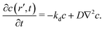 | (1) |
We solve this equation in the steady-state by requiring that its solution is finite at infinity, and that it satisfies the following boundary conditionwhere w is the flux of the cohesion-inducing agent through the surface of the particle. The solution is then given by| | 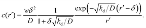 | (3) |
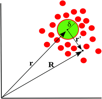 |
| | Fig. 1 Schematic illustration of cohesion-inducing agents (red disks) emanating from a source particle of radius δ (green). At the particle's surface, the flux of the cohesion-inducing agent is fixed according to eqn (2); this boundary condition imposes a diffusive flux of cohesive agent away from the source. | |
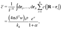
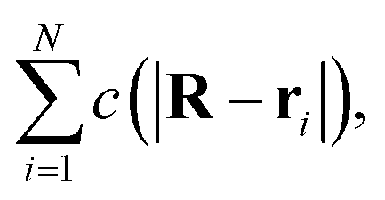
Consider now a collection of N such sources located at positions (r1, r2,…rN) in a volume V. The total concentration of the cohesion-inducing agent at a location R, sufficiently far away from the sources, can be approximated by
| |  | (4) |
where
c(
r′) is given by
eqn (3), and we neglected interactions between the sources, implying the dilute limit. The ensemble average over uniformly distributed positions of the sources finally gives
| |  | (5) |
where
ρ =
N/
V is the particle number density, and

. The ratio
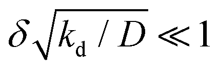
α compares the timescale for the cohesion-inducing agent to diffuse the size of the source particle, to the timescale of its degradation, and is assumed to be small in our steady-state regime.
33 With this is mind,
eqn (5) shows that the concentration of cohesion-inducing agents is a linear function of the particle number density
ρ,
33 and therefore we can expect cohesive interactions, which are mediated by these agents, to be a linear function of the local particle density (provided we are in the regime where the agent concentration can be considered to be in steady state). We also note that 4π
δ2w is the total amount of agent being secreted through the surface per unit time, and thus the prefactor in
eqn (5) is the ratio of the production rate to the degradation rate.
We now take a further step and assume that the cohesion-inducing agents can be treated in a coarse-grained manner, as an effective interaction between the particles. We suppose that the agents produce attractive forces between the particles, and that the degree of attraction is proportional to the local concentration of cohesive agents. Following our analysis above (in particular eqn (5)), this in turn implies that the degree of attraction depends on the local density of the particles themselves. Hence, our system can be modelled as a collection of particles interacting via a density-dependent attractive potential.
In soft matter physics, the concept of a density-dependent potential is not new: for example, density-dependent effective pair potentials arise when treating polymers as soft colloids, and when treating a two-component mixture as an effective one-component system, as in the Asakura-Oosawa model for polymer–colloid mixtures.34 It is well known that naive application of potentials that depend on the global particle density can lead to problems such as a lack of consistency between virial and compressibility routes to the equation of state.34 This problem appears to be alleviated in the case of interactions that depend on the local density, like those we consider here.34,35 Moreover, our model represents a non-equilibrium system, in which cohesive agents are continuously produced – for such a system we would not necessarily expect the rules of equilibrium thermodynamics to be obeyed.
We also note that in a real system of interacting biological cells, many other factors may be at play, including motility and cell growth and division. For the sake of simplicity, these factors are neglected here.
Free-energy formalism
We consider the aggregation of our agent-secreting particles as a phase separation process, in which a homogeneous suspension of particles come together to form condensed phase regions of higher density (aggregates). We address this via a Landau–Ginzburg-like free energy formalism.36 We first review this formalism for particles interacting via density-independent interactions, then discuss how it changes when the interaction depends on the local particle density.
Density-independent interactions.
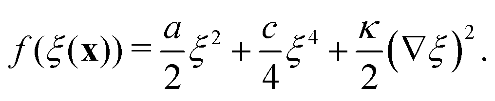
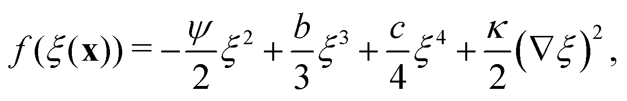
The canonical Landau–Ginzburg free energy density is usually expressed as an expansion of an order parameter field, ξ, about some critical value ξc. For the purposes of this work, ξ is a measure of the local particle density, defined such that ξc = 0. The free energy density can then be expressed as| | 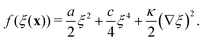 | (6) |
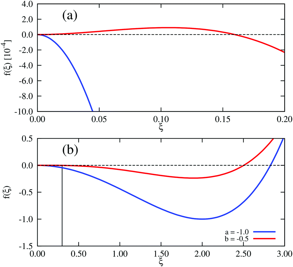
In Landau–Ginzburg theory, the phenomenological coefficients a and c often depend on the temperature. The coefficient a, which is a function of the deviation of the system temperature and the critical temperature (T − Tc), is the critical parameter that governs the transition between the disordered and ordered states. In our model, however, we will not consider this temperature dependence explicitly. Rather, in our Landau-like free energy density, eqn (6), we consider the ξ2 term as an effective two-body interaction in which the critical parameter a governs the transition between the disordered state in which entropic/repulsive interactions dominate, and the ordered state in which enthalpic/cohesive interactions dominate (Fig. 2(a)). Thus in our model a encapsulates a tradeoff between repulsive (ψ) and cohesive (υ) contributions, such that a = υ − ψ (analogous to the quadratic coefficient in the Bragg–Williams approximation for the Ising model37). We fix ψ arbitrarily to −0.05 so that the phase transition is governed by the value of υ, which represents the strength of the cohesive interactions. The quartic term in eqn (6) ensures that the equilibrium state has a bounded value of ξ, and thus must have a positive coefficient c > 0. The square gradient term imposes a free energy cost for any non-uniformity in ξ, and thus κ, which is related to the surface tension, must be positive. Note that we omit a positive cubic term in eqn (6), which is allowed by symmetry but would not affect our results, to facilitate numerical comparison to the density-dependent case described below.
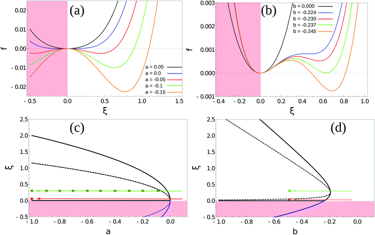 |
| | Fig. 2 Homogeneous part of the Landau–Ginzburg free energy density and the associated phase diagrams. (a) Free energy density, f(ξ), for various values of the critical parameter, a, in the density-independent system (eqn (6)). Note that the point ξ = 0 undergoes a continuous transition from a minimum to a maximum as a decreases through a = 0. Thus, this free energy density would produce a second-order phase transition in a system where the order parameter was not globally conserved. (b) Free energy density, f(ξ), for various values of the critical parameter, b, in the density-dependent system (eqn (11)). Note the emergence of a secondary minimum at ξ ≥ 0 as b decreases. Upon decreasing through b ∼ −0.237, where two equal free energy minima appear, the system would undergo a first-order phase transition if the order parameter was not globally conserved. (c and d) Phase diagrams generated by applying the common-tangent construction to the density-independent (c) and density-dependent (d) free energy profiles (see the ESI† for details). The black solid and dashed lines denote the binodal and spinodal coexistence lines respectively. Red arrows represent constant density quenches to the points (ξ = 0.07, a = −1.0, and ξ = 0.07, b = −0.5) within the coexistence regions of (c) and (d) respectively, as discussed in the text. Green arrows represent constant density quenches to the points (ξ = 0.3, a = −1.0, and ξ = 0.3, b = −0.5) within the coexistence regions of (c) and (d) respectively. | |
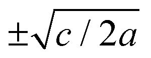
For positive values of the parameter a, the free energy density, eqn (6), has a single minimum at ξ = 0. In contrast, for negative values of a, eqn (6) has two minima at  . For the model represented by eqn (6) to be physically realistic, the condition of positive density, ξ ≥ 0, has to be imposed throughout, ruling out any equilibrium phase with ξ < 0. Fig. 2(a) shows the homogeneous part of the free energy density (eqn (6)); the region shaded red is inaccessible because it does not meet the condition ξ ≥ 0. The continuous transition from a state whereby ξ = 0 is the global minimum of the free energy density to a state where the global minimum is a positive finite value,
  , is a signature of the fact that this free energy density would produce a second-order phase transition in a system where the order parameter is not globally conserved.
Density-dependent interactions.
For particles that secrete a cohesion-inducing agent, we expect the cohesive interactions between particles to increase linearly with the local particle density (eqn (1)–(5)). If we consider the local particle density, ξ, in our Landau construction to be proportional to the density, ρ, in eqn (5), then we can express the attractive (enthalpic) parameter, υ, aswhere K is proportional to the ratio of the production and degradation rate (4πδ2w/kd) in eqn (5). More specifically, we choose to write| |  | (8) |
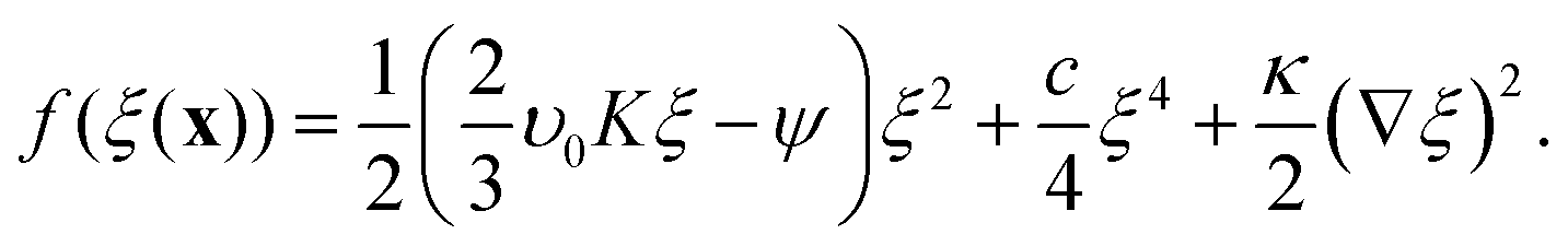
where we have introduced an arbitrary (constant) prefactor, υ0, to ensure the correct units of energy per unit volume (or area in 2D), and the factor of 2/3 ensures that the resulting free energy density will have a factor of 1/3 in the cubic term as standard. Substituting eqn (8) into the standard free-energy density expression, eqn (6), and using a = υ − ψ, gives| | 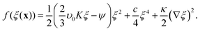 | (9) |
Expanding the first term in eqn (9) gives| |  | (10) |
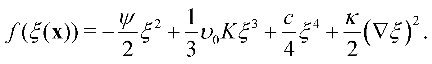
Defining a new parameter b = υ0K allows eqn (10) to be written as| |  | (11) |
and we fix ψ = −0.05 as before. We now have a different parameter, the coefficient b of the cubic term, that controls the phase transition. Fig. 2(b) shows the homogeneous part of the free energy density, eqn (11); the region shaded red is disallowed because ξ < 0. In this system, a free energy barrier emerges at low particle density ξ as the critical parameter b decreases, and gives rise to the region of metastability at low density that appears in the phase diagram of Fig. 2(d). This system therefore shows different physics to the density-independent one as the phase transition resulting from a decrease in b through its critical value, bc, is discontinuous; this would correspond to a first-order transition in systems with non-conserved order parameter (i.e., model A38) and is analogous to the isotropic–nematic transition in liquid crystals.39
In our model, particles are not created or removed (since we neglect cell growth or death), and therefore the density must be globally conserved. To minimise the free-energy density subject to this constraint, we apply the common-tangent construction to the homogeneous part of the free energy densities, eqn (6) and (11), to generate the density-independent and density-dependent phase diagrams shown in Fig. 2(c) and (d) respectively (see the ESI† for details). Importantly, the cubic term in the density-dependent system gives rise to a region of metastability (black dashed line) at small values of ξ that is absent in the density-independent system.
Field simulations
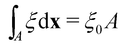
To determine the effects of the altered phase diagram on phase separation dynamics, we performed 2-dimensional numerical simulations of the density-independent and density-dependent models defined by eqn (6) and (11), to assess the effect of the free-energy barrier that emerges from the cubic term in the density-dependent case. Since ξ is a conserved order parameter (i.e.,  , where ξ0 is the overall system density and A is the total area), the phase-separation dynamics of the two systems can be modelled using the Cahn–Hilliard equation40
| | 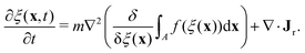 | (12) |
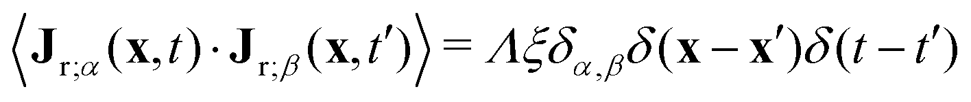
In eqn (12), m is the mobility, the term in brackets is the chemical potential, and Jr is a random flux which is spatially and temporally uncorrelated, i.e., 〈Jr(x,t)〉 = 0 and 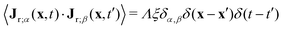 , with α,β = x, y. For simplicity, both m and the random noise strength Λ were kept constant, at m = 0.01 and Λ = 0.1.41Eqn (12) was solved on a 256 × 256 grid using standard finite difference simulations, with periodic boundary conditions.
Low-density quench.
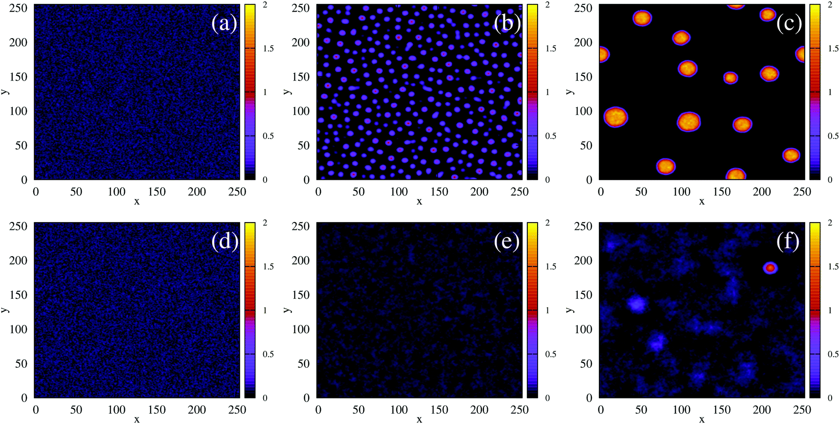
We first simulated the effect of quenching the system at low density (ξ = 0.07) from the homogeneous phase into the phase-separated region of the phase diagram. For the density-independent case, this corresponds to decreasing the parameter a as shown by the red arrow in Fig. 2(c) (a > 0 → a = −1.0). Since the system is quenched into the spinodal region of the phase diagram (Fig. 2(c)), we expect phase separation to occur via spinodal decomposition (a consequence of the negative curvature of the free energy function at ξ = 0.07 in Fig. 3(a)). Fig. 4(a)–(c) shows that this is indeed the case: the low density and high density phases separate spontaneously (see also Movie S1 in ESI†).
 |
| | Fig. 3 Free-energy governing low and high density quenches in the density-dependent and -independent systems. (a) Free energy densities of the density dependent system, b = −0.5, and its density-independent counterpart with a = −1.0. There is a small free energy barrier in the density-dependent system at small ξ (red curve). The black vertical line corresponds to the lower quench density, ξ = 0.07, which lies to the left of the barrier. Note that there is no barrier in the density-dependent case (blue curve). (b) The barrier is not evident when the free energy is plotted over larger ξ values. The black vertical line at ξ = 0.3 (higher quench density) lies to the right of the barrier in the density-dependent system. It provides a guide with which to visualise the curvature at the global density ξ0. The curvature (second derivative) of the free energy density at ξ0 is −0.1825 in the density-dependent case, and −0.9325 for the density-independent case: i.e., it is less negative in the density-dependent system. | |
 |
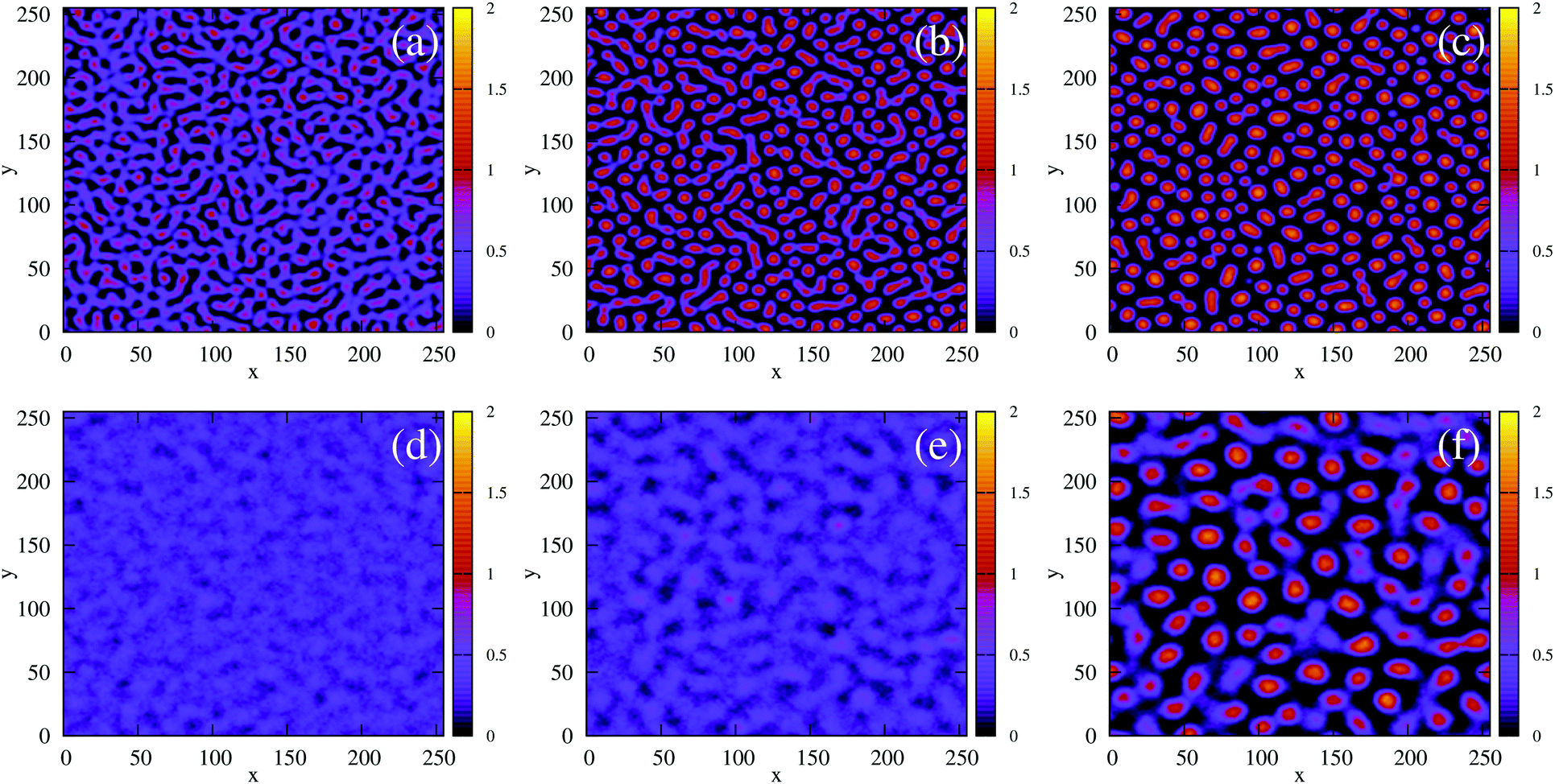
| | Fig. 4 The time evolution of the density-independent (a–c) and -dependent (d–f) systems following a quench highlights the effect of the free energy barrier at low density shown in Fig. 3. (a) Density-independent, ξ0 = 0.07, a = −1.0, at t = 0 SU. (b) Density-independent, ξ0 = 0.07, a = −1.0, at t = 250 SU. (c) Density-independent, ξ0 = 0.07, a = −1.0, at t = 47![[thin space (1/6-em)]](https://www.rsc.org/images/entities/char_2009.gif) 500 SU. (d) Density-independent, ξ0 = 0.07, b = −0.5, at t = 0 SU. (e) Density-independent, ξ0 = 0.07, b = −0.5, at t = 250 SU. (f) Density-independent, ξ0 = 0.07, b = −0.5, at t = 47500 SU. 500 SU. (d) Density-independent, ξ0 = 0.07, b = −0.5, at t = 0 SU. (e) Density-independent, ξ0 = 0.07, b = −0.5, at t = 250 SU. (f) Density-independent, ξ0 = 0.07, b = −0.5, at t = 47500 SU. | |
We also performed a similar quench for the density-dependent case. Here the parameter b was decreased as shown by the red arrow in Fig. 2(d) (b > 0 → b = −0.5), such that the resulting condensed phase density, ξcp ∼ 2, was similar to that of the density-independent system. In this case, the system is quenched into the low-density metastable region of the phase diagram (which does not exist for the density-independent case), and therefore we expect phase separation to occur via nucleation, requiring a large enough density fluctuation to overcome the free-energy barrier (red curve Fig. 3(a)). Indeed, the snapshots in Fig. 4(d)–(f) are consistent with nucleation: we observe the formation of a single aggregate that grows larger with time (see also Movie S2 in ESI†).
Higher-density quench.
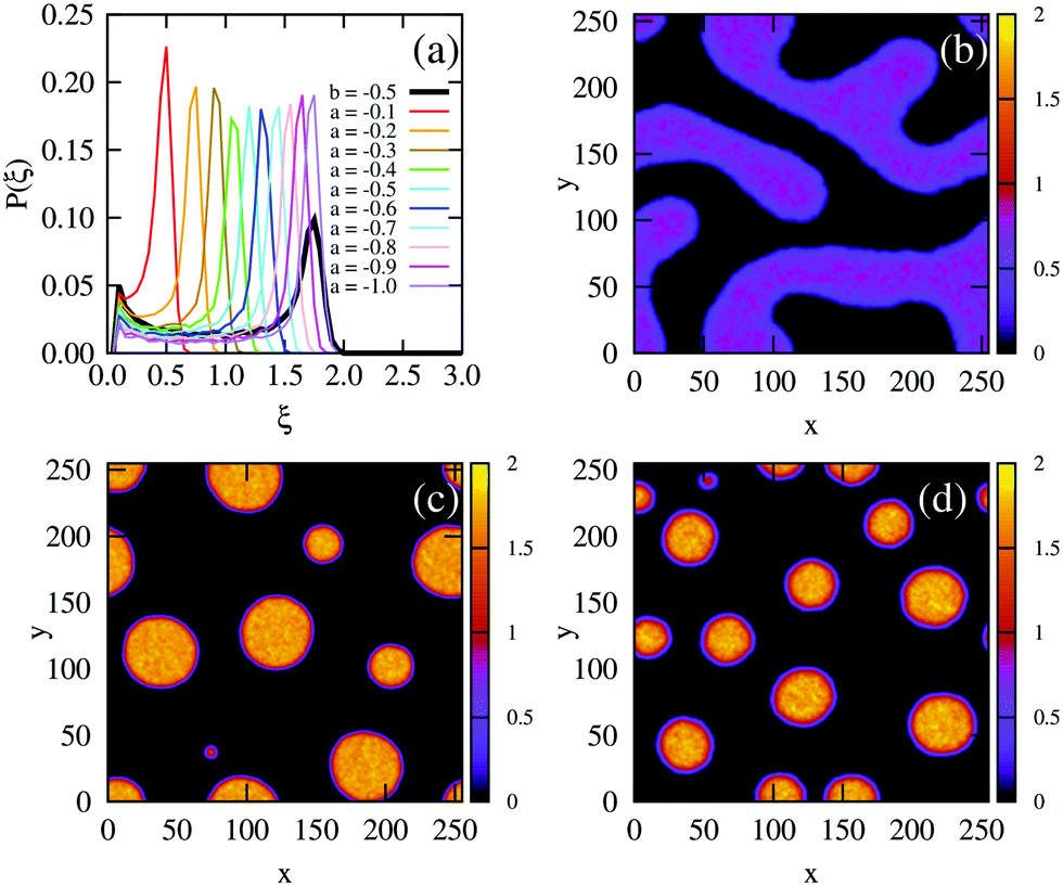
Next, we simulated a quench at the higher density of ξ = 0.3, which lies to the right of the free energy barrier in the density-dependent system (Fig. 3(b)). At this value of ξ, both the density-dependent and density-independent systems are quenched into the spinodal part of the phase diagram (green arrows in Fig. 2(c) and (d)). Let us first focus on the density-dependent case, for which the quench was performed from a homogeneous density at b > 0 to b = −0.5. Fig. 5(d) shows a snapshot of the system, taken at time t = 2.5 × 10⁵ simulation units (SU) following the quench. It is clear that phase separation does indeed proceed via spinodal decomposition (see also Movie S3 in ESI†), with many aggregates forming spontaneously. Fig. 5(a) (black line) plots the distribution of density values at this same time point; the distribution is clearly bimodal, with distinct peaks corresponding to the condensed and non-condensed phases.
 |
| | Fig. 5 Field simulations. (a) Probability distribution, P(ξ), of the order parameter ξ, at t = 2.5 × 10⁵ SU, for the density-dependent system (black curve), and the density-independent systems (coloured curves) at various values of the critical parameter a. The distributions shown were generated from one simulation run; distributions generated from repeated simulations showed no discernible differences (data not shown). (b) and (c) representative snapshots at t = 2.5 × 10⁵ SU of the density-independent system with a = −0.2 and a = −1.0 respectively, undergoing phase separation. (d) Representative snapshot at t = 2.5 × 10⁵ SU of the density-dependent system with b = −0.5, undergoing phase separation. It is reasonable to compare panels (c) and (d) since the density-independent system with a = −1.0 has a similar condensed phase density, ξcp ∼ 1.75, as the density-dependent system with b = −0.5. In all snapshots, the colour bar indicates the density. | |
We would like to know whether phase separation in the spinodal region differs intrinsically between the density-dependent and density-independent scenarios. To test this, we performed a series of quenches in the density-independent case, for ξ = 0.3, a > 0 initially, and a range of final a values (−0.1,−0.2, −0.3,…,−1.0; dark green points along the green line in Fig. 2(c)). The rationale for performing a range of simulations was that the density-dependent simulation effectively samples a range of υ values (since υ = 2/3υ0Kξ); thus many values of a should be sampled in the density-independent system in order to compare with the density-dependent case. Fig. 5(b) and (c) show snapshots of these simulations, for a = −0.2 and a = −1.0 respectively, taken at time t = 2.5 × 10⁵ SU following the quench. Clearly, the spinodal decomposition process is affected by the value of a: a more negative value of a produces a more rapid contraction of the early-stage elongated structures into the later-stage rounded clusters (see also Movie S4 (a = −0.2) and S5 (a = −1.0) in ESI†). The coloured lines in Fig. 5(a) show the distribution of density values at this same time point, for each of the density-independent simulations. These distributions are also bimodal, with a gas-phase peak at ξ ∼ 0.07 and a condensed-phase peak at a value ξcp that increases with decreasing a.
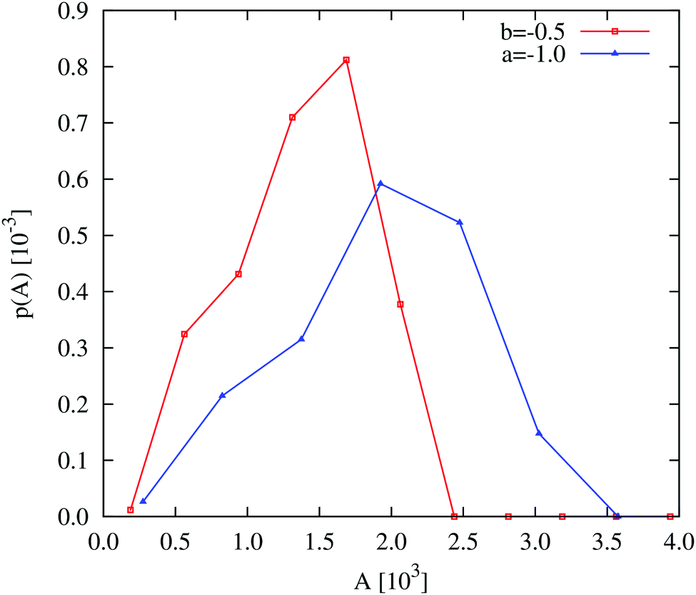
Comparing the density distributions in Fig. 5(a) between the density-dependent and density-independent cases (black vs. coloured lines), we see a notable difference: aggregate formation appears to be hindered in the density-dependent system. Specifically for the density-dependent case, the gas phase peak is larger, and the condensed phase peak is smaller. This points to a higher fraction of the gas phase coexisting with the condensed-phase aggregates. This affects the aggregate size distribution in the condensed phase: comparing for example Fig. 5(c) and (d), the aggregates in the density-dependent simulation (Fig. 5(d)) appear smaller and more narrowly distributed in size. This is confirmed by the aggregate size distributions shown in Fig. 6. We also observe that density-dependence gives rise to aggregates with more diffuse interfaces. These results suggest that the existence of the low-density metastable region (Fig. 2(d)) can affect the phase separation dynamics even upon quenching into the spinodal region. Specifically, local density fluctuations can bring the system locally into the low-density metastable region, where there is a free energy barrier to phase separation.
 |
| | Fig. 6 Field simulations. Aggregate size distributions for the density-dependent (red) and -independent (blue) systems computed at trun = 2.5 × 10⁵ SU. The distributions are normalised such that they represent the probability that a given pixel belongs to an aggregate of size A. All distributions were generated from 5 final configurations at t = 2.5 × 10⁵ SU, produced in independent replicate simulations. The construction of these distributions is described in more detail in the ESI.† | |
Time to phase separate.
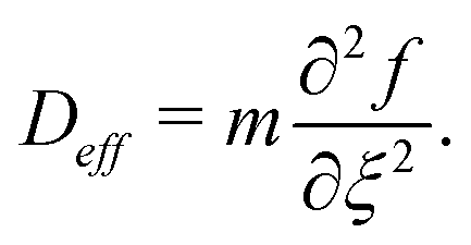
The driving force for spinodal decomposition can be measured by the effective diffusion coefficient Deff, which is related to the curvature of the free energy density at the global density:42| |  | (13) |
Fig. 3(b) shows that this curvature is significantly less negative in the density-dependent case than the density-independent case (comparing (ξ = 0.3, b = −0.5) and (ξ = 0.3, a = −1.0)). We therefore expect spinodal decomposition to happen more slowly for the density-dependent case. Indeed, Fig. 7(a) shows that this is the case; here we plot the maximum density ξmax in our simulations as a function of time following the quench to (ξ = 0.3, b = −0.5) or (ξ = 0.3, a = −1.0) for the density-dependent and -independent cases respectively. We can also measure the time taken to reach the condensed phase density ξcp, which is ∼1.75 in both cases: this time is indeed much shorter for the density-independent simulation (tps ∼ 550 SU versus tps ∼ 3750 SU in the density-dependent case); see also Movies S6 (density-independent) and S7 (density-dependent) in ESI.† From Fig. 7(b), which shows representative density distributions at tps of the density-dependent (∼3750 SU) and -independent systems (∼550 SU), we see that the density-dependent system contains a much larger proportion of the noncondensed phase at this early stage.
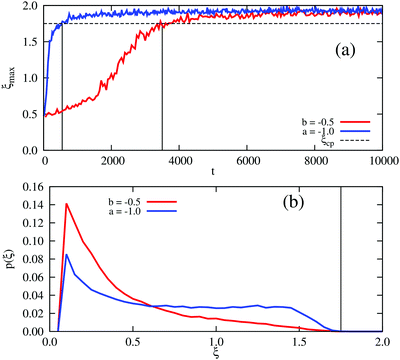 |
| | Fig. 7 Field simulations. Phase separation in the density-dependent system (red curves) is slower than in the density-independent system (blue curves). (a) Time evolution of the maximum density, ξmax. The dashed horizontal line corresponds to the phase separation density ξcp = 1.75, the location of the condensed phase peak in Fig. 5(a). Black vertical lines represent the time, tps, that it takes for the systems to reach ξcp. (b) The corresponding distribution of densities, p(ξ), at tps ∼ 3750 SU (density-dependence) and tps ∼ 550 SU (density-independence). The black vertical line corresponds to ξcp = 1.75. | |
Spatial structure during phase separation.
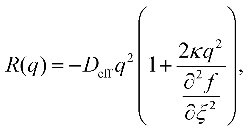
The length scale of the condensed phase structures formed during spinodal decomposition is controlled by the wavevector q at which the amplification factor| |  | (14) |
is maximal.42Eqn (14) shows that R(q) depends on the curvature of the free energy density; its maximum occurs at a smaller q-value in the density-dependent case than in the density-independent case (Fig. S12(a) (ESI†), comparing (ξ = 0.3, b = −0.5) and (ξ = 0.3, a = −1.0)). We therefore expect to see larger domains during spinodal decomposition for the density-dependent system. Indeed, Fig. 8 shows that there is a clear difference in the spatial structures that form during phase separation in the two systems. In the density-independent system, narrow elongated structures form that span the entire system before breaking up (Fig. 8(a)–(c)). In the density-dependent system, however, these elongated structures do not form; phase separation proceeds instead via the formation of larger, rounded aggregates (Fig. 8(d) and (e)). For both systems, at later times, t > tps, the aggregates grow via coarsening and coalescence with long-time scaling behaviour ∝t0.63 (see Fig. S12(b), ESI†); this is consistent with classical models of phase separation (∝t0.67) in diffusive systems with negligible hydrodynamic interactions.36
 |
| | Fig. 8 Field simulations. Simulation snap-shots showing the time evolution of the density-independent (a–c) and -dependent (d and e) systems during time tps. (a) Density-independent,  . (b) Density-independent, . (b) Density-independent,  . (c) Density-independent, t = 550 SU = 1tps. (d) Density-dependent, . (c) Density-independent, t = 550 SU = 1tps. (d) Density-dependent,  . (e) Density-dependent, . (e) Density-dependent,  . (f) Density-dependent, t = 3500 SU = 1tps. . (f) Density-dependent, t = 3500 SU = 1tps. | |
Local free-energy barrier in the spinodal regime for density-dependent interactions.
The characteristic features of phase separation in the spinodal regime of the density-dependent system – fewer small aggregates, narrower aggregate size distribution, slower phase separation and larger, more circular spatial domains at early times – can be rationalised in terms of the free energy barrier at low density (Fig. 3(a)), which arises from the low-density coexistence region of the phase diagram (Fig. 2(d)). This free energy barrier leads to a region of positive curvature of f versus ξ, and hence positive effective diffusion coefficient, for low ξ. Even when the system is quenched to a point within the spinodal regime, when local regions of low density form, these are in the coexistence region of the phase diagram (Fig. 2(d)) and hence they are locally “stable”, in the sense that the formation of higher density structures is hindered by the free-energy barrier. This contrasts with the density-independent case (also shown in Fig. 3(a)), for which a gas of monomers is always unstable to aggregation. The fact that such a free energy barrier can have significant effects even when the system is quenched into the spinodal regime is a consequence of the global conservation of the order parameter and gives rise to a weakly first order transition, whereas without global conservation of the order parameter, the first order transition would be more pronounced.
“System-swap” simulations confirm the role of thermodynamics.
Our discussion so far suggests that thermodynamics – i.e., the form of the free-energy density – is crucial in controlling the nature of phase separation in the density-dependent system. But to what extent does the history of a particular phase separation trajectory control its future behaviour? This question can be addressed by “switching” from a density-dependent free-energy function to a density-independent one (or vice versa), during a phase separation trajectory. If the controlling factor is indeed the free-energy density, then the trajectory should rapidly adjust its characteristics in line with the new free-energy function. If instead, trajectory history is important, then we would expect the trajectory to retain the characteristics of its original free-energy function.
To test this, we performed density-dependent simulations initialised with the configurations from density-independent simulations taken at tps (i.e., once the condensed phase density had been reached), and vice versa. Fig. 9 shows representative snapshots during the time evolution of these “switched” simulations (2nd and 4th rows), alongside, for comparison, representative snapshots from simulations (initiated from the same configurations) that were not switched (1st and 3rd rows). Rows 1 and 2 illustrate the effect of turning on density-dependent interactions in systems initialised from density-independent simulations. Shortly after switching (compare (b) and (e)), the density becomes redistributed in a manner that increases the concentration of the gas phase whilst lowering that of the dense phase (see also Fig. S13, ESI†). This redistribution persists at later times (see Fig. S13, ESI†), leading to smaller aggregates (compare (c) and (f)) that are more narrowly distributed in size (see Fig. S14, ESI†). In other words, the system takes on the characteristics of a density-dependent free-energy function.
 |
| | Fig. 9 Field simulations. Simulation snap-shots showing the time evolution of the “non-switched” (1st and 3rd row) vs. switched simulations (2nd and 4th row). 1st row (top) – density-independent simulation initialised with a configuration sampled from a density-independent simulation at time tps = 550 SU. 2nd row – density-dependent simulation initialised with a configuration sampled from a density-independent simulation at time tps = 550 SU. 3rd row – density-dependent simulation initialised with a configuration sampled from a density-dependent simulation at time tps = 3500 SU. 4th row (bottom) – density-independent simulation initialised with a configuration sampled from a density-dependent simulation at time tps = 3500 SU. Columns (a, d, g, j), (b, e, h, k), and (c, f, i, l) correspond to snapshots taken at times t = 0 SU, t = 1500 SU, and t = 50000 SU after initialisation. | |
Switching from density-dependent interactions to density-independent interactions (rows 3 and 4) has the opposite effect, i.e., the aggregates become less diffuse and the density is redistributed to decrease the gas-phase concentration whilst increasing that of the condensed phase aggregates; this behaviour persists at later times, leading to large aggregates that are more broadly distributed in size – i.e., the system takes on the characteristics of a density-independent free-energy function. Therefore we conclude that it is the underlying thermodynamics which govern the phase separation process; the trajectory history has little influence on the long term dynamics of phase-separation.
Particle-based model
To assess the generality of our observations, we also performed 2-dimensional particle-based Brownian dynamics simulations, with and without interactions that depend on the local particle density. In these simulations, particles interact via the cut and shifted Lennard-Jones potential. Although this potential is more commonly used in atomistic simulations, it has become a popular choice for modelling interactions between bacteria43–46 or between bacteria and polymers,24 since it captures the essential features of attraction and repulsion between soft-interacting particles. To implement a density-dependent cohesive interaction we modify the standard Lennard-Jones potential such that the parameter ε, which governs the strength of the attraction, depends on the local particle density ρ: ε = ε(ρ). The interaction potential then becomes| | | U(r,ρ) = 4ε(ρ)[(σ/r)12 − (σ/r)6 − Uc], | (15) |
for r < rc, and U = 0 for r ≥ rc, where r is the inter-particle distance. Here, σ is the particle diameter and the shift Uc = (σ/rc)12 − (σ/rc)6 ensures that U = 0 at the cut-off distance rc = 1.2σ.
Following eqn (5), ε(ρ) is assumed to take the linear form
where
ε′, which has units of energy times area, determines the sensitivity of the interaction to the particle density. Thus the strength of the interaction between any pair of particles increases with increasing local density of the surrounding particles (see the ESI
† for details). In practice, at each time step, the local density
ρ at each particle coordinate
x is computed on a grid and the corresponding value of
ε is assigned to that particle
viaeqn (16) (see the ESI
† for details). To compute interactions between pairs of particles with different local densities, and hence different values of
ε, we use the Lorentz–Berthelot rule

(see the ESI
† for details), where
ε1 and
ε2 are computed according to
eqn (16).
In this particle-based model, as in our field simulations, the total density is conserved, i.e., particles do not grow, reproduce or die. The particles are also assumed to be non-motile.
Particle-based simulations
We performed 2-dimensional BD simulations of N monodisperse discs interacting viaeqn (15) and (16), comparing our results to those of equivalent simulations with a standard, density-independent, Lennard-Jones potential (no ρ dependence in eqn (15)).
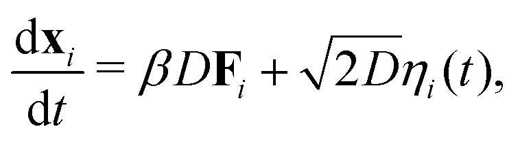
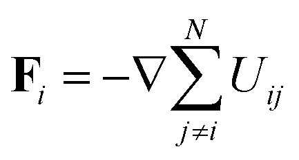
The position, xi of an individual particle, i, evolves in our simulations via numerical integration of the over-damped Langevin equation
| | 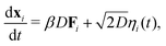 | (17) |
where
D is the diffusion coefficient,
β = 1/
kBT,

is the force on particle
i resulting from interactions with the other
N − 1 particles, and
ηi(
t) is a unit variance white noise variable with 〈
ηi(
t) 〉 = 0 and
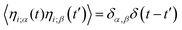
, with
α,
β =
x,
y. To implement our simulations, we non-dimensionalised
eqn (17) using
σ,
kBT, and

as the basic units of length, energy, and time respectively (see the ESI
† for details). Simulations were performed in a square box of length 115
σ with periodic boundary conditions, using the Euler method of numerical integration with a time-step of 2.5 × 10
−5τ.
To characterise the system with density-dependent interactions, we systematically varied the interaction strength parameter, ε′, for three values of the total number of particles: N = 3600, corresponding to area fraction θ = 0.21, N = 4900 (θ = 0.29), and N = 6400 (θ = 0.38).47 We observed similar phase separation behaviour in all three systems – we therefore focus on the results for the intermediate area fraction θ = 0.29 (N = 4900). Results for the other area fractions can be found in ESI.†
After an equilibration period (1000 τ) without inter-particle attractions, our simulations were run for times trun = 1250 τ (in total 2250 τ), which is the approximate time required for the fraction of particles in the condensed phase to reach a steady state. After time trun, coarsening and coalescence change the distribution of aggregate sizes (ultimately leading to the formation of one large phase-separated domain), but the aggregated fraction remains constant (see the ESI† for details). The time-scales used here, although not long enough to observe fully phase separated states, are long enough to capture the rich early aggregation behaviour resulting from density-dependent cohesion.
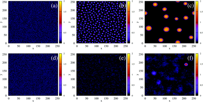
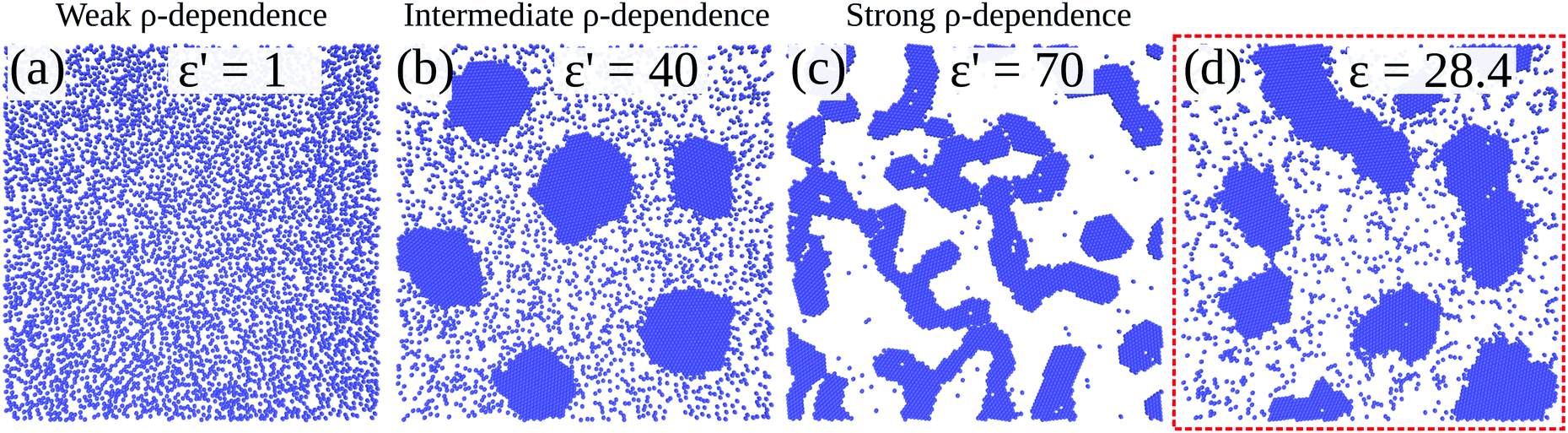
Fig. 10 shows configurations of the system for θ = 0.29 and for various values of ε′, after simulation time trun = 1250τ. For ε′ = 1 (weak density-dependent attraction), the system is in a “gas-like” phase (Fig. 10(a)) whose ordering, characterised by the structure factor S(q), is consistent with that of a simple colloidal dispersion or hard sphere fluid (see the ESI† for details). For ε′ = 70 (strong density-dependent attraction), elongated and interconnected aggregates give rise to a “gel-like” state (Fig. 10(c)).
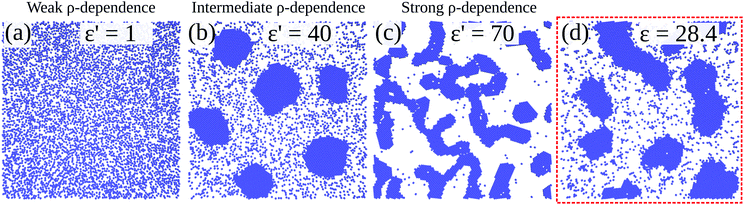 |
| | Fig. 10 Particle-based simulations. Simulation snapshots of our particle-based simulations, for area fraction θ = 0.29. Snapshots are taken at time trun = 1250 τ. Panels (a)–(c) show results from systems with a density-dependent potential (for different values of ε′, in units of kBTσ2); panel (d) (red box) shows a snapshot from a system with a density-independent potential (with ε in units of kBT). | |
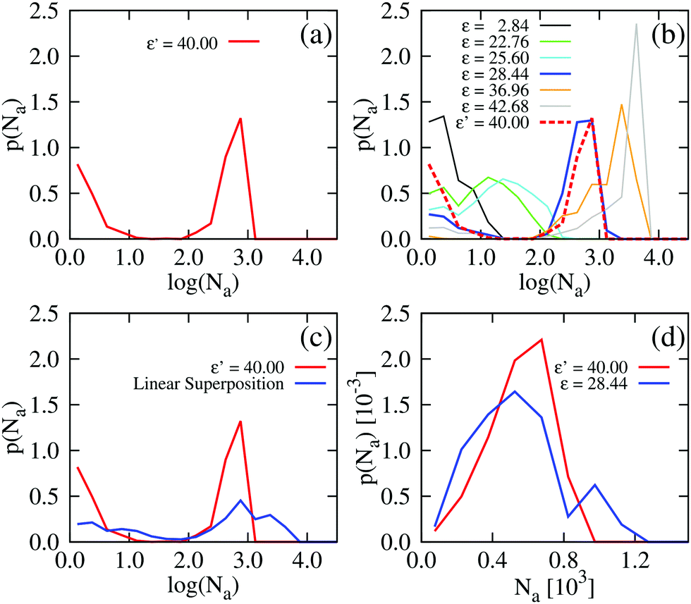
For ε′ = 40 (intermediate density-dependent attraction), we obtain interesting behaviour arising from the density-dependent attraction. Our simulation snapshots at trun = 1250τ (Fig. 10(b)) show clearly that the system is undergoing phase separation into condensed and non-condensed phases, with the emergence of the former being confirmed by the presence of well-defined peaks in S(q) (see the ESI† for details). For this value of ε′, inspection of the simulation trajectory shows that phase separation proceeds via the formation of aggregates that appear to grow only once they reach a threshold size (see Movie S8 in ESI†). This is reminiscent of the “spinodal nucleation” phenomenon observed in our field simulations. Fig. 11(a) shows the aggregate size distribution for ε′ = 40, computed at time trun (i.e., the probability that a particle belongs to an aggregate of a given size). Consistent with the snapshot of Fig. 10(b), the distribution is bimodal, with two peaks corresponding to aggregates of >300 particles and individual particles (clusters of <2 particles).
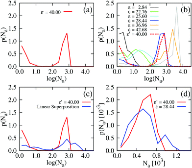 |
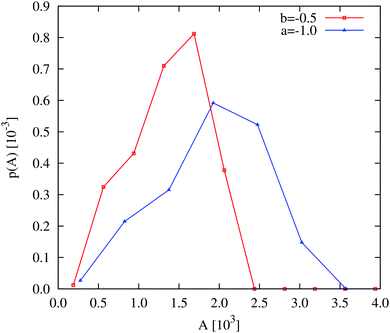
| | Fig. 11 Particle-based simulations. Aggregate size distributions, computed at trun = 1250τ, for density-dependent and -independent systems with area fraction θ = 0.29. The distributions are weighted by the aggregate size, Na, such that they represent the probability p(Na) that a particle belongs to an aggregate of size Na particles. In plots (a) to (c), the distributions are plotted vs. the logarithm of Na. All distributions were generated from 10 final configurations at trun = 1250τ generated in independent replicate simulations. ε′ values are in units of kBTσ2 and ε values are in units of kBT. Aggregate sizes were computed using a linked-list method.48 (a) p(Na) for the density-dependent system with ε′ =40. (b) p(Na) for density-independent systems with ε values in the range ε = 2.84 → 42.68 that is explored in a density-dependent simulation with  . Note that the apparent peaks located in the range 1 < log(Na) < 2.0 (green and cyan curves) correspond to transient aggregates, i.e., aggregate “seeds” which dissolve soon after formation. For comparison, the red curve shows p(Na) for the density-dependent system with ε′ = 40. (c) A weighted linear superposition (blue curve) of the p(Na) curves computed in the density-independent simulations of (b) (see the ESI† for details). Again, the red curve shows p(Na) for the density-dependent system with ε′ = 40. (d) Aggregate size distribution, including only aggregates of size Na > 10 particles, for ε = 28.44 (density-independent) and ε′ = 40 (density-dependent). . Note that the apparent peaks located in the range 1 < log(Na) < 2.0 (green and cyan curves) correspond to transient aggregates, i.e., aggregate “seeds” which dissolve soon after formation. For comparison, the red curve shows p(Na) for the density-dependent system with ε′ = 40. (c) A weighted linear superposition (blue curve) of the p(Na) curves computed in the density-independent simulations of (b) (see the ESI† for details). Again, the red curve shows p(Na) for the density-dependent system with ε′ = 40. (d) Aggregate size distribution, including only aggregates of size Na > 10 particles, for ε = 28.44 (density-independent) and ε′ = 40 (density-dependent). | |
To determine whether this behaviour is intrinsic to the density-dependent interaction potential, we also performed a series of simulations with a standard, density-independent, Lennard-Jones interaction potential. We used values of the interaction strength ε in the range 2.84 → 42.68 kBT: this corresponds to the ε-range that is sampled (viaeqn (16)) in the final configuration of our density-dependent simulation with ε′ = 40 (see the ESI† for details). A snapshot from the density-independent simulation with ε = 28.4 kBT is shown in Fig. 10(d). Consistent with our observations from the field simulations, the aggregates are more varied in size and shape than those of the density-dependent system, and the non-condensed phase contains small clusters rather than single particles (compare to Fig. 10(b)). Phase separation in this system proceeds in a manner typical of spinodal decomposition, in that clusters form rapidly throughout the entire system (see Movie S9 in ESI†). Fig. 11(b) shows the aggregate size distribution (at time trun) for density-independent simulations with ε = 2.84 → 42.68 (see also the ESI†). In contrast to the density-dependent case, none of these distributions are bimodal. Rather, the density-independent system forms either large aggregates (for ε > 25.6), or predominantly small aggregates (for ε ≤ 25.6). We also checked that a weighted linear superposition of the aggregate size distributions for different ε values cannot reproduce the aggregate size distribution produced by the density-dependent simulations (Fig. 11(c)) (see the ESI† for details). Thus, as we observed in our field simulations, the bimodal aggregate size distribution appears to be an intrinsic feature of the density-dependent system. For the particle-based simulations, we also observe that the peaks in the aggregate size distribution are broader for the density-independent simulations than in the density-dependent case (Fig. 11(b); see also Fig. 11(d) which confirms that the large-aggregate peak is narrower in the density-dependent system). Thus, density-dependent aggregation appears to confer increased “control” of aggregate size.
Given that our particle-based simulations exhibit qualitatively similar behaviour to that of our field simulations, we can conclude that “spinodal-nucleation”-like cluster formation, consisting of rather homogeneous aggregates that appear to show a barrier to growth, bimodal aggregate size distribution and a narrow cluster size distribution, are characteristic of systems with density-dependent attractive interactions, whether manifested as a cubic term in the Landau–Ginzburg free energy, or as a density-dependent potential in a particle-based model.
Conclusions
Living cells often interact via secreted molecules, some of which can affect inter-cellular mechanical interactions. In this paper, we have shown that in an idealised model where the secreted cohesive agent is degraded rapidly enough that their concentration profile around each cell reaches a steady state, the effects of the secreted agent can be coarse-grained as an attractive interaction between cells that depends on the local cell density. This in turn leads to a picture in which cell aggregation can be thought of as a phase separation process driven by density-dependent attractive interactions – a process which turns out to differ in interesting ways from phase separation in standard, “density-independent” systems. Our results complement previous work on systems where phase separation is driven by particle motility,19,21–24,26 on changes in particle motility due to polymer secretion,49 and on bacterial aggregation driven by addition of exogenous polymer.24,28–32
Combining a field theory approach with particle-based simulations, we observe behaviour that appears to be characteristic of systems with density-dependent attractive interactions. Specifically, we see an apparent barrier to cluster growth even in the spinodal regime, that we term “spinodal nucleation”, and bimodal aggregate size distributions with narrow peaks – corresponding to aggregates of rather uniform size in a “sea” of single particles. These characteristic behaviours can be understood as originating from a local free-energy barrier to cluster formation at low particle density, even in the spinodal region of the phase diagram. This barrier arises because local density fluctuations drive the system into the low-density coexistence region of the phase diagram, which in turn exists as a consequence of the cubic term that emerges from the Landau–Ginzburg free energy when the secretion of cohesion-inducing agents are considered, like that observed in nematic liquid crystals.39
From the point of view of real biological cells, our model is highly simplified: we neglect, for example, cell motility, proliferation and death. Moreover, our assumption that the concentration field of cohesive agent is at steady state around a given particle is idealistic: in reality cohesive agents such as extracellular polymers are likely to degrade only slowly and may well accumulate in the system. Even for rapidly degrading agents the concentration field might be perturbed, for example by local fluid motion. Taking account of these factors would of course require a different modelling approach. Nevertheless, our work suggests that production of cohesive molecules might provide a route to control of aggregate size, and reveals interesting physics associated with the kind of density-dependent interactions that could be generated by the non-equilibrium process of cohesive agent production.
Conflicts of interest
There are no conflicts of interest to declare.
Acknowledgements
G. M. thanks Joakim Stenhammar and Kasper Kragh for helpful discussions in the early stages of this project and gratefully acknowledges financial support from both the EPSRC (Grant No. EP/J007404) and the HFSP (Grant No. RGY0081/2012). R. A. was supported by a Royal Society University Research Fellowship and by the ERC under grant 682237 “EVOSTRUC”. D. M. was supported by the ERC grant 648050 “THREEDCELLPHYSICS”. This work was supported by the Biotechnology and Biological Sciences Research Council (BB/R012415/1).
References
- M. B. Miller and B. L. Bassler, Annu. Rev. Microbiol., 2001, 55, 165–199 CrossRef CAS.
- C. M. Waters and B. L. Bassler, Annu. Rev. Cell Dev. Biol., 2005, 21, 319 CrossRef CAS PubMed.
- L. Laganenka, R. Colin and V. Sourjik, Nat. Commun., 2016, 7, 12984 CrossRef CAS PubMed.
- C. Frantz, K. M. Stewart and V. M. Weaver, J. Cell. Sci., 2010, 123, 4195–4200 CrossRef CAS PubMed.
- M. Takeichi, Science, 1991, 251, 1451–1455 CrossRef CAS PubMed.
- A. Konovalova, T. Petters and L. Søgaard-Andersen, FEMS Microbiol. Rev., 2010, 34, 89–106 CrossRef CAS PubMed.
- H. C. Flemming, T. R. Neu and D. J. Wozniak, J. Bacteriol., 2007, 189, 7945–7947 CrossRef CAS PubMed.
- H.-C. Flemming and J. Wingender, Nat. Rev. Microbiol., 2010, 8, 623–633 CrossRef CAS PubMed.
- D. Schleheck, N. Barraud, J. Klebensberger, J. S. Webb, D. McDougald, S. A. Rice and S. Kjelleberg, PLoS One, 2009, 4, 1–15 CrossRef PubMed.
- M. Alhede, K. N. Kragh, K. Qvortrup, M. Allesen-Holm, M. van Gennip, L. D. Christensen, P. S. Jensen, A. K. Nielsen, M. Parsek, D. Wozniak, S. Molin, T. Tolker-Nielsen, N. Høiby, M. Givskov and T. Bjarnsholt, PLoS One, 2011, 6, 1–12 CrossRef PubMed.
- K. N. Kragh, J. B. Hutchison, G. Melaugh, C. Rodesney, A. E. L. Roberts, Y. Irie, P. Jensen, S. P. Diggle, R. J. Allen, V. Gordon and T. Bjarnsholt, mBio, 2016, 7, e00237 CrossRef CAS PubMed.
-
S. Wuertz, P. Bishop and P. Wilderer, Biofilms in Wastewater Treatment, IWA Publishing, 2003 Search PubMed.
- C. Kumar and S. Anand, Int. J. Food Microbiol., 1998, 42, 9–27 CrossRef CAS PubMed.
- T. Bjarnsholt, P. O. Jensen, M. J. Fiandaca, J. Pedersen, C. R. Hansen, C. B. Andersen, T. Pressler, M. Givskov and N. Hoiby, Pediatr. Pulmonol., 2009, 44, 547–558 CrossRef PubMed.
- T. Bjarnsholt, M. Alhede, M. Alhede, S. R. Eickhardt-Sørensen, C. Moser, M. Kühl, P. Østrup Jensen and N. Høiby, Trends Microbiol., 2013, 21, 466–474 CrossRef CAS PubMed.
- B. J. Staudinger, J. F. Muller, S. Halldórsson, B. Boles, A. Angermeyer, D. Nguyen, H. Rosen, L. Baldursson, M. Gottfresson, G. H. Gumundsson and P. K. Singh, Am. J. Respir. Crit. Care Med., 2014, 189, 812–824 CrossRef CAS PubMed.
- K. N. Kragh, M. Alhede, M. Rybtke, C. Stavnsberg, P. Ø. Jensen, T. Tolker-Nielsen, M. Whiteley and T. Bjarnsholt, Appl. Environ. Microbiol., 2018, 84, e02264 Search PubMed.
- S. Ramaswamy, Annu. Rev. Condens. Matter Phys., 2010, 323–345 CrossRef.
- M. E. Cates and J. Tailleur, Ann. Rev. Condend. Matter Phys., 2015, 6, 219–244 CrossRef CAS.
- R. Romanczuk, M. Bär, W. Ebeling, B. Lindner and L. Schimansky-Geier, EPL, 2012, 202, 1–162 Search PubMed.
- J. Stenhammar, A. Tiribocchi, R. J. Allen, D. Marenduzzo and M. E. Cates, Phys. Rev. Lett., 2013, 145702 CrossRef PubMed.
- M. C. Marchetti, J. F. Joanny, S. Ramaswamy, T. B. Liverpool, J. Prost, M. Rao and R. A. Simha, Rev. Mod. Phys., 2013, 85, 1143–1189 CrossRef CAS.
- G. S. Redner, M. F. Hagan and A. Baskaran, Phys. Rev. Lett., 2013, 110, 055701 CrossRef PubMed.
- J. Schwarz-Linek, C. Valeriani, A. Cacciuto, M. E. Cates, D. Marenduzzo, A. N. Morozov and W. C. K. Poon, Proc. Natl. Acad. Sci. U. S. A., 2012, 109, 4052–4057 CrossRef CAS PubMed.
- J. R. Howse, R. A. L. Jones, A. J. Ryan, T. Gough, R. Vafabakhsh and R. Golestanian, Phys. Rev. Lett., 2007, 99, 048102 CrossRef PubMed.
- A. Doostmohammadi, S. P. Thampi and J. M. Yeomans, Phys. Rev. Lett., 2016, 117, 048102 CrossRef PubMed.
- J. Stenhammar, C. Nardini, R. W. Nash, D. Marenduzzo and A. Morozov, Phys. Rev. Lett., 2017, 119, 028005 CrossRef PubMed.
- G. Dorken, G. P. Ferguson, C. E. French and W. C. K. Poon, J. R. Soc., Interface, 2012, 9, 3490–3502 CrossRef PubMed.
- J. Schwarz-Linek, G. Dorken, A. Winkler, L. G. Wilson, N. T. Pham, C. E. French, T. Schilling and W. C. K. Poon, EPL, 2010, 89, 68003 CrossRef.
- P. R. Secor, L. A. Michaels, A. Ratjen, L. K. Jennings and P. K. Singh, Proc. Natl. Acad. Sci. U. S. A., 2018, 115, 10780–10785 CrossRef CAS PubMed.
-
H. Lekkerkerker and R. Tuinier, Colloids and the Depletion Interaction, Springer Netherlands, 2011 Search PubMed.
- S. Biggs, M. Habgood, G. J. Jameson and Y. de Yan, Chem. Eng. J., 2000, 80, 13–22 CrossRef CAS.
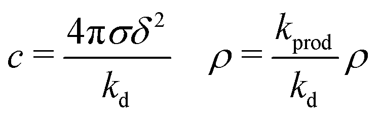
-
We note that relation (5) can be expressed more simply if the cohesion-inducing agent is degraded on a much slower timescale than it takes for it to diffuse the radius of the particle, such that
 . In this case we obtain the simple result that
where kprod ≡ 4πσδ2 is the net production rate of cohesion-inducing agents, per particle. To get an idea of the absolute value of the degradation rate that is implied for the condition  to hold, let us suppose the cohesion-inducing agent has a radius, R = 0.1 μm, which is approximately 10 times smaller than that of a typical bacterium or colloidal particle (∼1 μm). The diffusion constant of the agent can be computed from the Stokes–Einstein relation D = kBT/6πγR. At 25 °C in water, the product of the Boltzmann constant, kB, and temperature, T, is 4 × 10⁻²¹ J, and the dynamic viscosity, γ = 9 × 10⁻⁴ Pa s, which then gives D = 2.4 × 10⁻¹² μm2 s−1. For the condition
  , degradation is required to happen at a rate 2.4 × 10⁻² s−1, which translates to a typical lifetime for a cohesion-inducing agent of 4 minutes
.
, degradation is required to happen at a rate 2.4 × 10⁻² s−1, which translates to a typical lifetime for a cohesion-inducing agent of 4 minutes
.
- A. A. Louis, J. Phys.: Condens. Matter, 2002, 14, 9187–9206 CrossRef CAS.
- I. Pagonabarraga and D. Frenkel, Mol. Simul., 2000, 25, 167–175 CrossRef CAS.
-
P. M. Chaikin and T. C. Lubensky, Principles of condensed matter physics, Cambridge University Press, 1995 Search PubMed.
-
M. Plischke and B. Bergersen, Equilibrium Statistical Physics, World Scientific, 2006 Search PubMed.
- P. C. Hohenberg and B. I. Halperin, Rev. Mod. Phys., 1977, 49, 435–479 CrossRef CAS.
-
P. G. de Gennes and J. Prost, The Physics of Liquid Crystals, Clarendon Press, 1995 Search PubMed.
- J. W. Cahn and J. E. Hilliard, J. Chem. Phys., 1958, 28, 258 CrossRef CAS.
- Note that this choice breaks the fluctuation–dissipation theorem (FDT) linking noise strength and mobility, however given the dynamics of polymer secretion outlined in eqn (1)–(5), this is acceptable as the
system will typically be out of equilibrium. That said, however, we repeated several of our simulations with FDT restored, and found qualitatively similar behaviour to that presented in the main manuscript (see the ESI† for details).
-
R. A. L. Jones, Soft Condensed Matter, Oxford University Press, 2002 Search PubMed.
- M. Abkenar, K. Marx, T. Auth and G. Gompper, Phys. Rev. E: Stat., Nonlinear, Soft Matter Phys., 2013, 88, 062314 CrossRef PubMed.
- S. D. Ryan, A. Sokolov, L. Berlyand and I. S. Aranson, New J. Phys., 2013, 15, 105021 CrossRef PubMed.
- S. Ryan, L. Berlyand, B. Haines and D. Karpeev, Multiscale Model. Simul., 2013, 11, 1176–1196 CrossRef.
- V. Prymidis, H. Sielcken and L. Filion, Soft Matter, 2015, 11, 4158–4166 RSC.
- Note that computing a full phase diagram, as we did for the field simulations, would be a computationally intensive task in our particle-based model.
- S. Stoddard, J. Comput. Phys., 1978, 27, 291–293 CrossRef.
- C. Valeriani, R. J. Allen and D. Marenduzzo, J. Chem. Phys., 2010, 132, 204904 CrossRef CAS PubMed.
Footnote |
| † Electronic supplementary information (ESI) available: For movies, and details on simulation methods, systems at different area fraction, structure factors, and phase diagrams for continuum model. See DOI: 10.1039/c9sm01462d |
|
| This journal is © The Royal Society of Chemistry 2019 |
Click here to see how this site uses Cookies. View our privacy policy here. 
 Open Access Article
 This Open Access Article is licensed under a Creative Commons Attribution-Non Commercial 3.0 Unported Licence
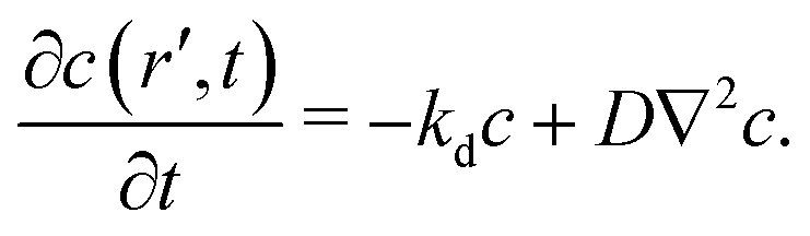


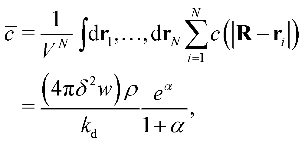
 . The ratio α compares the timescale for the cohesion-inducing agent to diffuse the size of the source particle, to the timescale of its degradation, and is assumed to be small in our steady-state regime.33 With this is mind, eqn (5) shows that the concentration of cohesion-inducing agents is a linear function of the particle number density ρ,33 and therefore we can expect cohesive interactions, which are mediated by these agents, to be a linear function of the local particle density (provided we are in the regime where the agent concentration can be considered to be in steady state). We also note that 4πδ2w is the total amount of agent being secreted through the surface per unit time, and thus the prefactor in eqn (5) is the ratio of the production rate to the degradation rate.
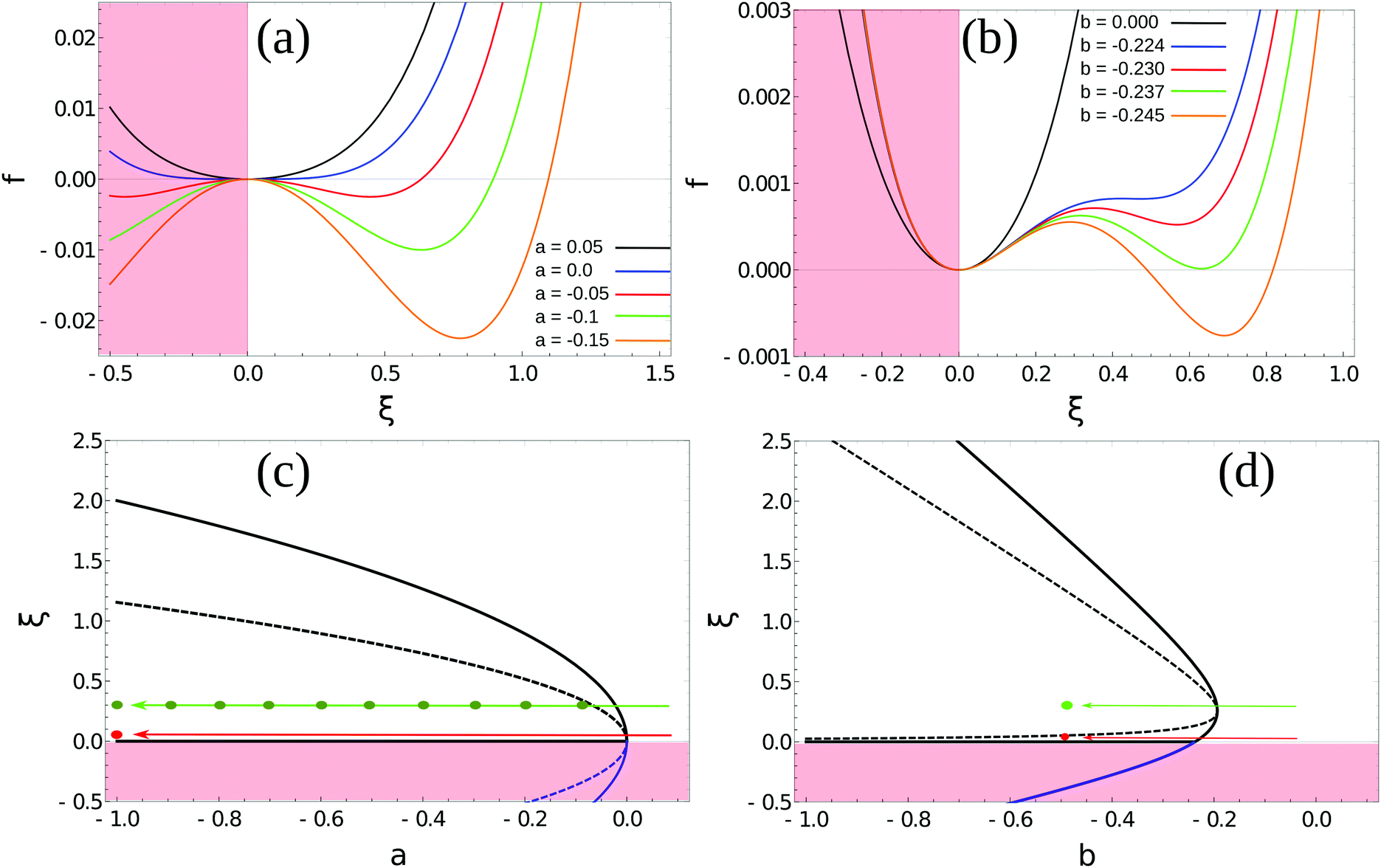
 . For the model represented by eqn (6) to be physically realistic, the condition of positive density, ξ ≥ 0, has to be imposed throughout, ruling out any equilibrium phase with ξ < 0. Fig. 2(a) shows the homogeneous part of the free energy density (eqn (6)); the region shaded red is inaccessible because it does not meet the condition ξ ≥ 0. The continuous transition from a state whereby ξ = 0 is the global minimum of the free energy density to a state where the global minimum is a positive finite value,
 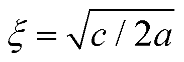 , is a signature of the fact that this free energy density would produce a second-order phase transition in a system where the order parameter is not globally conserved.
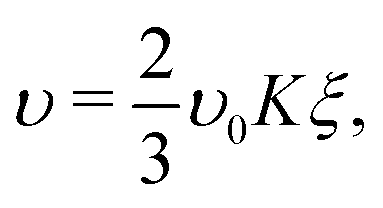
 , where ξ0 is the overall system density and A is the total area), the phase-separation dynamics of the two systems can be modelled using the Cahn–Hilliard equation40
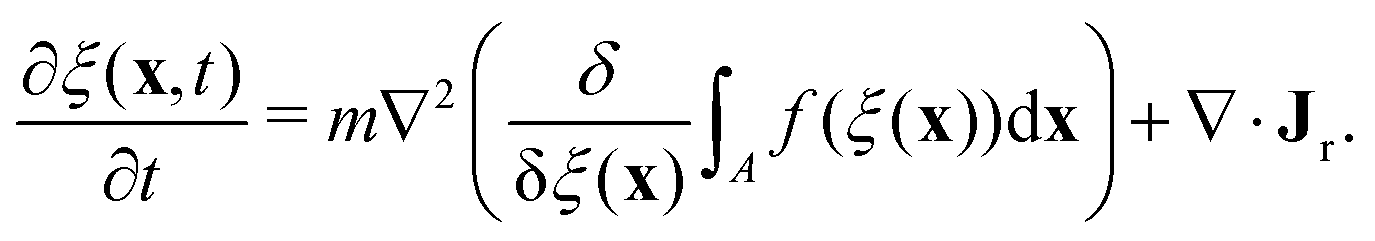
 , with α,β = x, y. For simplicity, both m and the random noise strength Λ were kept constant, at m = 0.01 and Λ = 0.1.41Eqn (12) was solved on a 256 × 256 grid using standard finite difference simulations, with periodic boundary conditions.

 . (b) Density-independent,
 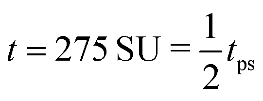 . (c) Density-independent, t = 550 SU = 1tps. (d) Density-dependent,
 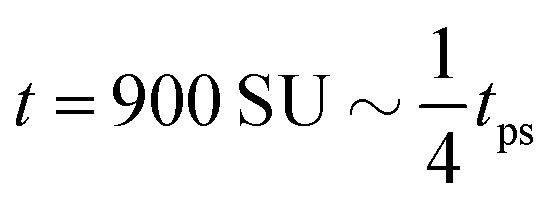 . (e) Density-dependent,
  . (f) Density-dependent, t = 3500 SU = 1tps.
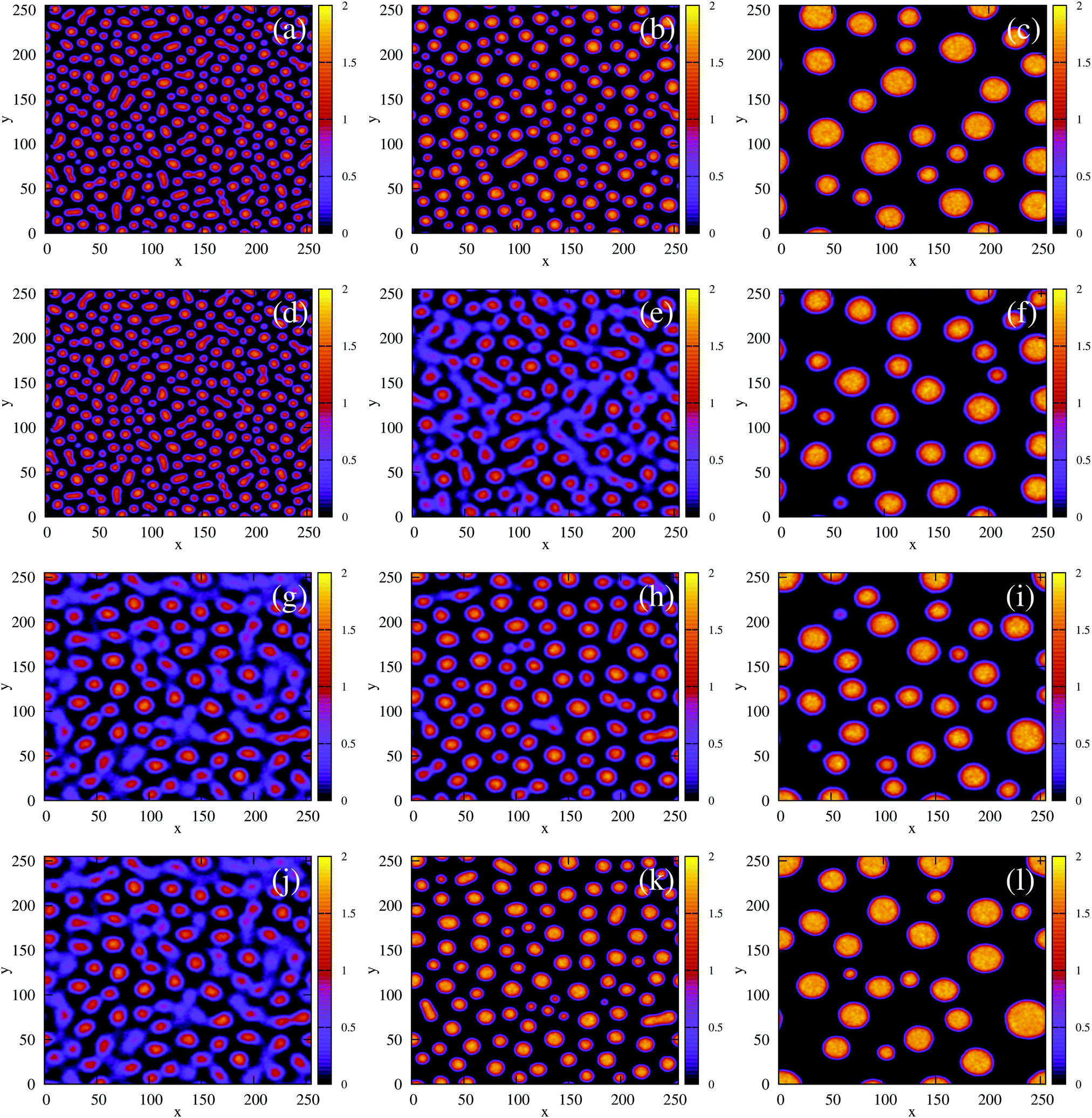
 (see the ESI† for details), where ε1 and ε2 are computed according to eqn (16).
 is the force on particle i resulting from interactions with the other N − 1 particles, and ηi(t) is a unit variance white noise variable with 〈ηi(t) 〉 = 0 and
 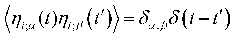 , with α,β = x,y. To implement our simulations, we non-dimensionalised eqn (17) using σ, kBT, and
 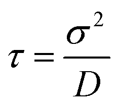 as the basic units of length, energy, and time respectively (see the ESI† for details). Simulations were performed in a square box of length 115 σ with periodic boundary conditions, using the Euler method of numerical integration with a time-step of 2.5 × 10⁻⁵τ.
 . Note that the apparent peaks located in the range 1 < log(Na) < 2.0 (green and cyan curves) correspond to transient aggregates, i.e., aggregate “seeds” which dissolve soon after formation. For comparison, the red curve shows p(Na) for the density-dependent system with ε′ = 40. (c) A weighted linear superposition (blue curve) of the p(Na) curves computed in the density-independent simulations of (b) (see the ESI† for details). Again, the red curve shows p(Na) for the density-dependent system with ε′ = 40. (d) Aggregate size distribution, including only aggregates of size Na > 10 particles, for ε = 28.44 (density-independent) and ε′ = 40 (density-dependent).