
 Open Access Article
 This Open Access Article is licensed under a Creative Commons Attribution-Non Commercial 3.0 Unported Licence
Sedimenting pairs of elastic microfilaments†
Marek
Bukowicki
and
Maria L.
Ekiel-Jeżewska
 *
*
Institute of Fundamental Technological Research, Polish Academy of Sciences, ul. Pawińskiego 5B, 02-106 Warsaw, Poland. E-mail: mekiel@ippt.pan.pl
First published on 11th October 2019
Abstract
The dynamics of two identical elastic filaments settling under gravity in a viscous fluid in the low Reynolds number regime is investigated numerically. A large family of initial configurations symmetric with respect to a vertical plane is considered, as well as their non-symmetric perturbations. The behaviour of the filaments is primarily governed by the elasto-gravitational number, which depends on the filament's length and flexibility, and the strength of the external force. Flexible filaments usually converge toward horizontal and parallel orientation. We explain this phenomenon and show that it occurs also for curved rigid particles of similar shapes. Once aligned, the two fibres either converge toward a stationary, flexibility-dependent distance, or tend to collide or continuously repel each other. Rigid and straight rods perform periodic motions while settling down. Apart from very stiff particles, the dynamics is robust to non-symmetric perturbations.
1 Introduction
Recently, there has been a growing interest in understanding basic features of the dynamics of elastic micro and nano filaments in water-based fluids, moving under a constant force or entrained by an ambient fluid flow. The motivation comes from modern research on modelling biological systems, such as bacteria,1,2 actin3–5 or nematodes,6,7 design of medical applications, e.g. hydrogel micro and nano fibers8–11 to deliver drugs, and investigations important to protect the environment, for example, waste-water treatment12 or diatom chains in oceans.13–17Systems of elastic filaments moving in fluids exhibit interesting, complex mechanical properties,18,19 caused by hydrodynamic interactions between segments of a single or multiple filaments. It is of special interest to investigate how elasticity affects sedimentation. The dynamics and shape deformation of single elastic filaments settling under gravity (or in a centrifuge) have been extensively studied numerically and experimentally.20–25 The motion of rigid elongated particles of different shapes26,27 can serve as a useful comparison. Sedimentation of pairs of rigid particles with complex shapes has been also studied.28–30 There exist also some numerical results on the dynamics of two and three elastic filaments.31,32 They indicate that the influence of elasticity on pairwise hydrodynamic interactions is a complex problem, still to be explored.
Therefore, the goal of this paper is to study the dynamics and shape deformation of pairs of elastic filaments settling under gravity and to check if they attract or repel each other, or tend to a stationary configuration, and how they orient with respect to gravity and to each other, depending on their elastic properties.
A good starting point (and a relevant reference) is the periodic dynamics of rigid elongated particles sedimenting in a vertical plane. The motion of spheroids was analyzed in ref. 33–35 and periodic orbits of spheroids were found with positions symmetric under reflection with respect to a perpendicular vertical plane.34–36 These solutions have been later used as a benchmark for different computational methods. In particular, a comparison with the Stokesian dynamics of particles made of spherical beads was performed.37,38 Similar symmetric periodic orbits of two elongated particles have been also found using the slender body approximation and the 3D lattice Boltzmann method for spherocylinders in a cubic periodic box.39 In this reference, the fluid velocity field around the sedimenting particles has also been analyzed.
Periodic dynamics of two identical rigid particles sedimenting in a vertical plane in a symmetric configuration have been observed and studied both numerically and experimentally for different shapes. Periodic trajectories of rigid ellipsoids were evaluated by Kim,34,35 and periodic motion of disks was measured and modeled theoretically by Chajwa et al.40 A variety of shapes were considered by Jung et al.41 who found periodic orbits in experiments with rods, disks, hemispheres and cubes, and in simulations of prolate and oblate spheroids. Moreover, similar orbits have been found also for larger numbers of rigid rods in symmetric configurations.39,42
In this paper, we will show that this important benchmark quasi-2D periodic solution can be generalized for a family of three-dimensional periodic motions of two filaments in configurations symmetric with respect to a vertical plane. In Section 2, the system and methodology will be described. In Section 3, we will demonstrate characteristic features of the periodic orbits for two rigid rods made of spherical beads, in the symmetric configurations.
In Section 4, we will move on to the analysis of two elastic filaments, initially in the same symmetric configuration as the rigid ones. We will investigate their complex dynamics, depending on the filament flexibility. In Section 5, the results will be compared with the dynamics of curved rigid filaments. Section 6 contains the results for slightly non-symmetric initial configurations. Finally, Section 7 is devoted to discussion and final conclusions.
2 System, methodology and notation
In this paper we investigate the dynamics of two identical flexible filaments or two rigid rods sedimenting at low Reynolds number. Particles are assumed to be non Brownian. We mainly focus on the configurations of particles symmetric with respect to reflection in a vertical plane x = 0 (as shown in Fig. 1), yet slightly non-symmetric cases are also considered. | ||
| Fig. 1 System and notation. Left panel: Initially the filaments are straight and horizontal; their configuration is described with the rotation angle φ(0) and the distance from the center-of-mass to the symmetry plane xcm(0). Right panel: Filaments can bend while sedimenting. Their ‘orientation’ is defined as the orientation of the end-to-end vector, which connects the centers of the first and the last bead in the filament. The time-dependent orientation of the end-to-end vector is given in spherical coordinates as the tilt angle θ(t) and the rotation angle φ(t). | ||
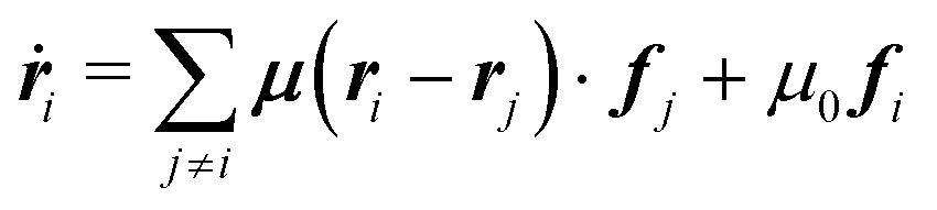
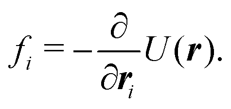
Each particle is represented as a chain of N connected beads and the dynamics of each bead is calculated. In our notation the positions of all bead centers constitute a vector r = (r1, r2,…, r2N) where ri denotes the position of the i-th bead. All beads are identical and have radii equal to a. The simulations are performed as Stokesian dynamics. In this approximation, inertia effects are neglected and non-hydrodynamic forces are balanced by the hydrodynamic ones. The particle velocities are proportional to the non-hydrodynamic forces acting on each bead: (1) gravitational force (corrected for buoyancy) and (2) elastic forces, calculated from the potential energy U(r) described in the next paragraph. The velocity of each bead i is the sum of contributions coming from the forces on all the other beads j ≠ i and the force acting on the bead i,
 | (1) |
 | (2) |
The gravity to elasticity ratio is characterized by dimensionless elasto-gravitational number B:25,31,32
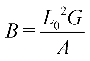 | (3) |
 | (4) |
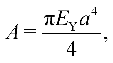
The elastic potential is given by:
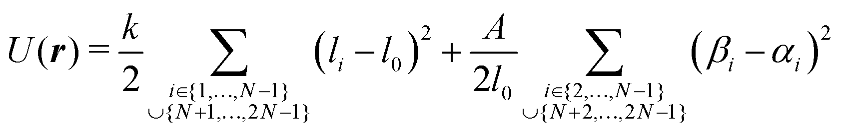 | (5) |
 | (6) |
 | (7) |
In summary, the model of elastic filaments presented here is the same as in our previous work.45 It is based on the harmonic elastic potential, similarly to work by Gruziel et al.46 Unlike in the latter reference, here the stiffness coefficients parameters k and A are coupled and very short range repulsion forces are absent. This elastic model is also similar to that in work by Schlagberger and Netz,21 Gauger and Stark47 and Marchetti et al.25 but with a harmonic bending potential instead of the ‘cosine’ one. Our choice is motivated by possible spurious effects of the ‘cosine’ potential in some circumstances.45
The dynamics of the system, i.e. the time-dependent positions of the beads, is determined by solving the system of first order autonomous ordinary differential equations given by eqn (1). The dynamics were calculated with the LSODA routine (ODEPACK Fortran 77 wrapped in Python), which automatically switches between non-stiff and stiff solvers with an adaptive time step.
Throughout the article we use dimensionless variables. Distances are normalized by the equilibrium length of the particle L0, forces are normalized by the gravitational force acting on a single particle, G, and the unit of time is given by 8πηL02/G, where η is the fluid viscosity. From now on all values will be given in dimensionless units, while any dimensional value will be marked with the tilde symbol above it.
Alongside vector r, which carries full information about bead positions, in this paper we use the positions of filament centers and orientations of end-to-end vectors to describe the main features of filament configurations in a concise form. The center of a filament is defined as the position of its center of mass: for the first, ‘right’ particle (whose x coordinates are greater than 0): 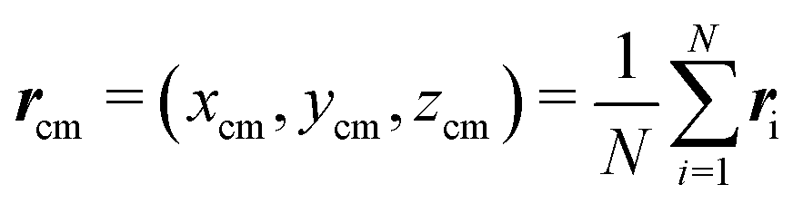 , and for the second, ‘left’ particle
 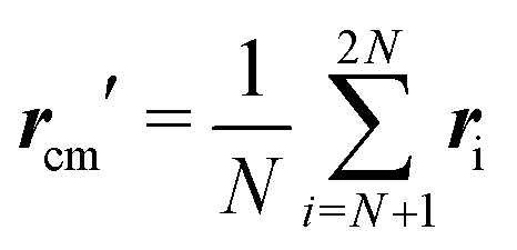 . An end-to-end vector connects the center of the first with the center of the last bead of a particle and its orientation is parametrized by angles θ and φ (see Fig. 1), which are defined in a manner consistent with the standard labeling in the spherical coordinate system.
The majority of the results presented in this paper are obtained for the system of two filaments symmetric with respect to reflection in a vertical plane.‡ In this case it is sufficient to consider the position and orientation of the ‘right’ particle. For systems where the symmetry is not imposed, the configuration of the ‘left’ particle has to be considered separately.
The main family of initial configurations is shown schematically in Fig. 1: the particles are located symmetrically in a horizontal plane. The vertical symmetry plane is located at x = 0. The filaments are straight and the distances between beads are equal to the equilibrium length of the bonds l0. Each initial configuration is given by the distance xcm(0) of the particle's center from the symmetry plane and the initial orientation angle φ(0). Other coordinates are set to: ycm(0) = 0, zcm(0) = 0, and θ(0) = π/2.
3 Periodic motion of rigid rods
First, let us briefly recapitulate the dynamics of rods which lie and move in the vertical plane, as shown in the top (light blue) panel of Fig. 2 (see also the top panel of Fig. 13 in Appendix A). Initially, the rods are horizontal and their symmetry axes are located on the same straight line. Due to the hydrodynamic influence of the other rod, the rod's inner end (that closer to the symmetry plane) settles faster than the outer end: the rod starts to rotate. Once tilted, the rods approach each other and either collide, or reach a ‘vertical configuration’ (with θ = 0![[thin space (1/6-em)]](https://www.rsc.org/images/entities/char_2009.gif) or θ = 180°). In the vertical configuration the particles continue to rotate and next drift away from each other, tending towards a horizontal configuration again. Such tumbling dynamics was described before for quasi-2D periodic sedimentation of 2 pairs of point-particles,48 2 rigid particles,34,40,41 2 flexible trumbbells,45 and for the non-periodic case of 2 elastic dumbbells.49 Moreover, such vertical motions have been also generalized for 3D periodic solutions of many-particle systems.42,50,51
or θ = 180°). In the vertical configuration the particles continue to rotate and next drift away from each other, tending towards a horizontal configuration again. Such tumbling dynamics was described before for quasi-2D periodic sedimentation of 2 pairs of point-particles,48 2 rigid particles,34,40,41 2 flexible trumbbells,45 and for the non-periodic case of 2 elastic dumbbells.49 Moreover, such vertical motions have been also generalized for 3D periodic solutions of many-particle systems.42,50,51
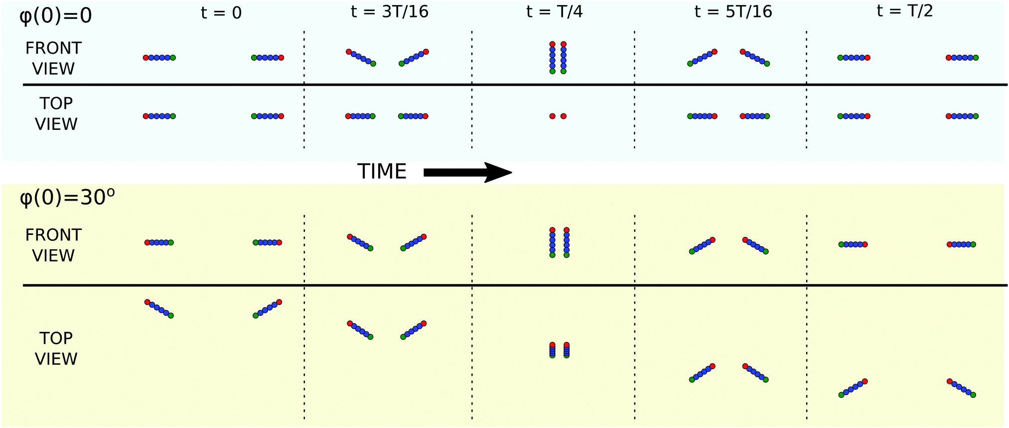 | ||
| Fig. 2 Snaphots from the periodic dynamics of a symmetric pair of rods. Top panel: Quasi-2D dynamics of rods (φ(0) = 0) showing tumbling motion reported before by Kim34 and Jung et al.41 Bottom panel: Periodic dynamics of rods not restricted to the vertical plane (here shown for φ(0) = π/6). Tumbling motion is combined with swinging along the ‘y’ horizontal axis, what is clearly visible in the top view of the system. | ||
Let us now consider another, very special initial configuration: the rods are horizontal and parallel to the symmetry plane (φ(0) = 90°). Based on time-reversal symmetry it is clear that the particles in such a configuration will neither approach each other, nor repel: their configuration remains constant, and their only motion is the rotation around the long rod axis combined with vertical settlement.
In the following paragraphs we describe the family of systems in which the particles are initially horizontal (θ(0) = 90°) and the value of φ(0) is in between the two limiting cases described above, 0 < φ(0) < 90°. In general the dynamics of a symmetric pair of rods (not restricted to a vertical plane) requires one to consider a system with five degrees of freedom: the distance of the rod center from the symmetry plane xcm(t) and two orientation angles, θ(t) and φ(t), defined in Fig. 1, together with vertical coordinate zcm and second horizontal coordinate ycm of the rod center-of-mass. However, the last two are the same for both rods, and therefore do not influence their relative motion and will not be analyzed in this work.
The periodic dynamics of rods out of plane is illustrated in the bottom (light yellow) panel of Fig. 2 (see also ESI,† Videos 1, 2 and the bottom panel of Fig. 13 in Appendix A). It is similar to the quasi-2D in-plane dynamics, but now particle rotation is coupled with swinging along the y axis in the laboratory reference frame.
The values of the θ and φ angles during the period are shown in Fig. 3A as closed curves, along which the system evolves counterclockwise (in this case, xcm(0) = 2). We may notice that although the value of the φ angle varies during the motion, it never reaches 0: if it did, the system would stay in the vertical plane forever.
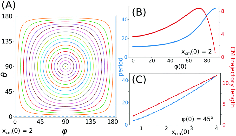 | ||
| Fig. 3 Properties of the rods’ periodic tumbling. (A) The rods’ orientation during the period, presented as the evolution of tilt angle θ and rotation angle φ. Different lines correspond to different initial values of φ, taken from range [0°, 90°] with step 5°. (B) and (C) Period of the motion and trajectory length (in the reference frame settling with the center of mass) as functions of the initial configuration parameters: rotation angle φ(0) (B) and initial distance xcm(0) (C). | ||
The dependence of the period on the initial configuration is presented in Fig. 3B and C. The shape of the blue curve in Fig. 3B is sigmoidal with a very small increase for φ(0) ≤ 30°. However, for larger values of φ(0), the initial rotation angle has a significant effect on the period. The shortest period is observed when the particles are in the vertical plane, and the longest for φ(0) → 90°: the difference between the extreme values is almost 5 fold. Larger φ(0) leads to longer periods because the particles do not approach each other as much as for smaller φ(0) and therefore, being on average more widely separated, their mutual interactions are weaker. It is noteworthy that the period of oscillations for growing φ(0) → 90° converges to a finite number which is larger than zero. In the limiting case, the two rods oriented along y do not change the positions of their centers, but they roll with a certain finite and non-vanishing frequency. In the same plot Fig. 3B but with a red color we show the length of the trajectory of the centers of rods, calculated in the reference frame settling with the particles. It may be observed that the trajectory length initially increases, reaches a maximum for about φ(0) ≈ 72° and sharply decreases for larger φ(0), hitting 0 for φ(0) = 90°. The total length of the trajectory (per period) measured in the laboratory reference frame is dominated by the settling of particles and therefore its shape is almost identical to the curve representing the period, shown in blue.
The influence of the initial distance between the rods on the period (Fig. 3C) is more straightforward: the period is longer for larger xcm(0) and the growth is very close to linear in terms of the trajectory length and slightly faster in terms of the period time. The relations in Fig. 3B and C are shown for xcm(0) = 2 and φ(0) = 45°, respectively.
In general, the initial symmetric configurations could have arbitrary values of θ. Not all of them lead to periodic motion. For example, it was shown by Kim34 that two rigid elongated particles in a symmetric configuration may either perform periodic motion, or have “single-encounter” dynamics and drift away from each other. For the rods, the horizontal symmetric initial configurations considered in this work (i.e. θ(0) = 90°) lead to periodic dynamics for almost all the considered values of φ(0), except for φ(0) = 90°, which is the stationary state. The closer ends of the rods sediment faster and therefore become lower than the other ones. In such a configuration, the lower ends are attracted to each other, but the upper ones are attracted even more, and as a result the rods rotate, and the angle between them decreases. At a certain time t‖, the end-to-end vectors become parallel to each other, with the corresponding angles θ(t‖) < π/2 and φ(t‖) = π/2. Let's denote the vertical positions of the rod centers at t‖ as y‖ and z‖. The occurrence of the parallel configuration guarantees that the motion is periodic. The justification is a simple modification of the arguments given in ref. 52. By superposition of the reflections in the horizontal and vertical planes, z = z‖ and y = y‖, and time reversal, it is straightforward to deduce that at time t = 2t‖, the rods will attain the horizontal configuration which is the mirror reflection y‖ − y → y‖ + y of the initial configuration.
The above reasoning can be applied to a wider class of identical rigid particles initially in horizontal symmetric configurations. In 3D motion it is sufficient that they have axial and fore–aft symmetries; in the quasi-2D dynamics (φ = 0) it is enough that apart from fore–aft symmetry the particles have a symmetry plane which coincides with the vertical plane of the motion (so that the system is truly quasi-2D). This explains the experimental findings of Jung et al.41 who found periodic oscillations of hemispheres and cubes sedimenting vertically.
The new family of 3D periodic solutions for rigid particles which has been presented in this section is interesting on its own. Moreover, our periodic solutions are important because they give a framework to understand the dynamics of deformable particles, and in particular elastic filaments.
4 Dynamics of elastic filaments
4.1 General picture
The dynamics of elastic filaments is rich. Four different modes, observed for filaments with different elasticity, are shown in Fig. 4 and in ESI,† Videos 3 and 4. If the flexibility of the filaments is very low, the particles perform periodic motions similar to rigid rods. The difference is that the amplitude of the oscillations gradually decreases and after a long time the filaments end up in a parallel and horizontal configuration where no oscillations occur. In Fig. 4A snapshots of the filament configuration illustrate damping of oscillations for B = 10 and φ(0) = 45°: positions marked as 1st, 3rd and 4th are shown for consecutive moments when the end-to-end vector is horizontal.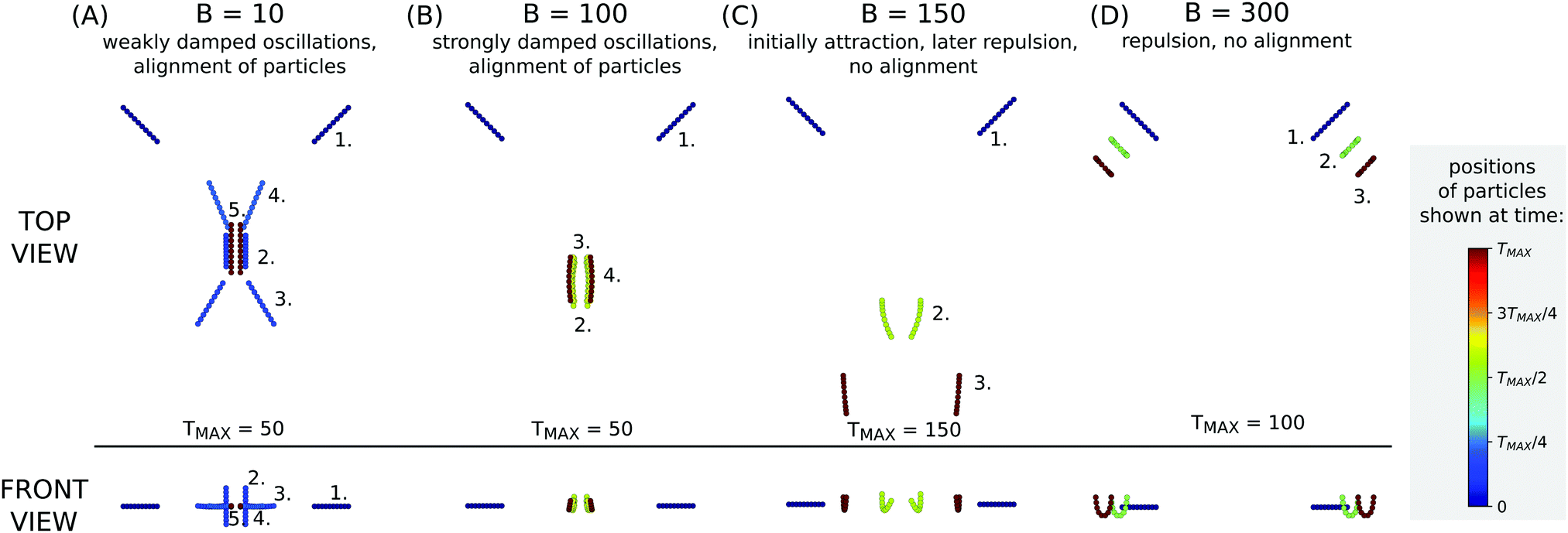 | ||
| Fig. 4 Different types of dynamics of elastic particles. The colors of the particles indicate the time when the snapshot was taken with respect to TMAX, different for each B. Low flexibility (B = 10): the particles perform tumbling motion, but the amplitude of the oscillations decreases. Finally the particles align in a horizontal configuration. The dynamics after alignment is discussed in the next section. Moderate flexibility (B = 100): for more flexible filaments the damping of the oscillations is faster, for B = 100 shown here it is almost instantaneous. Large flexibility (B = 150): even more flexible filaments first approach each other and later drift apart. Unlike for B = 100, the orientation angle φ does not reach π/2. Very large flexibility (B = 300): very elastic particles repel each other straight away, without approaching the attractive phase observed for smaller B = 150. Dynamics shown for xcm(0) = 2. | ||
Damping of the oscillatory motion is stronger for more elastic filaments. Fig. 4B illustrates that for B = 100 the filaments align almost instantaneously. For even more elastic filaments the particles do not oscillate and start to repel each other before reaching the parallel configuration. In Fig. 4C this kind of behavior is illustrated for B = 150 where the number 2 marks the position where the distance between the filaments is minimal. If the filaments are even more elastic, the filaments repel each other from the beginning of the simulation, as shown in Fig. 4D for B = 300.
In this paper we focus on the dynamics of weakly elastic filaments (small B), which are the most common in current applications. In this regime we observe a convergence of the filaments to an aligned, horizontal configuration, in which the orientation of the end-to-end vector is given by θ = 90° and φ = 90°. The convergence to the aligned configuration is shown in Fig. 5A. Oscillatory behavior of the system (compare with the rigid particles in Fig. 3A) is coupled with damping, which is faster for more elastic filaments.
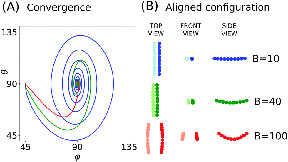 | ||
| Fig. 5 (A) Convergence to the aligned configuration shown in terms of orientation angles θ and φ. The orientation angles are plotted against each other for low flexibility (B = 10, blue line), moderate flexibility (B = 40, green) and high flexibility (B = 100, red). (B) Configuration of the filaments after alignment – when the orientation angles θ and φ remain constant. Deformation of filaments is very moderate, even for more flexible fibers of B = 100. For stiffer filaments with B = 10 the deformation is almost invisible. | ||
The damping of oscillations is relatively easy to explain. It is known that a single bent filament rotates to the horizontal configuration,20,23 where ‘horizontal’ is understood as the orientation of the end-to-end vector. Now consider the dynamics of two weakly flexible filaments, arbitrarily close to the limit of stiff rods. Since the filament is almost rigid, the dominant mode of dynamics is the periodic motion described in the first section of this work. Periodic oscillations, characteristic for stiff rods, are coupled with the effects of the filament flexibility: due to gravity they are weakly bent, which induces their slow rotation toward the horizontal configuration. The combination of these two effects results in a characteristic spiral form of the orientation plot (Fig. 5A).
The effect of alignment is strong even for weakly flexible filaments, which is the most common case encountered in experiments. Fig. 5B shows the configuration of the filaments after the oscillations have been damped and the filaments have aligned. We may observe that a value of elasticity parameter B = 10 corresponds to almost rigid filaments. In fact, even more rigid filaments converge to a parallel configuration, for example with B = 1, which corresponds to a filament which would bend§ only by 0.0015 of its length while sedimenting in a quiescent fluid (in the case of B = 10 the bending amplitude is equal to 0.015 of the filament length).
4.2 Decay of the oscillation amplitude
In order to define the amplitude of the oscillations, we choose shifted extrema of θ(t); more specifically, extrema of θ(t) − 90°, which is the angle between the horizontal plane and the orientation vector. Its value is equal to 0 in horizontal configurations and has local extrema in parallel ones. A selected example of θ(t) − 90° as a function of time is shown in Fig. 6A, with the extrema marked with dots in order to visualize points at which the oscillation amplitude is measured. | ||
| Fig. 6 Decay of the oscillation amplitude. (A) Angle θ(t) − 90° as a function of time for a selected example B = 10, φ(0) = 45° and xcm(0) = 3. Dots indicate local extrema. The inset shows time intervals between consecutive extrema of θ. (B) Exponential decay of the oscillation amplitude, the fitted relation is shown with a black line. In the inset the dependence of the amplitude ratio r is shown as a function of the filament elasticity. | ||
We observe that the decay of the oscillation amplitude is exponential with respect to number of oscillations (Fig. 6B). Therefore the amplitude of the n-th oscillation A(n) can be written as:
| A(n) = A0rn, | (8) |
If the amplitude is considered as a function of time, instead of the number of oscillations, the observed decay is not exponential (nor power-law). Also, the interval between consecutive (t) extrema is not conserved, as shown in the inset in Fig. 6A.
The speed of the exponential decay of the oscillation amplitude depends on the filament flexibility and is larger for more elastic particles (see also ESI,† Videos 3 and 5). The inset in Fig. 6B illustrates the dependence of the amplitude ratio r on the flexibility B. As expected, for very stiff particles r is close to the limit of 1, which characterizes undamped periodic motion. Damping becomes stronger for growing B and more flexible filaments may perform only a few oscillations before the amplitude of the oscillations decays to negligibly small values. For an initial configuration close to φ(0) = 0 or φ(0) = 90° the exponential fit is not so perfect as for the case of φ(0) shown in Fig. 6, however this type of dependence can be still observed, especially for small angles θ(t) − 90°.
4.3 Comparison to a single filament
In previous sections of this chapter it was shown that a symmetric pair of filaments converges to an aligned, horizontal configuration. Because it is known that also an isolated, single filament orients itself horizontally, it is interesting to study whether the presence of another filament promotes or hampers the filament reorientation. In other words, the question is whether two particles in a symmetric configuration converge to a horizontal configuration faster than the single one or slower. In order to investigate this problem, the dynamics of a single filament was evaluated for an initial configuration identical to the configuration of one from the pair of sedimenting filaments at chosen moments, when |θ − 90°| has local maxima. Representative results are presented in Fig. 7 where the values of θ − 90° in the system of the two particles are plotted with blue lines while the values of θ − 90° for a single filament are plotted with black, dashed lines. Each dashed line corresponds to an alternative dynamics in which the ‘left’ particle from the pair instantaneously ‘disappears’. For each simulation of the dynamics of the two particles a series of simulations of one filament were conducted, for different initial configurations. It is visible that in all cases the single filament converges toward θ = 90° faster than the pair of filaments. As it is shown in the figure, this result holds for different values of the elasticity. | ||
| Fig. 7 Convergence of the symmetric system of two particles toward the horizontal orientation (θ − 90° shown in blue), in comparison with the system of a single particle (θ − 90° shown with black dashed lines). Local extrema of θ − 90° are marked in orange, some of them were used to obtain the initial configurations for the single filament dynamics. Note the different time scales in different panels. All results shown for systems of two particles are obtained for initial configurations xcm(0) = 2 and φ(0) = 45°. | ||
The important conclusion from this study is that two flexible filaments, owing to the hydrodynamic interactions, orient themselves horizontally much slower than a single filament, if they are relatively stiff. In particular, for B = 1 shown in the top panel of Fig. 7, the two filaments need additional time to reorient to the parallel configuration because they oscillate, and therefore they bend slower than a single one. This result was obtained for a strictly symmetric configurations of two filaments, however in Section 6 it will be shown that the ‘aligning’ dynamics of filaments is robust to even large deviations from the symmetry and therefore the conclusion drawn here may be valid for a wider range of systems.
4.4 Dynamics after alignment
When the filaments reach the parallel, horizontal configuration, their relative motion usually does not stop. Depending on their flexibility the particles may attract each other, repel, or converge toward a stationary state. Signs of such migration are visible in Fig. 4A–C. In order to investigate this phenomenon more closely we performed simulations of filaments which start from aligned configurations (φ(0) = 90°, θ(0) = 90°) for different initial separation distances and different filament flexibility B.The results show that filaments of low and moderate flexibility (B ≤ 74) attract each other and eventually collide, and more elastic filaments (75 ≥ B ≤ 124) tend to stationary well separated configurations while even more elastic ones repel each other even at huge distances. These three regimes are illustrated in ESI,† Video_06. Considering the regimes of low and moderate B it is important to remark that the Rotne–Prager–Yamakawa approximation of hydrodynamic interactions, used in this work, is not an appropriate tool to model the dynamics of very close filaments, which tend to collide. More accurate methods, such as the multipole approximation with lubrication correction53 should be applied, which will be the topic of future studies. However, the results obtained allow us to conclude that moderately flexible filaments attract each other, without specifying whether the distance between them asymptotically decreases to 0 or they converge to a very close, yet separated configuration.
Moderately flexible filaments, approximately in a relatively narrow range of B ∈ [75, 124], converge to a stationary configuration, which is illustrated in Fig. 8A for selected values of B. Fig. 8B shows the distance between the centers of the filaments as a function of time, for two different initial configurations (xcm = 0.1 and xcm = 1.0). Convergence of both results is clear for each value of B. The separation of the particles at the stationary state is larger for more elastic filaments and increases rapidly for B > 124. For large B the stationary state may either exist at very large separations (e.g. larger than 100 for B = 125), or may not exist at all. It is worth noting that the drift of the filaments in the aligned configuration usually is very slow, which can be also observed in ESI,† Video_06.
 | ||
| Fig. 8 Stationary configurations of flexible filaments. (A) Stationary configurations with different values of B, drawn to scale. (B) Convergence towards a stationary configuration shown in terms of the distance between the centers of the filaments, for aligned initial configurations with different values of xcm(0): xcm(0) = 0.1 and xcm(0) = 1. | ||
5 Rigid filaments with curved shapes
The origin of the alignment phenomenon suggests that it may occur not only for elastic particles. The key factor of the process is self-reorientation of each particle, so that it tends to a horizontal configuration. An example of such particles is rigid fibres with curved shapes.26,27We analysed the family of rigid shapes derived from the equilibrium configurations of isolated elastic filaments of different elasticity. Therefore the family of rigid particle shapes is parameterized by B, where small B corresponds to more straight shapes and large B to more curved. In this way there is a direct correspondence between elastic filaments and rigid, curved particles, which will be explored in the following paragraphs.
The results show that rigid, curved particles behave in the same way as flexible ones: oscillations with decreasing amplitude are observed, after which the particles converge to the aligned, horizontal configuration. Rigid particles with shape parameterized by a given B perform almost the same motion as elastic ones with the corresponding value of the flexibility parameter. These phenomena can be observed both in the θ, φ phase space (Fig. 9A) and as the evolution in time (Fig. 9B). It is also illustrated in ESI,† Video_07.
 | ||
| Fig. 9 (A) Convergence toward an aligned configuration of rigid particle shapes corresponding to: B = 10 (blue), B = 40 (green) and B = 100 (red). For comparison, results for flexible filaments are drawn with dotted lines. (B) Comparison of the orientation angle θ(t) for rigid curved particles (blue line) and flexible particles with B = 10 (gray line). (C) Stationary configuration for different shapes of rigid particles (here ‘B’ denotes the shape of the particle, as explained in the main text). (D) Convergence of rigid curved particles of different shapes towards a stationary state. | ||
After the alignment, similarly to the flexible fibres, the curved particles can attract each other, repel, or converge toward a stationary distance. The last of these scenarios is illustrated in Fig. 9C and D. The stationary distance toward which the particles converge is very sensitive to the fibre shape. Additionally, the stationary distance of rigid particles parameterized by a given B is noticeably different than in the case of their flexible counterparts, even though the oscillatory phase of the dynamics is almost identical. This suggests that the stationary distance may differentiate pairs of particles based on very small differences of their properties.
6 Non-symmetric configurations of elastic particles
Generally, particles in slightly non-symmetric configurations behave in a very similar way to those in the symmetric systems. We introduced a perturbation of the initial configuration by modifying only the right filament (placed in the x > 0 half space). We kept it straight but altered its position with four different types of disturbances, illustrated in the top panel of Fig. 10: a modified ‘y’ coordinate (denoted as a Δy perturbation), a changed ‘z’ coordinate (Δz), changed θ(0) (Δθ) and finally changed φ(0) (Δφ). The translational perturbations, Δy and Δz, were tested up to 1/10 of the filament length while the rotational ones, Δθ and Δφ, up to 10°. | ||
| Fig. 10 Evolution of a non-symmetric pair of elastic filaments. In the top panel four types of initial perturbations are illustrated. Note that in the case of Δθ the rotation is around the horizontal axis perpendicular to the particle. In the middle panel the asymmetry of the system is shown for different types (see the legend) and different amplitudes of initial perturbations. For stiff particles (B = 1) the initial perturbations amplify, while for more flexible ones (B = 40) they attenuate. In the bottom panel trajectories of the beads are shown (top view) in the laboratory and in the moving reference frames for initial perturbation Δz = 0.02, for which the system converges to a symmetric, aligned configuration. The initial and final positions of the beads are marked in grey. | ||
For larger values of the elasto-gravitational number considered in this work, B ∈ [10, 100], the observed dynamics is robust to perturbations and the filaments converge to a symmetric, horizontal, aligned configuration. Only for very stiff particles does the system become unstable – initial non-symmetric perturbations amplify. In Fig. 10, middle panel, the asymmetry of the system is traced in time for very stiff (B = 1) and moderately flexible (B = 40) filaments. The asymmetry is measured as the root square deviation between the positions of the beads from the first particle and the reflected position of the beads from the second particle. The vertical reflection plane was chosen, at each moment separately, to minimize the expression: 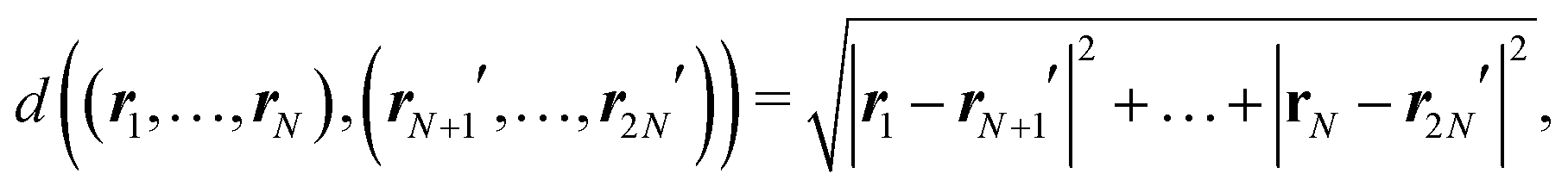 where ri′ denotes the reflection of the i-th bead position ri.¶ The results presented in Fig. 10 show that for very stiff fibres the initial perturbations amplify, while for more elastic particles the perturbations attenuate (the particles align), except a transient excitation when the particles are close to each other (in Fig. 10, a maximum is visible at t ≈ 15). Both types of behavior are new and important. Undoubtedly, the alignment behaviour is more interesting, because it occurs for a flexibility range which is commonly considered in studies concerning the dynamics of fibres, e.g. periodic motions of three fibres,32 and reveals an attractor of the two-filament dynamics. Nevertheless, the unstable behaviour of stiffer particles is also a meaningful result, indicating the possibility of transient chaos in the system of two settling particles.54
The bottom panel of Fig. 10 presents bead trajectories (top view) for a selected example of a system in which alignment occurs (Δz = 0.02, see also ESI,† Video_08). It can be observed that the alignment is preceded by an intricate, oscillatory phase of the dynamics. In the moving reference frame, the alignment of particles is clearly visible and it becomes evident that rotation and drift of the pair, observed in the laboratory reference frame, is caused by only minor asymmetry of the system. The moving reference frame was chosen in such a way that the center of mass of the system does not move horizontally, and the new ‘x’ axis is parallel to the minimal asymmetry plane. Alignment of filaments, observed for a wide range of asymmetric configurations, suggests that the parallel configuration of filaments is an important attracting state for the dynamics (not forgetting that the aligned configuration is not always static – see Section 4.4 – as the distance between the aligned filaments may change).
Unlike for more elastic filaments, stiffer particles with B < 10 rarely align. Different types of the observed behaviors are shown in Fig. 11 and Videos 9–12. The dynamics becomes very sensitive to the perturbations of the initial configuration and the filaments usually collide (Fig. 11B and Video_10). Two new types of long-lasting configurations have been observed, which are illustrated in Fig. 11C (Video_11) and D (Video_12). In the former, the end-to-end vectors of the filaments are parallel, but one particle is higher than the other and the fibres are shifted in the horizontal direction, perpendicular to the fibre orientation. Such an arrangement leads to horizontal movement of the pair of particles. It was shown before31,32 that in similar configurations the upper particle settles faster and finally catches up with the lower one, yet this process is very slow, especially for stiffer particles. In the second type of configuration (Fig. 11D) the centres of the particles are one above the other, but the fibres are not parallel. Such a configuration was studied by Saggiorato et al.,32 who observed that it leads to helical movement of the filaments, which is in agreement with our results. In the long term the upper particle would catch up with the lower one, and at the same time the orientations of the two fibres become more and more similar.
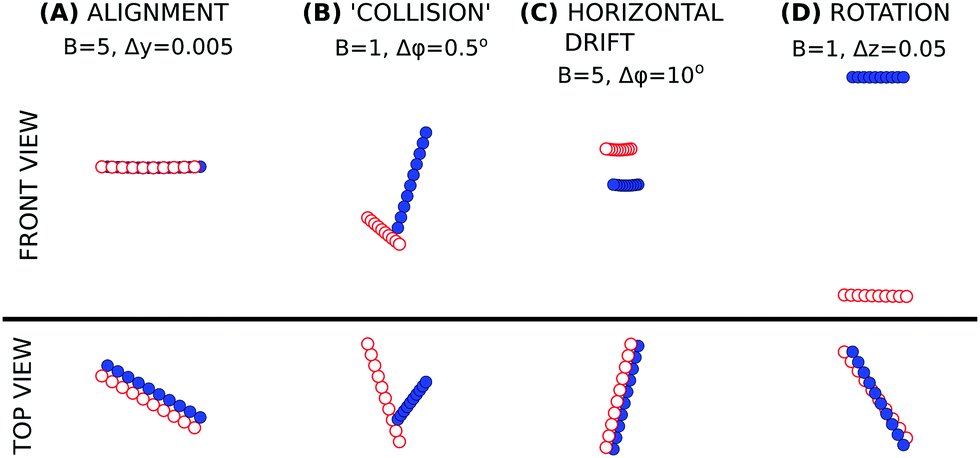 | ||
| Fig. 11 Observed behaviors of stiffer fibres: (A) alignment (rare); (B) collision (common); (C) horizontal drift (rare); and (D) rotation (rare). The dynamics leading to the configurations illustrated above is presented in ESI,† Videos 9–12. | ||
The behaviour of the non-symmetric pairs of filaments is summarized in Fig. 12. It shows a wide range of the parameter B, which corresponds to fibres of different flexibility, or to a variable strength of the external field – which can be found e.g. under gravity, in a centrifuge or for electrically-driven motion of charged particles. The stiffest filaments (B < 10) often collide during the simulations, and the contact between them is established at ‘random’ points. More flexible ones (10 ≤ B ≤ 75) first converge to a parallel configuration, and on a longer time scale approach each other in the parallel configuration. The contact is established at the ends of the fibres, yet the particles are close to each other all along their length. Even more flexible fibres (75 < B < 124) also converge to a parallel configuration, but unlike in the previous case, they avoid contact. Very flexible filaments (B > 150) avoid contact without forming stable pairs. Independently of the flexibility of the filaments, if the perturbation is large in some cases ‘simple’ collisions may be observed, which are typical for stiff particles (B < 10). From the description given above we can conclude that by varying the strength of the external field, the flexibility of the filaments or the fluid density, one may control the way in which two particles interact in the Stokes flow and how far they are from each other.
 | ||
| Fig. 12 Influence of the external field (e.g. gravity) magnitude on the type of the dynamics in a non symmetrical system. Typical configurations are shown for B ∈ {1, 40, 100}. | ||
7 Discussion and conclusions
In this article, we present new periodic orbits of rigid rods not restricted to a vertical plane. We also explain why symmetric pairs of rods initially in a horizontal configuration must perform periodic motions. The basic features of such dynamics, e.g. the dependence of the period on the initial configuration, have been examined.The periodic dynamics of rigid particles is key to explain the dynamics of weakly bending filaments, which are of particular interest because most physical systems studied experimentally fall into this regime of small flexibility B. Weakly bending filaments, initially in a symmetric horizontal configuration, later perform oscillations similar to rigid rods, but with time, the amplitude of the oscillations diminishes and the particles converge to a parallel, horizontal configuration. We provide an explanation of this behavior and show that the decay of the oscillation amplitude is roughly exponential with respect to the number of oscillations (but not with respect to time). We also show that damping of oscillations is faster for more flexible filaments, and for moderate flexibility, B ≈ 100, it is almost instantaneous.
After alignment, stiffer filaments approach each other and, under the RPY approximation, eventually collide. Moderately flexible filaments converge to a well-separated configuration, and even more flexible ones drift apart.
The mechanism of the alignment of flexible fibres was shown to depend solely on their bent shape. This observation allowed us to extend the applicability of the results to rigid, curved particles. In the studied system, rigid particles behave almost identically to their flexible counterparts, given that the fixed, curved shape of the former is similar to that adopted under gravity by the latter ones. The key factors of particle alignment are their elongated shape (which entails their initial drift toward each other and the movement along the y axis) combined with the ability of each curved particle to orient itself perpendicularly to gravity or another external force driving the system. As a result, the findings obtained here for flexible filaments may be applicable to a wide class of elongated particles which self-orient while sedimenting, e.g. banana-shaped rigid particles55 or crescent-shaped sickle red blood cells in sickle cell disease.56
Additionally, we briefly discussed the dynamics of more flexible filaments, B ≥ 150 for N = 10. In this case the filaments do not align, but drift apart in a non-parallel configuration. If the filaments are not too flexible, e.g. B ≈ 150 for φ(0) = π/4, the particles first approach each other and later repel. In the case of even more flexible filaments, e.g. B ≥ 200, the particles drift away from each other immediately, without an attracting phase.
During the studies of the dynamics of flexible filaments, in addition to the presented results for N = 10, we also investigated the dynamics of shorter and longer filaments, consisting of N ∈ {6, 13, 20, 30} beads. Qualitatively the dynamics are the same as for the shorter fibers and only minor, quantitative changes are observed. Filaments consisting of up to N = 30 beads may perform all modes of symmetric dynamics presented in Fig. 4. In particular, fibres converge to the aligned configuration for a very similar range of B. Also in the parallel configuration particles behave in the same way as shorter filaments: flexibility-dependent attraction, repulsion, or convergence to a steady distance is observed. The aspect ratio of the filaments (number of beads) influences slightly the limiting value of B between different modes of the dynamics, as well as the B-specific equilibrium distance for the parallel filaments (see Fig. 8). In particular, the upper limit of φ(0) for which collisions of the filaments are observed (instead of alignment) is larger for longer fibres. Due to their larger mobility in the elongated direction, thinner particles collide more easily than thicker ones. Overall, however, the main effect of different filament length (or aspect ratio) is included in the dimensionless parameter B = 4GL02/πEYa4. The quantitative effects, mentioned above, are secondary. The dynamics of filaments with the same values of B are similar to each other for a wide range of aspect ratios.
The range of the considered values of B chosen in this article often corresponds to elongated flexible filaments which can be found in nature, and also those which were studied theoretically in the literature, as discussed in ref. 45.
One of the fields in which our results may apply is the dynamics of chain-forming diatoms.13,14,16 These non-motile phytoplankton species have an important role in marine food webs.13 The diatom chains have a diameter of about 20–50 μm and a density of 1.1 kg dm−3. Their bending stiffness (corresponding to the parameter A) is estimated as 1.3 × 10⁻¹⁷ Nm2 for Guinardia delicatula up to 1.7 × 10⁻¹³ for Lithodesmium undulatum.14 Some diatom species can be even more flexible.14 In terms of the elasticity-to-bending parameter B, a hypothetical diatom of diameter d = 20 μm, density ρ = 1.125 kg dm−3, chain bending stiffness A = 1.3 × 10⁻¹⁷ and length 750–2000 μm corresponds to B ∈ [10, 200], investigated in this paper.
In conclusion, in this paper we provide a description of the dynamics of two sedimenting particles for a wide range of their elastic properties: from very stiff to very flexible. The most attention is devoted to relatively stiff particles, due to their importance in applications. Additionally, a physical explanation is given for the most important features of the observed dynamics: periodic motions of rigid particles and convergence to an aligned configuration by elastic filaments.
This study reveals a few interesting problems for future work. It is worthwhile to examine the dynamics of filaments after alignment with the use of a more accurate approximation of hydrodynamic interactions between the beads, such as the multipole expansion of the Stokes equations corrected for lubrication, implemented in the numerical code Hydromultipole.53 In this way, it would be possible to avoid spurious collisions and determine the dynamics of filaments with some of the beads coming very close to each other. Moreover, it would allow one to reveal whether attracting, stationary, non-touching aligned configurations exist for relatively stiff filaments. For more flexible filaments it is important to study the dynamics after alignment, in order to know the long-term dynamics of the filaments. The transition between the alignment regime (smaller B) and non-alignment/repulsion regime (larger B) also remains to be analyzed. Moreover, it is worthwhile to study if there exist different stationary or periodic solutions for two sedimenting flexible filaments, and analyze their stability properties. Comparison with experiments would be also important. Moreover, it is interesting to investigate how the dynamics and rheology of suspensions of flexible fibers57–59 is affected by pairwise hydrodynamic interactions between elastic filaments. For example, in sedimenting suspensions, flexibility causes elongated particles to preferentially align in directions perpendicular to gravity.58 As shown in this paper, a pair of flexible filaments shares this commonality. Finally, it would be worthwhile to study hydrodynamic interactions of pairs of sedimenting elastic loops.46,60
Conflicts of interest
There are no conflicts of interest to declare.Appendix A: filament trajectories
In Fig. 13 and 14, we present trajectories of two rigid and two elastic symmetric filaments, respectively. We plot the trajectories of each bead in the laboratory frame of reference. The examples shown are representative also for other values of the parameters. The trajectories in Fig. 13 and 14 correspond to the snapshots presented in Fig. 2 and 4 in the main text.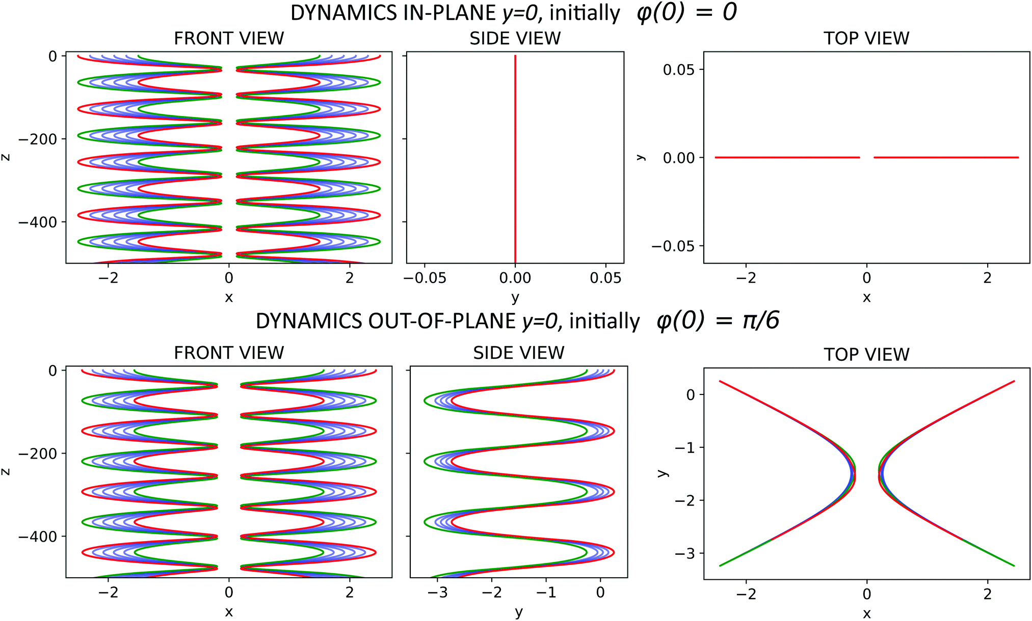 | ||
| Fig. 13 Dynamics of rigid rods made of N = 6 beads in the laboratory frame of reference. Trajectories of bead centers with labels 1, 6 and 2, 3, 4, 5 are marked with red, green and blue, respectively. Initially xcm(0) = 2. Top row: quasi-2D vertical sedimentation for φ(0) = 0. Bottom row: 3D motion for φ(0) = π/6. | ||
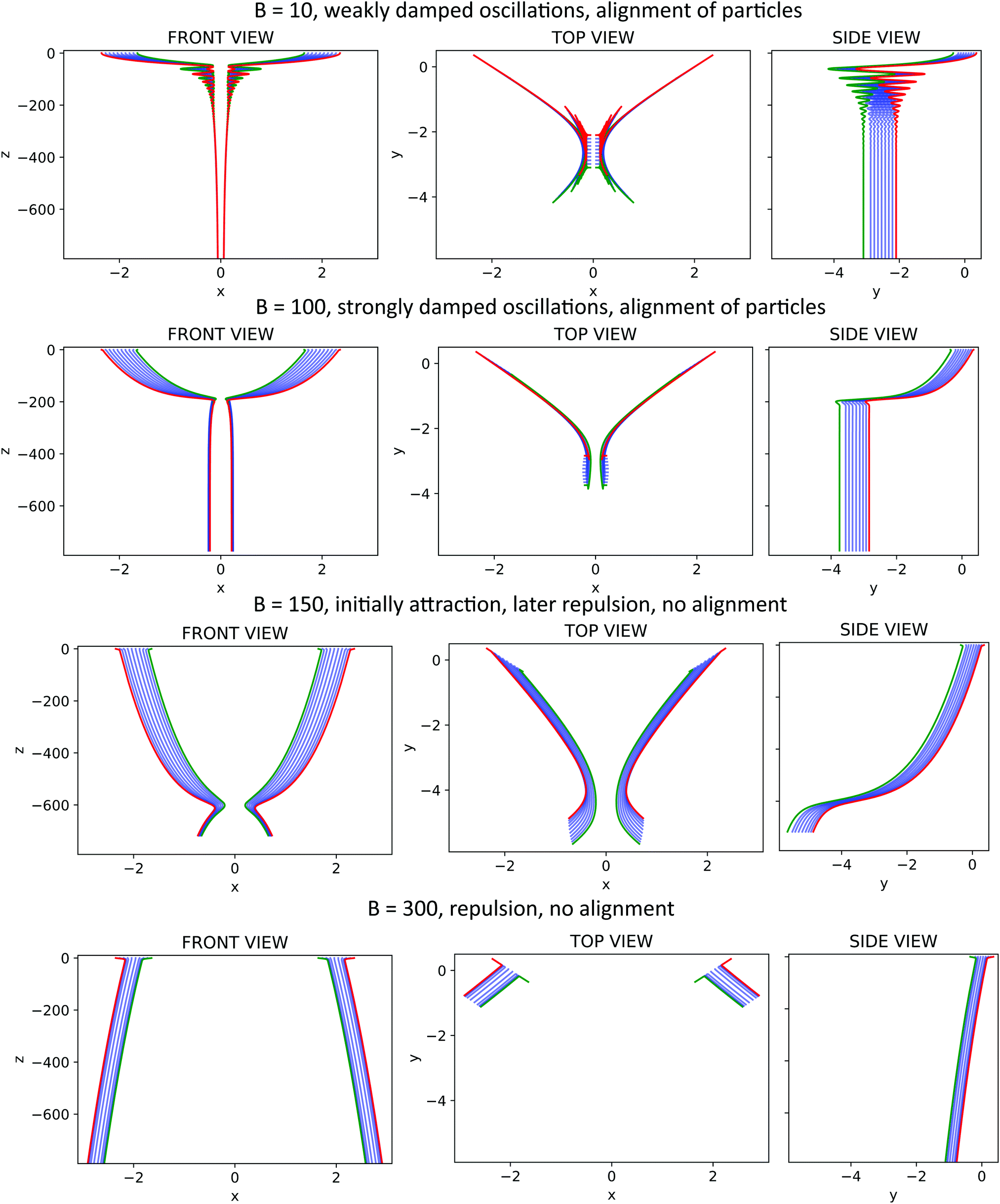 | ||
| Fig. 14 Dynamics of two flexible filaments in the laboratory frame of reference, for the same parameters as in Fig. 4: N = 10, xcm(0) = 2, φ(0) = π/4 and the elasto-gravitational number B as indicated. Trajectories of all the beads are shown: green and red – first and last bead of each filament, blue – other beads. | ||
Appendix B: list of supplementary videos
Video_01 Periodic motions of rigid, straight particles consisting of 6 beads. φ(0) = 30°.Video_02 Periodic motions of rigid, straight particles consisting of 10 beads. φ(0) = 45°.
Video_03 Dynamics of moderately elastic fibers, where the particles converge to the aligned configurations. N = 10, φ(0) = 45°.
Video_04 Dynamics of very elastic fibers, which converge to a specific distance (B = 100) or repel each other (B = 150, B = 300). N = 10, φ(0) = 45°.
Video_05 Influence of the fiber elasticity on the oscillation decay. Stronger damping is observed for more flexible particles. N = 10, φ(0) = 45°.
Video_06 Dynamics of parallel fibers (front view). Depending on their elasticity, the particles attract each other (most stiff), repel (most flexible) or converge to a specific distance (intermediate elasticity). N = 10, φ(0) = 90°.
Video_07 Dynamics of flexible filaments (B = 40) and rigid, curved particles with shape corresponding to the same elasticity. ‘Correspondence’ is defined in the main text. N = 10, φ(0) = 45°.
Video_08 Dynamics of a non-symmetric system which converges to the aligned configuration. N = 10, B = 10, φ(0) = 45°, Δz = 0.02.
Video_09 Dynamics of a non-symmetric system which converges to the aligned configuration. N = 10, B = 5, φ(0) = 45°, Δy = 0.005.
Video_10 Dynamics of a non-symmetric system where finally the particles collide. N = 10, B = 1, φ(0) = 45°, Δφ = 0.5°.
Video_11 Dynamics of a non-symmetric system where in the final stage the particles drift horizontally while settling down. N = 10, B = 5, Δφ = 0.5°, Δφ = 10°.
Video_12 Dynamics of a non-symmetric system where in the final stage the particles rotate around the vertical axis while settling down. N = 10, B = 5, φ(0) = 45°, Δz = 0.1.
Acknowledgements
This work was supported in part by Narodowe Centrum Nauki under grant no. 2014/15/B/ST8/04359.References
- H. C. Berg and D. A. Brown, Nature, 1972, 239, 500–504 CrossRef CAS PubMed.
- H. C. Berg and R. A. Anderson, Nature, 1973, 245, 380 CrossRef CAS PubMed.
- V. Kantsler and R. E. Goldstein, Phys. Rev. Lett., 2012, 108, 038103 CrossRef PubMed.
- M. Harasim, B. Wunderlich, O. Peleg, M. Kröger and A. R. Bausch, Phys. Rev. Lett., 2013, 110, 108302 CrossRef PubMed.
- Y. Liu, B. Chakrabarti, D. Saintillan, A. Lindner and O. du Roure, Proc. Natl. Acad. Sci. U. S. A., 2018, 115, 9438–9443 CrossRef CAS PubMed.
- E. Reed and H. Wallace, Nature, 1965, 206, 210 CrossRef.
- A. Bilbao, E. Wajnryb, S. A. Vanapalli and J. Blawzdziewicz, Phys. Fluids, 2013, 25, 081902 CrossRef.
- J. K. Nunes, K. Sadlej, J. I. Tam and H. A. Stone, Lab Chip, 2012, 12, 2301–2304 RSC.
- E. Wandersman, N. Quennouz, M. Fermigier, A. Lindner and O. Du Roure, Soft Matter, 2010, 6, 5715–5719 RSC.
- S. Pawłowska, P. Nakielski, F. Pierini, I. K. Piechocka, K. Zembrzycki and T. A. Kowalewski, PLoS One, 2017, 12, e0187815 CrossRef PubMed.
- A. Perazzo, J. K. Nunes, S. Guido and H. A. Stone, Proc. Natl. Acad. Sci. U. S. A., 2017, 114, E8557–E8564 CrossRef CAS PubMed.
- W. Lei, D. Portehault, D. Liu, S. Qin and Y. Chen, Nat. Commun., 2013, 4, 1777 CrossRef PubMed.
- E. V. Armbrust, Nature, 2009, 459, 185 CrossRef CAS PubMed.
- A. M. Young, L. Karp-Boss, P. Jumars and E. Landis, Limnol. Oceanogr., 2012, 57, 1789–1801 CrossRef.
- M. M. Musielak, L. Karp-Boss, P. A. Jumars and L. J. Fauci, J. Fluid Mech., 2009, 638, 401–421 CrossRef CAS.
- H. Nguyen and L. Fauci, J. R. Soc., Interface, 2014, 11, 20140314 CrossRef PubMed.
- J. LaGrone, R. Cortez, W. Yan and L. Fauci, J. Non-Newtonian Fluid Mech., 2019, 269, 73–81 CrossRef CAS.
- A. Lindner and M. Shelley, Fluid-Structure Interactions in Low-Reynolds-Number Flows, Royal Society of Chemistry, 2015, pp. 168–192 Search PubMed.
- O. du Roure, A. Lindner, E. N. Nazockdast and M. J. Shelley, Annu. Rev. Fluid Mech., 2019, 51, 539–572 CrossRef.
- X. Xu and A. Nadim, Phys. Fluids, 1994, 6, 2889–2893 CrossRef.
- X. Schlagberger and R. Netz, Europhys. Lett., 2005, 70, 129 CrossRef CAS.
- M. Manghi, X. Schlagberger, Y.-W. Kim and R. R. Netz, Soft Matter, 2006, 2, 653–668 RSC.
- M. Cosentino Lagomarsino, I. Pagonabarraga and C. Lowe, Phys. Rev. Lett., 2005, 94, 148104 CrossRef CAS PubMed.
- L. Li, H. Manikantan, D. Saintillan and S. E. Spagnolie, J. Fluid Mech., 2013, 735, 705–736 CrossRef.
- B. Marchetti, V. Raspa, A. Lindner, O. du Roure, L. Bergougnoux, É. Guazzelli and C. Duprat, Phys. Rev. Fluids, 2018, 3, 104102 CrossRef.
- M. L. Ekiel-Jeżewska and E. Wajnryb, J. Phys.: Condens. Matter, 2009, 21, 204102 CrossRef PubMed.
- E. Tozzi, C. T. Scott, D. Vahey and D. Klingenberg, Phys. Fluids, 2011, 23, 033301 CrossRef.
- B. Moths and T. Witten, Phys. Rev. Lett., 2013, 110, 028301 CrossRef PubMed.
- T. Goldfriend, H. Diamant and T. A. Witten, Phys. Fluids, 2015, 27, 123303 CrossRef.
- T. Goldfriend, H. Diamant and T. A. Witten, Phys. Rev. E, 2016, 93, 042609 CrossRef PubMed.
- I. Llopis, I. Pagonabarraga, M. Cosentino Lagomarsino and C. P. Lowe, Phys. Rev. E: Stat., Nonlinear, Soft Matter Phys., 2007, 76, 061901 CrossRef CAS PubMed.
- G. Saggiorato, J. Elgeti, R. G. Winkler and G. Gompper, Soft Matter, 2015, 11, 7337–7344 RSC.
- S. Wakiya, J. Phys. Soc. Jpn., 1965, 20, 1502–1514 CrossRef CAS.
- S. Kim, Int. J. Multiphase Flow, 1985, 11, 699–712 CrossRef CAS.
- S. Kim, Int. J. Multiphase Flow, 1986, 12, 469–491 CrossRef CAS.
- S. Kim and S. J. Karrila, Microhydrodynamics: principles and selected applications, Courier Corporation, 2013 Search PubMed.
- R. Kutteh, Phys. Rev. E: Stat., Nonlinear, Soft Matter Phys., 2004, 69, 011406 CrossRef PubMed.
- R. Kutteh, J. Chem. Phys., 2010, 132, 174107 CrossRef PubMed.
- D. Bartuschat, E. Fischermeier, K. Gustavsson and U. Rüde, Comput. Fluids, 2016, 127, 17–35 CrossRef.
- R. Chajwa, N. Menon and S. Ramaswamy, Phys. Rev. Lett., 2019, 122, 224501 CrossRef CAS PubMed.
- S. Jung, S. Spagnolie, K. Parikh, M. Shelley and A.-K. Tornberg, Phys. Rev. E: Stat., Nonlinear, Soft Matter Phys., 2006, 74, 035302 CrossRef PubMed.
- K. Gustavsson and A.-K. Tornberg, Phys. Fluids, 2009, 21, 123301 CrossRef.
- J. Rotne and S. Prager, J. Chem. Phys., 1969, 50, 4831–4837 CrossRef CAS.
- H. Yamakawa, J. Chem. Phys., 1970, 53, 436–443 CrossRef CAS.
- M. Bukowicki and M. Ekiel-Jeżewska, Soft Matter, 2018, 14, 5786 RSC.
- M. Gruziel, K. Thyagarajan, G. Dietler, A. Stasiak, M. L. Ekiel-Jeżewska and P. Szymczak, Phys. Rev. Lett., 2018, 121, 127801 CrossRef CAS PubMed.
- E. Gauger and H. Stark, Phys. Rev. E: Stat., Nonlinear, Soft Matter Phys., 2006, 74, 021907 CrossRef PubMed.
- L. Hocking, J. Fluid Mech., 1964, 20, 129–139 CrossRef.
- M. Bukowicki, M. Gruca and M. L. Ekiel-Jeżewska, J. Fluid Mech., 2015, 767, 95–108 CrossRef CAS.
- M. L. Ekiel-Jeżewska, Phys. Rev. E: Stat., Nonlinear, Soft Matter Phys., 2014, 90, 043007 CrossRef PubMed.
- M. Gruca, M. Bukowicki and M. L. Ekiel-Jeżewska, Phys. Rev. E: Stat., Nonlinear, Soft Matter Phys., 2015, 92, 023026 CrossRef PubMed.
- R. E. Caflisch, C. Lim, J. H. Luke and A. S. Sangani, Phys. Fluids, 1988, 31, 3175–3179 CrossRef.
- B. Cichocki, M. Ekiel-Jeżewska and E. Wajnryb, J. Chem. Phys., 1999, 111, 3265–3273 CrossRef CAS.
- I. M. Jánosi, T. Tél, D. E. Wolf and J. A. Gallas, Phys. Rev. E: Stat. Phys., Plasmas, Fluids, Relat. Interdiscip. Top., 1997, 56, 2858 CrossRef.
- I. R. Thorp and J. R. Lister, J. Fluid Mech., 2019, 872, 532–559 CrossRef CAS.
- X. Zhang, W. A. Lam and M. D. Graham, Phys. Rev. Fluids, 2019, 4, 043103 CrossRef.
- M. Keshtkar, M. Heuzey and P. Carreau, J. Rheol., 2009, 53, 631–650 CrossRef CAS.
- H. Manikantan, L. Li, S. E. Spagnolie and D. Saintillan, J. Fluid Mech., 2014, 756, 935–964 CrossRef CAS.
- E. Nazockdast, A. Rahimian, D. Zorin and M. Shelley, J. Comput. Phys., 2017, 329, 173–209 CrossRef CAS.
- M. Gruziel-Słomka, P. Kondratiuk, P. Szymczak and M. L. Ekiel-Jeżewska, Soft Matter, 2019, 15, 7262–7274 RSC.
Footnotes |
| † Electronic supplementary information (ESI) available: Movies. See DOI: 10.1039/c9sm01373c |
| ‡ Such a system may be considered as a single filament near a free surface located at the symmetry plane.45 |
| § The bending amplitude is defined as maxi(zi) − mini(zi) where zi are the vertical coordinates of the bead centres. |
¶ Also the reverse order of beads in the reflected particle was considered:  |
| This journal is © The Royal Society of Chemistry 2019 |