
 Open Access Article
 This Open Access Article is licensed under a Creative Commons Attribution-Non Commercial 3.0 Unported Licence
Bond orders of the diatomic molecules†
Taoyi Chen and
Thomas A. Manz*
and
Thomas A. Manz*
Department of Chemical & Materials Engineering, New Mexico State University, Las Cruces, NM 88001, USA. E-mail: tmanz@nmsu.edu
First published on 31st May 2019
Abstract
Bond order quantifies the number of electrons dressed-exchanged between two atoms in a material and is important for understanding many chemical properties. Diatomic molecules are the smallest molecules possessing chemical bonds and play key roles in atmospheric chemistry, biochemistry, lab chemistry, and chemical manufacturing. Here we quantum-mechanically calculate bond orders for 288 diatomic molecules and ions. For homodiatomics, we show bond orders correlate to bond energies for elements within the same chemical group. We quantify and discuss how semicore electrons weaken bond orders for elements having diffuse semicore electrons. Lots of chemistry is effected by this. We introduce a first-principles method to represent orbital-independent bond order as a sum of orbital-dependent bond order components. This bond order component analysis (BOCA) applies to any spin-orbitals that are unitary transformations of the natural spin-orbitals, with or without periodic boundary conditions, and to non-magnetic and (collinear or non-collinear) magnetic materials. We use this BOCA to study all period 2 homodiatomics plus Mo2, Cr2, ClO, ClO−, and Mo2(acetate)4. Using Manz's bond order equation with DDEC6 partitioning, the Mo–Mo bond order was 4.12 in Mo2 and 1.46 in Mo2(acetate)4 with a sum of bond orders for each Mo atom of ∼4. Our study informs both chemistry research and education. As a learning aid, we introduce an analogy between bond orders in materials and message transmission in computer networks. We also introduce the first working quantitative heuristic model for all period 2 homodiatomic bond orders. This heuristic model incorporates s–p mixing to give heuristic bond orders of ¾ (Be2), 1¾ (B2), 2¾ (C2), and whole number bond orders for the remaining period 2 homodiatomics.
1 Introduction
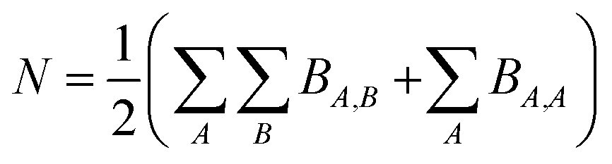
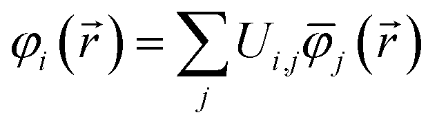
Because chemical bonds bind atoms to each other to form most chemicals and materials, a fundamental description of chemical bonds is essential to all chemical sciences. Although many chemical bonds contain electron pairs,1 other chemical bonds (e.g., [H2]+) do not contain any electron pairs. Common chemical bond descriptors include the chemical element identities, the bond length, the bond order (BO), the vibrational force constant for stretching the bond, and various bond energy descriptors.Although the general concept of BO originated more than a century ago (e.g., Lewis structures1), a comprehensive definition was proposed only as recently as 2017.2 According to this modern definition, the bond order BA,B between atoms A and B in a material is the quantity of electrons dressed-exchanged between them. Dressed-exchange is defined through the following equations related to the quantum mechanical exchange arising because electrons are fermions.2 First, the total number of electrons N in a material's unit cell can be partitioned between atom pairs:
 | (1) |
| BA,B = CEA,B + ΛA,B | (2) |
| 0 ≤ ΛA,B = χcoord_numA,BχpairwiseA,BχconstraintA,B ≤ CEA,B | (3) |
Manz's method is computationally efficient, derives from first-principles, applies to many bonding types and diverse materials, yields consistently accurate results across different quantum chemistry methods (e.g., CAS-SCF, CCSD, SAC-CI, DFT, etc.) and different SZ values of a spin multiplet, works well for non-equilibrium structures (e.g., stretched and compressed bonds, transition states), works with or without periodic boundary conditions, works with any basis set type (e.g., Gaussian, plane-wave, etc.) with low basis set sensitivity, and applies to non-magnetic systems as well as collinear and non-collinear magnetism.2 As shown in Table S1 of ESI† and prior literature,2 the DDEC6 BO is much more consistent across different quantum chemistry methods than the Mayer bond index.3
Manz's bond order is also more chemically consistent than the occupancy bond index (OBI). OBI = (sum of bonding orbital occupancies − sum of anti-bonding orbital occupancies)/2. As discussed in ref. 2, the OBI has two fundamental limitations:
(1) Different quantum chemistry methods (even if they are exact) can yield substantially different first-order density matrices and hence different NSOs and different OBI values. For example, DFT functionals yield idempotent first-order density matrices at absolute zero temperature, while correlated wavefunction methods (e.g., coupled-cluster, configuration interaction, etc.) yield first-order density matrices that are not necessarily idempotent. The NSO occupancies from DFT (at absolute zero temperature) are either 0 or 1, but can be anywhere over the interval [0,1] for correlated N-representable wavefunctions.4
(2) The OBI is unreliable for stretched bonds. As a bond is systematically stretched beyond its equilibrium value, the bonding or anti-bonding quality of individual NSOs or localized molecular orbitals may change abruptly even if the energy changes smoothly. This can cause the OBI value to change abruptly, even if the Manz BO changes smoothly. (See Fig. 1 of ref. 2 for a plot demonstrating this behavior for the natural localized molecular orbitals.)
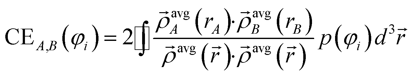
Manz's bond order equation requires the spherically averaged atom-in-material electron density ({ρavgA(rA)}) and spherically averaged atom-in-material spin magnetization density vector 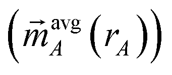 as inputs.2 These inputs must be assigned using a stockholder partitioning method. As in the prior study,2 we used this bond order equation with DDEC6 partitioning. DDEC6 partitioning gave good results across diverse material types.2,5–7 In this article, the term ‘DDEC6 bond order’ refers to the bond order computing using Manz's equation with DDEC6 partitioning, while the term ‘Manz bond order’ refers to bond order computed with this equation using any partitioning method.
There are no prior systematic studies of quantum-mechanically (QM) computed BOs across large numbers of diatomics. Two old, inaccurate (e.g., BOs of 1.55 for H2, 0.953 for P2, and 1.81 for HF), quasi-classical studies by Politzer estimated BOs for 21 homodiatomics and 54 heterodiatomics.8,9 Recently, Manz's study included accurate BOs computed via eqn (2) for 26 diatomics.2 Many studies (e.g., ref. 10–14 and others) calculated BOs for fewer diatomics. Here, we compute BOs for 288 diatomics to reveal systematic trends across the periodic table.
What is and is not yet known about BOs of diatomic molecules? There is widespread agreement on BOs for some diatomic molecules (e.g., BO = ∼1 for H2 and ∼3 for N2) but others (especially C2, but also Be2 and B2) were topics of substantial debate.15–18 S–p mixing was proposed as a semi-quantitative textbook argument for BOs of 0–1 for Be2, 1–2 for B2, and 2–3 for C2.15 Many computational studies of the C2 molecule argued its BO was (a) between 2 and 316,19–22 or (b) around 4.23–27 The C–C bond length in C2 (1.242 Å) is intermediate between ethylene (1.329 Å, heuristic BO = 2) and acetylene (1.203 Å, heuristic BO = 3).28 Since log(BO) is approximately linearly correlated to bond length,2,29 the interpolated C2 BO is log(BO) = log(2) + ((1.329 − 1.242)/(1.329 − 1.203))log(3/2) yielding BO = 2.65. Generalized valence bond (GVB) studies of C2 revealed four17,23,25 or three20 electron pairs with favorable energetic couplings. GVB studies of B2 revealed one strong plus one weak σ-bond components and two half-filled π-bond components.30
2 Results and discussion
2.1 Periodic trends of bond orders
First, we summarize the computed DDEC6 BOs: (a) Table 1 (65 homodiatomics) with additional information for these molecules listed in Table S2 of ESI,† (b) Table S3 of ESI† (217 heterodiatomics), (c) Table 2 (6 ions), and (d) Table S1 of ESI† (molecules and ions isoelectronic to C2). All of these tables list each molecule's spin multiplicity. Tables S2 and S3† compare calculated to experimental (where available) bond lengths and list the CRC handbook dissociation energies .28 Tables 2 and S3† also list net atomic charges (NACs) for the heterodiatomics. To the best of our knowledge, this is the largest collection of diatomics for which computed BOs have been reported. We computed the electron and spin density distributions using the coupled-cluster or configuration interaction methods CCSD, SAC-CI, or CAS-SCF selected to give reasonable agreement between calculated and experimental (where available) equilibrium bond lengths as summarized in Fig. 8.
| Spin mult. | Bond order | Spin mult. | Bond order | Spin mult. | Bond order | Spin mult. | Bond order | ||||
|---|---|---|---|---|---|---|---|---|---|---|---|
| H2 | 1 | 0.938 | Ar2 | 1 | 0.027 | Br2 | 1 | 1.264 | Xe2 | 1 | 0.048 |
| He2 | 1 | 0.004 | K2 | 1 | 0.705 | Kr2 | 1 | 0.034 | Cs2 | 1 | 0.618 |
| Li2 | 1 | 0.925 | Ca2 | 1 | 0.365 | Rb2 | 1 | 0.658 | Ba2 | 1 | 0.376 |
| Be2 | 1 | 0.648 | Sc2 | 5 | 2.326 | Sr2 | 1 | 0.349 | W2 | 1 | 3.194 |
| B2 | 3 | 1.808 | Ti2 | 3 | 2.920 | Y2 | 5 | 2.116 | Ir2 | 5 | 2.396 |
| C2 | 1 | 2.727 | V2 | 3 | 3.231 | Zr2 | 3 | 3.291 | Pt2 | 3 | 1.801 |
| N2 | 1 | 2.917 | Cr2 | 1 | 3.858 | Nb2 | 3 | 3.517 | Au2 | 1 | 1.171 |
| O2 | 3 | 1.962 | Mn2 | 1 | 0.463 | Mo2 | 1 | 4.120 | Hg2 | 1 | 0.214 |
| F2 | 1 | 0.982 | Fe2 | 7 | 1.977 | Rh2 | 5 | 2.109 | Tl2 | 3 | 0.910 |
| Ne2 | 1 | 0.012 | Co2 | 5 | 1.550 | Pd2 | 3 | 1.571 | Pb2 | 3 | 1.398 |
| Na2 | 1 | 0.784 | Ni2 | 3 | 1.265 | Ag2 | 1 | 0.991 | Bi2 | 1 | 1.956 |
| Mg2 | 1 | 0.281 | Cu2 | 1 | 1.050 | Cd2 | 1 | 0.115 | Po2 | 3 | 1.620 |
| Al2 | 3 | 1.091 | Zn2 | 1 | 0.114 | In2 | 3 | 0.984 | At2 | 1 | 1.176 |
| Si2 | 3 | 1.745 | Ga2 | 3 | 1.053 | Sn2 | 3 | 1.510 | Rn2 | 1 | 0.063 |
| P2 | 1 | 2.555 | Ge2 | 3 | 1.617 | Sb2 | 1 | 2.124 | |||
| S2 | 3 | 2.094 | As2 | 1 | 2.305 | Te2 | 3 | 1.758 | |||
| Cl2 | 1 | 1.357 | Se2 | 3 | 1.870 | I2 | 1 | 1.262 |
| Spin mult. | B.L. (Å) | Bond order | NACs | |
|---|---|---|---|---|
| H2+ | 2 | 1.057 | 0.300 | 0.500 (H) |
| HO− | 1 | 0.959 | 1.158 | 0.234 (H), −1.234 (O) |
| CN− | 1 | 1.171 | 3.393 | −0.469 (C), −0.531 (N) |
| CN+ | 1 | 1.176 | 2.219 | 0.714 (C), 0.286 (N) |
| BC− | 1 | 1.383 | 3.044 | −0.360 (B), −0.640 (C) |
| ClO− | 1 | 1.667 | 1.740 | −0.313 (Cl), −0.687 (O) |
Fig. 1 plots BO trends across the periodic table. Fig. 1A and B plot dissociation energy versus BO for each of the eight main chemical groups. They show that within each main chemical group, larger BO is strongly correlated to larger bond energy. There are two mild exceptions: (i) the calculated BO of S2 is 6% larger than O2, even though O2 has larger dissociation energy than S2, and (ii) I2 has much larger BO and slightly lower  than F2. Exception (i) is not significant, because the DDEC6 BO has an absolute accuracy around ±5%.2 This unusual behavior of the halogens (exception (ii)) is discussed later in this section. Fig. 1C plots dissociation energy versus BO for the homodiatomics and shows the BO to dissociation energy correlation across different chemical groups is only weak with large variance. Fig. 1D plots atomic charge magnitude versus BO for the heterodiatomics. Data points in Fig. 1D show collections of several diagonal downward streaks indicating a partial trade-off between ionicity and BO, but the spread is huge. This means the relationship between ionicity and BO is not simple and involves multiple factors.
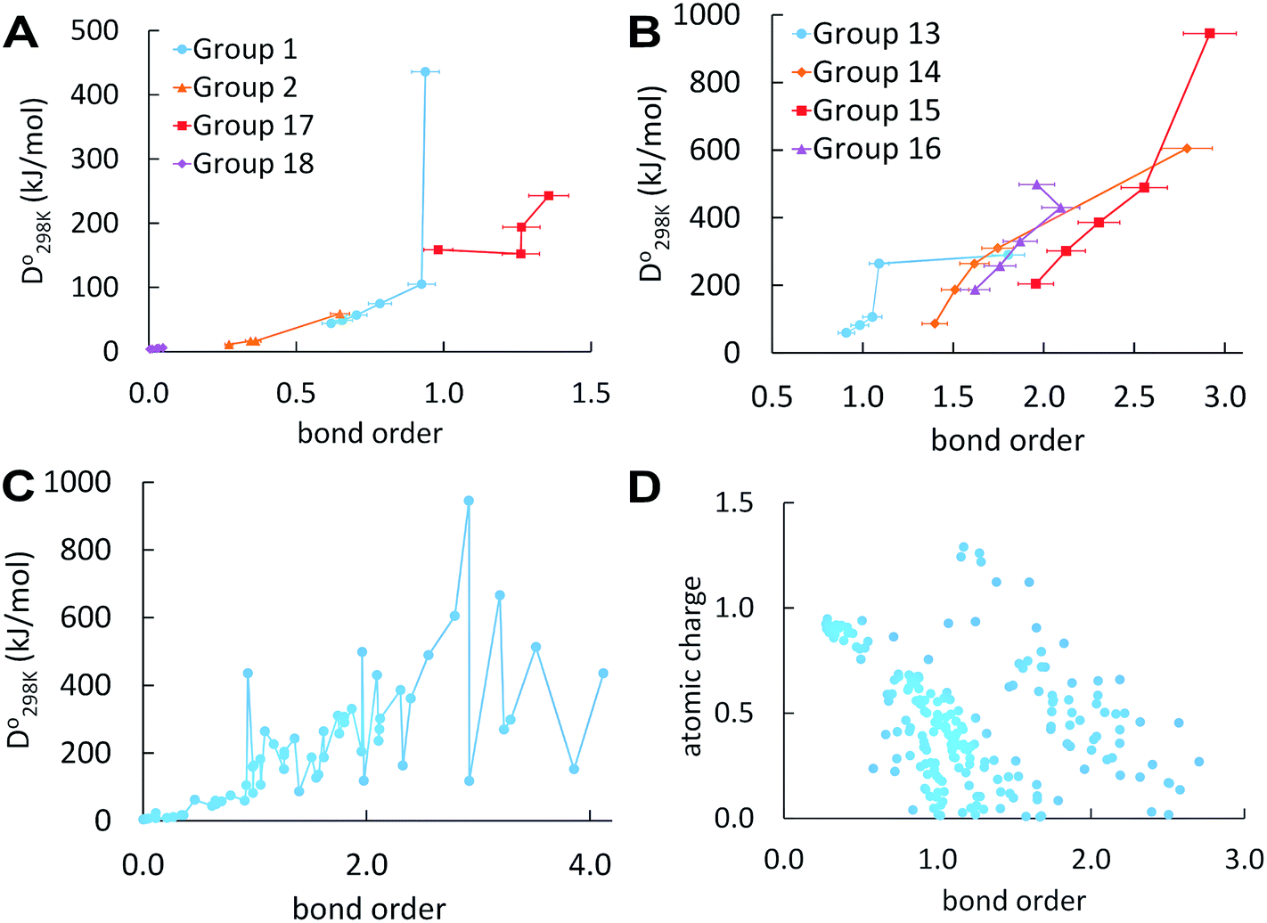 | ||
| Fig. 1 (A) and (B) Bond order versus bond energy for homodiatomics of each main group; (C) bond order versus bond energy for all homodiatomics studied; (D) bond order versus atomic charge magnitude for all heterodiatomics studied. These plots do not include any diatomic ions. | ||
In a recent study of polyatomic molecules and porous solid catalysts, Rohling et al. demonstrated correlations between DDEC6 bond orders and Crystal Orbital Hamilton Populations (COHP).31 These correlations between density-based bond orders and orbital-based bond energies occurred only within families of chemically related structures.31 Those results as well as results of the present paper show bond orders are correlated to bond energies within families of sufficiently similar materials, but not necessarily across different bond types or vastly different materials.
From Table 1, the BOs of halogen dimers peak at Cl2. This trend is consistent with the dissociation energy trend (see Table S2 of ESI†). We hypothesized this effect comes from exchange polarization. We first performed Hartree–Fock (HF) calculations to determine whether this effect comes from electron exchange or correlation. HF yields BO of 1.10 for F2 and 1.38 for Cl2 showing the effect comes from electron exchange not correlation. We then removed different polarization functions from the def2QZVPPD basis set and reran the HF calculations. In all of these calculations, the bond length was re-optimized at each level of theory. Removing d functions yielded BO of 0.95 for F2 and 1.01 for Cl2. Removing both g and f functions yielded BO of 1.07 for F2 and 1.31 for Cl2. With all d, f, and g functions removed, the BOs were 0.92 for F2 and 0.93 for Cl2, which are almost identical. This shows the effect mainly comes from the d functions but f and g functions also contribute. These tests confirmed our theory that the peak of BO and dissociation energy at Cl2 is due to exchange polarization. Similar tests cannot be performed for Br2 and I2, because their d electrons prevent removing d basis functions. Moreover, the Laplacian of the electron density (∇2ρ) is positive at the bond midpoint for F2 but negative for Cl2.32
Table 2 summarizes results for selected diatomic ions. The BO of H2+ was discussed in detail in an earlier work.2 The calculated DDEC6 BOs of HO− and CN− are slightly greater than their heuristic BOs of 1 and 3, respectively. The BOs for CN+ and BC− singlets, which are isoelectronic to singlet C2, are modestly lower and higher than the C2 bond order, respectively. These effects can be attributed to electron cloud contraction towards the atomic nuclei in a cation and electron cloud expansion away from the atomic nuclei in an anion compared to a similar uncharged diatomic. This effect arises, because the outermost electron is usually more tightly bound in a cation than in an anion. This often causes the Manz BO of a diatomic cation (anion) to be smaller (larger) than the heuristic BO. This effect was most pronounced for the hypochlorite anion, which has a computed DDEC6 BO of 1.74 compared to the heuristic BO of 1. As discussed in Section 2.5 below, this unusual BO for ClO− is also due to π-orbital shape-shifting that affects the Virial equilibrium between kinetic and potential energies during bonding.
We investigated relativistic effects including spin–orbit coupling. For selected diatomics, relativistic all-electron calculations were performed in Gaussian09 (ref. 33) near the complete basis set limit using the 4th order Douglas–Kroll–Hess34 Hamiltonian with spin–orbit coupling (DKHSO) and a Gaussian nuclear charge model.35 These were performed using the PBE36 exchange–correlation functional and a universal Gaussian basis set (MUGBS37). Manz reported these calculations for 26 diatomics and compared their bond lengths and BOs to those computed using the CCSD method with relativistic effective core potentials (RECPs) and non-relativistic valence electrons.2 Here, we extend these calculations to Tl2, Pb2, Bi2, Po2, At2, and Rn2. Table S4 of ESI† shows the PBE/MUGBS calculations with DKHSO gave bond lengths 2.8% longer on average (and BOs 11% lower on average) than CCSD/def2QZVPPD for these six homodiatomics. A PBE/MUGBS calculation using DKHSO was also performed for W2 (see Section 2.2). Because CCSD calculations including DKHSO were not available in the Gaussian16 program, we had to choose between the more accurate exchange–correlation theory (i.e., CCSD vs. PBE) and whether to use DKHSO.
2.2 Bond order component analysis (BOCA)
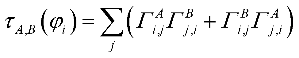
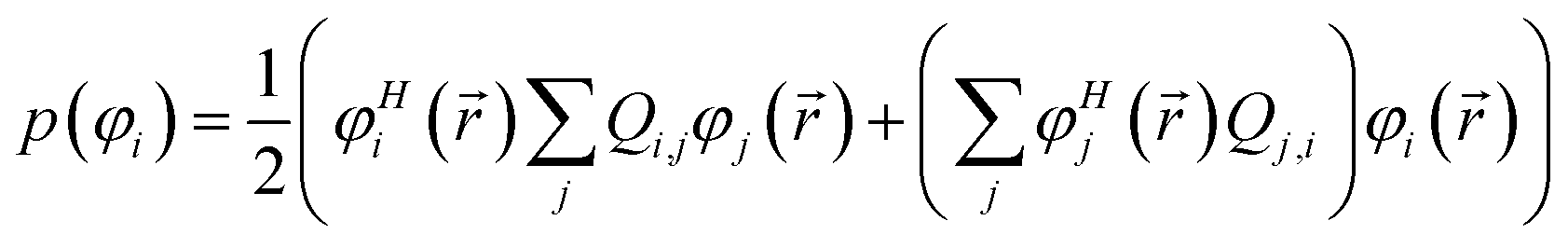
Controversy surrounding BOs arises from the fungible role orbitals play in quantum chemistry. On the one hand, orbitals are useful for chemical interpretation and prediction (e.g., orbital hybridization38 and Woodward–Hoffmann rules39). On the other hand, orbitals depend on the chosen calculation method. Two quantum chemistry calculations describing the same multi-electronic state may have dramatically different orbitals, and even different orbital sets can be constructed to describe the same quantum chemistry calculation.26 Any unitary transformation of the orbitals does not change the system's energy or electron density. Because correlated wavefunction (e.g., CAS-SCF, CCSD, SAC-CI) and density functional theory (DFT) approaches can have different orbital occupancies and different first-order density matrices producing equivalent electron density and system energy, BOs should be defined in a way that does not depend on individual density matrix components or eigenstates.2How can this paradox be resolved in a meaningful way that acknowledges both the usefulness and inherent limitations of orbitals in chemistry? By introducing bond order component analysis (BOCA) that: (a) expresses bond order BA,B for atoms in a material as a functional of the material's electron and spin density distributions via eqn (2) with no explicit orbital dependence and (b) assigns a bond order component BA,B(φi) to each spin-orbital φi so the sum over all spin-orbitals recovers the BO:
 | (4) |
This resolves the paradox by making the BO independent of orbital representation, while simultaneously assigning bond order components (BOCs) to orbitals. Using first-principles reasoning, we now show that BA,B(φi) can be expanded as the sum of an exchange interference term and an exchange non-interference term.
 | (5) |
Using the Pauli spin notation, the ith spin-orbital has the form
 | (6) |
![[r with combining right harpoon above (vector)]](https://www.rsc.org/images/entities/i_char_0072_20d1.gif) ) is the spin-up (alpha) component and φ②i() is the spin-down (beta) component of the spin-orbital. Let {
) is the spin-up (alpha) component and φ②i() is the spin-down (beta) component of the spin-orbital. Let {![[small phi variant, Greek, macron]](https://www.rsc.org/images/entities/i_char_e0d7.gif) i()} be the natural spin-orbitals (NSOs) (i.e., eigenvectors of the first-order density matrices) and {γi} be the NSO occupancies (i.e., eigenvalues of the first-order density matrices). Then define the atomic overlap matrix (AOM) for atom A as
i()} be the natural spin-orbitals (NSOs) (i.e., eigenvectors of the first-order density matrices) and {γi} be the NSO occupancies (i.e., eigenvalues of the first-order density matrices). Then define the atomic overlap matrix (AOM) for atom A as
 | (7) |
 | (8) |
to the nuclear position of atom B's image. Herein, * denotes complex conjugation and superscript H denotes the transposed complex conjugate (aka Hermitian conjugate). Here, summation over B, L means summation over all atoms in the unit cell {B} and their periodic images (if any) {L}. The total electron density is partitioned using
 | (9) |
Different definitions of wA(rA) define different Stockholder-type charge partitioning schemes. Here, we use the DDEC6 charge partitioning method.2,5,7 Then define
 | (10) |
By definition, a unitary matrix U has the properties
 | (11) |
 | (12) |
), and j() do not depend on time. This unitary transforms ![[capital Gamma, Greek, macron]](https://www.rsc.org/images/entities/i_char_e0ba.gif) A into ΓA = U*AUT. The occupancy-weighted electron exchange between compartments A and B from φi to all spin-orbitals is
A into ΓA = U*AUT. The occupancy-weighted electron exchange between compartments A and B from φi to all spin-orbitals is
 | (13) |
The contact exchange assigned to φi is
 | (14) |
 | (15) |
 is the four-vector formed from the spherically averaged electron density (ρavgA(rA)) and spin-magnetization density vector
  assigned to atom A.2 ρ→avg() is the sum of these four-vectors over all atoms in the material. As previously explained,
  are defined using density-derived electrostatic and chemical (DDEC) partitioning.2
The scaling factors
| κA,B = max(min(BA,B/τA,B, 1), 0) | (16) |
| ηA,B = (BA,B − κA,BτA,B)/CEA,B | (17) |
This BOCA assigns BOCs to any desired set of orbitals that can be expressed as a unitary transformation of the NSOs. For small molecules, NSOs are often convenient. For medium and large systems, orbitals localized via unitary transformation (e.g., Pipek–Mezey, Foster–Boys, Edmiston–Ruedenberg, etc.) provide more concise descriptions of bonding interactions.40 Modern variants of Pipek–Mezey localization41,42 are especially useful to quantify individual σ, π, and δ-bonding contributions.
Fig. 2A displays the NSOs, their occupancies, and their BOCs for the carbon dimer, C2. (Here, we adopted the convention of labeling the first valence orbital (rather than the core orbital) as 1σg.15) The 1σg, 1σu, and 2σg orbital shapes show strong s–p mixing. Four NSOs had significantly positive BOCs. The 1πu,x and 1πu,y components (BA,B(φi) = 0.786) were larger than the 1σg component (BA,B(φi) = 0.667) which was larger than the 1σu component (BA,B(φi) = 0.407). The 2σg orbital had negligible BO contribution (BA,B(φi) = 0.045). These bond order components sum to BO = 2.727. Our findings are in agreement with a carbon dimer bond order of 2–3 caused by four bonding components (i.e., two smaller σ-bonding components and two larger π-bonding components) reported by several research groups as discussed by Hermann and Frenking.16
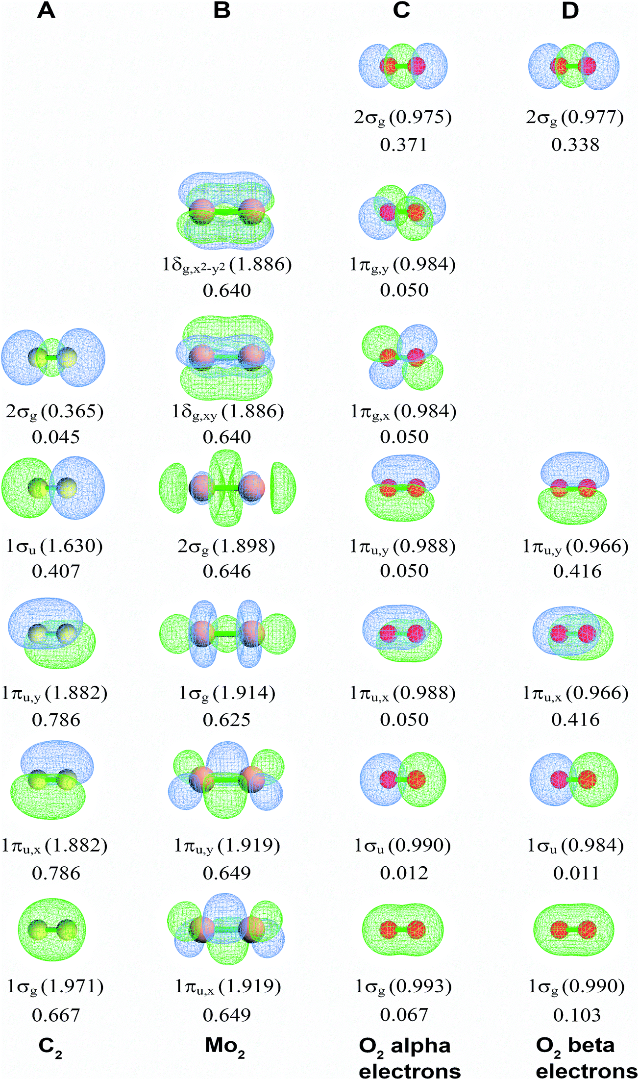 | ||
| Fig. 2 Bond order component analysis (BOCA) for C2 (singlet), Mo2 (singlet), and O2 (triplet) molecules using the natural spin-orbitals. Orbital occupancies are given in parentheses. Bond order components are listed without parentheses. | ||
Fig. 2B displays corresponding information for Mo2. Six NSOs (two π, two σ, and two δ) have nearly equal BOCs (BA,B(φi) = 0.625–0.649) to give BO = 4.120. The π and δ NSOs are pure d hybrids, while the σ NSOs hybridize the dz2 orbital with s and/or pz orbitals. Table 3 lists BOCA for Cr2 having BO = 3.858, which has similar BOCs to Mo2. High BOs of Cr2, Mo2, and some other transition metal dimers attracted considerable interest in prior research.10,43 A CASPT2 study by Roos et al. investigated Cr2, Mo2, W2, Ac2, Th2, Pa2, and U2 estimating BOs of 3.5 (Cr2) and 5.2 (Mo2) using the NSO occupancy bond index (OBI),10 which is often not as precise as the Manz BO.2
| Cr2 | ||
|---|---|---|
| occ. | BOC | |
| Core | 35.87 | 0.168 |
| 1πx,u | 1.91 | 0.608 |
| 1πy,u | 1.91 | 0.608 |
| 1σg | 1.91 | 0.601 |
| 2σg | 1.89 | 0.606 |
| 1δg,xy | 1.89 | 0.598 |
| 1δg,x2−y2 | 1.89 | 0.598 |
| Other | 0.73 | 0.071 |
| Total | 48 | 3.858 |
Wang et al. used the NSO OBI to study the Group 6 homodiatomics Cr2, Mo2, W2, and Sg2.43 They identified an electronic state change from W2 to Sg2 that causes a substantial reduction in the bond order compared to earlier Group 6 homodiatomics.43 Specifically, in Sg2 the 1σu (anti-bonding) orbital becomes doubly occupied by vacating one of the 1δg (bonding) orbitals.43 Our computations showed singlet W2 is near such a transition. Specifically, our CCSD/SDD calculation for W2 converged to a state with filled 1σu (anti-bonding) orbital, which yielded bond length (B.L.) = 2.235 Å and DDEC6 BO = 3.194. Our PBE/MUGBS calculation with 4th order Douglas–Kroll–Hess Hamiltonian and spin–orbit coupling converged to a state with empty 1σu (anti-bonding) orbital (similar to Mo2 and Cr2), which yielded B.L. = 2.017 Å and DDEC6 BO = 3.842. Therefore, the BO of W2 has substantial uncertainty.
The anti-bonding versus bonding characteristic of an orbital cannot be assigned based on whether the orbital has positive or negative bond order component BA,B(φi) which is based on electron exchange. As an example, consider a homodiatomic AB that contains only one occupied orbital, with equivalent electron density distributions on both atoms. Since there are no other occupied orbitals and the orbital self-exchange over each atom is ½, then τA,B(φi) = 2(½)(½) = ½ independent of whether the orbital is bonding or anti-bonding. Hence, both bonding and anti-bonding orbitals may have positive values of BA,B(φi).
Fig. 2C and D display alpha and beta results for O2 (calculated BO = 1.962) in the spin-polarized triplet state (S = 1, SZ = 1). Here, the alpha NSOs diagonalize the alpha density matrix, and the beta NSOs diagonalize the beta density matrix. This molecule presents a natural experiment showing that occupying an anti-bonding orbital decreases the BOC of the associated bonding orbital. This cancellation occurs because electron exchange between a bonding orbital and the corresponding anti-bonding orbital is out-of-phase with the bonding orbital's self-exchange. The spin-up (alpha) electrons occupy both the π-bonding (1πu,x and 1πu,y) and π-anti-bonding orbitals (1πg,x and 1πg,y), while the beta electrons occupy the π-bonding but not the π-anti-bonding orbitals. The four π-orbitals have negligible BOCs for the alpha electrons (BA,B(φi) = 0.050), while the two π-bonding orbitals have large BOCs for the beta electrons (BA,B(φi) = 0.416). The 1σg and 1σu orbitals showed little s-p mixing leading to almost full bonding-antibonding cancellation (net BOC = 0.079 for alpha and 0.114 for beta). Accordingly, the 2σg orbital shows substantial bonding (0.371 for alpha and 0.338 for beta).
2.3 Three ways semicore electrons affect valence electron bonding
Semicore electrons fill subshells one level deeper than the corresponding valence subshells. They are more diffuse than core electrons but not as diffuse as valence electrons. Semicore electrons have three effects on valence electron bonding.First, core and semicore electrons electrostatically screen valence electrons from the nuclear charge. It is common knowledge that s subshell electrons have nonzero density at the nucleus, while p, d, and f subshell electrons have zero density at the nucleus. Consequently, the s subshell valence electrons are less shielded and less diffuse than p, d, or f subshell electrons having the same principle quantum number.
Second, semicore electrons most efficiently screen valence electrons from the same subshell type (e.g., s semicore screening s valence, p semicore screening p valence). This is due to the similar angular dependence of orbitals having same subshell type. This causes the inaugural subshell effect in which the first valence subshell of any type (i.e., 1s, 2p, 3d, 4f) is comparatively less diffuse, because there is no corresponding semicore subshell of the same type. This has profound and widespread effects on chemical bonding. 3d valence electrons are more localized than 4d and 5d valence electrons, as manifested by local magnetic moments for many 3d elements, while the 4d and 5d elements are less prone to magnetism.44 (Among d-block pure element solids in their lowest energy phases, bulk Cr is anti-ferromagnetic, bulk Mn has non-collinear magnetism, bulk Fe and Co and Ni are ferromagnetic, and all others are non-magnetic or paramagnetic.45) Similarly, many 4f elements develop local magnetic moments.44 In main group chemistry, the 2p elements are special, because the 2s and 2p orbitals have similar effective radii, which promotes strong s–p hybridization.46 In contrast, the 3p orbital effective radius is much larger than the 3s orbital effective radius, leading to lesser s–p hybridization for period 3 (and heavier) elements compared to period 2 elements.46
Third, diffuse semicore electrons make the dressed-exchange hole less diffuse in the bonding region, leading to smaller BOs. Because the dressed-exchange hole  integrates to exclude exactly one electron, any positive semicore density near position must result in
  decreasing farther away from .2 The BO depends on the dressed-exchange hole delocalization factor ΛA,B (see eqn (2) and (3)). Thus, making the dressed-exchange hole less delocalized decreases the BO.2 Multiple-order bonds have shortened bond lengths compared to a single-order bond between the same pair of elements. Thus, density overlap between semicore and valence electrons and the corresponding BO weakening effect will be larger for multiple-order bonds than for a single-order bond between the same pair of elements. Consequently, chemical elements with diffuse semicore electrons often prefer single-order bonds to multiple-order bonds. For this reason, multiple-order bonds are less common for heavier elements than for lighter elements in Groups 13–16.47
Examining Table 1, homodiatomic BOs systematically decrease down most of the main chemical groups except the halogens, noble gases, and alkaline earths. The halogens have already been discussed above. Dispersion bonding in the noble gas homodiatomics increases with atomic number. Fig. 3 quantifies (semi-)core electron diffuseness for Groups 1–2 and 13–17. This data supports the following observations. For alkaline earths (Group 2), there is a strong jump in semicore electron diffuseness from Be2 to Mg2 with corresponding huge BO decrease from 0.648 to 0.281, with smaller changes from Mg2 to Ca2 to Sr2. Both the BO and the dissociation energy (see Table S2 of ESI†) show a minimum at Mg2. Many authors investigated vibrational and excitation modes of alkaline earth homodiatomics.48–50 For Groups 13–14, the large decrease in BO from period 2 to 3 is not accompanied by increased semicore electron diffuseness, but should be attributed to electronic state changes. In Group 14, C2 is a spin singlet while Si2, Ge2, and Sn2 are spin triplets. In Group 13, B2 and Al2 are both triplets, but have different orbital angular momenta; the term symbols are 3Σg− for B2 and 3Πu for Al2.28 The subsequent gradual BO decrease from periods 3 to 4 to 5 of these groups can be attributed to increased semicore electron diffuseness. For Groups 1 and 15, the BO steadily decreases from period 2 to 3 to 4 to 5. In Group 15, the inaugural subshell effect causes an enhanced BO decrease between periods 2 and 3. GVB calculations showed the bonding electrons become less perfectly paired when going from N2 to P2 to As2.51 Groups 16–17 have less diffuse semicore electrons than Group 15; this results in less BO weakening when going down these groups compared to Group 15. The slight increase in computed BO from O2 to S2 is not statistically significant, because it is within the ±5% chemical accuracy of the method.2
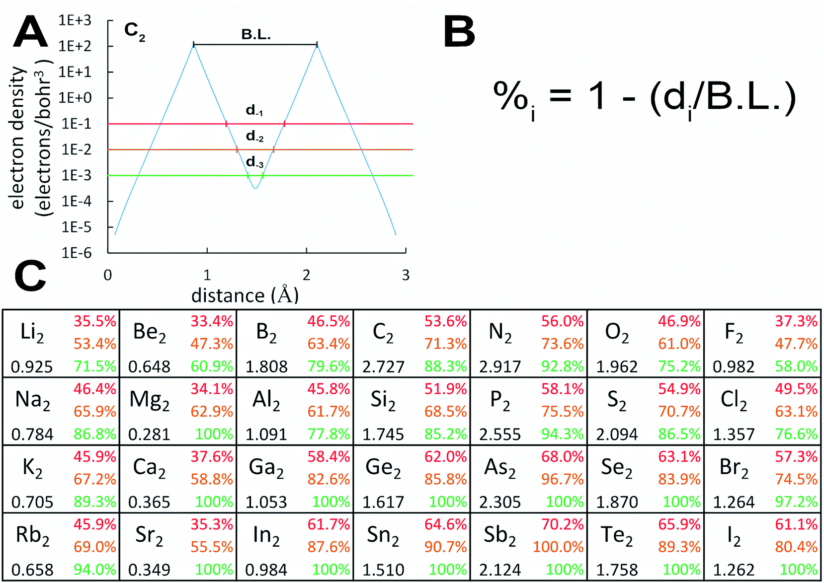 | ||
| Fig. 3 Graphic showing diffuse semicore electrons decrease the bond order. (A) Plot of core electron density versus distance along the C–C axis in C2. The red, brown, and green lines demarcate the 10−1, 10−2, and 10−3 e bohr−3 electron density thresholds corresponding to the distances d−1, d−2, and d−3, respectively. (B) Formula used to compute the percentage of the bond length for which the (semi-)core electron density is above each threshold (aka ‘(semi-)core percentages’). (C) Partial periodic table (periods 2–5 and groups 1–2, 13–17) showing trends in the bond orders (black) and (semi-)core percentages corresponding to the respective density thresholds (red, brown, and green). | ||
BO changes when going down these groups are not straightforwardly attributable to s–p mixing changes. Fig. 4 shows s–p mixing is strong for both the light and heavy elements of Groups 1–2 and 13–15 but not 16–18. Because Groups 1–2 and 13–14 contain an unoccupied 2σg orbital, s–p mixing will occur in the 1σg orbital to increase the density concentration in the space between the two atoms. Because the 1σg and 2σg orbitals are orthonormal and comprised of the s and p atomic orbitals, s–p mixing has negligible impact on the total electron density distribution when both the 1σg and 2σg orbitals are fully occupied (i.e., Groups 15–18). Since any linear combination of fully occupied 1σg and 2σg orbitals is nearly an eigenstate of the first-order density matrix for Groups 15–18, the fully occupied 1σg and 2σg orbitals can be chosen arbitrarily to either have or not have s–p mixing. When 2σg is mostly unoccupied, s–p mixing in the 1σu orbital is largely driven by minimizing the magnitude of the negative exchange interference term in BOCA between occupied 1σu and 1σg orbitals. When both the 1σg and 2σg orbitals are nearly fully occupied, the total exchange interference term between these two orbitals and the 1σu orbital is insensitive to s–p mixing. Therefore, s–p mixing is not meaningful for Groups 15–18.
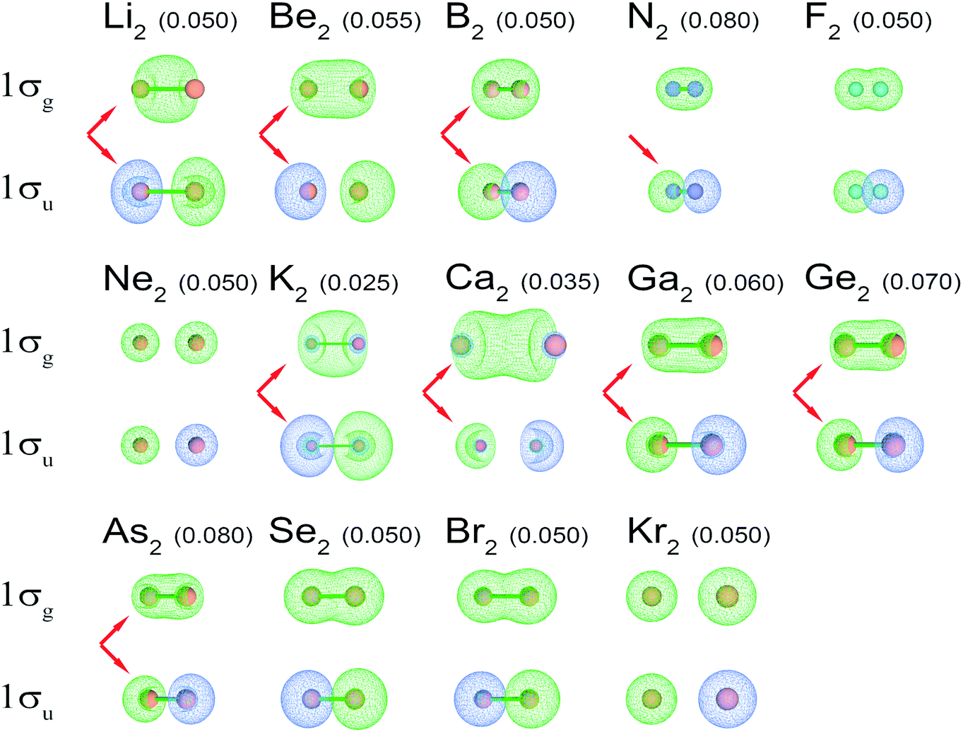 | ||
| Fig. 4 1σg and 1σu NSOs for high-level quantum chemistry calculations of period 2 and 4 main-group homodiatomics. (The C2 and O2 orbitals are shown in Fig. 2.) The arrows indicate orbitals showing strong s–p mixing. S–p mixing is visible in a 1σg orbital as pockets intruding into the two ends of the orbital. S–p mixing is visible in the 1σu orbital as pockets intruding into the lobe centers. Numbers in parentheses are the orbital contour values in atomic units. For each molecule, the contour value was chosen to maximize visual clarity. | ||
2.4 Learning aids for chemistry education
Most importantly, a spin-orbital cannot be classified as bonding versus anti-bonding based on its BOCs. We propose the bonding versus anti-bonding characteristic describes the difference in overall performance between two states, while BOCs quantify the particular division of message transmission within one state. Using the computer network analogy, a channel is classified as ‘anti-bonding’ if adding this channel to the network actually decreases overall message transmission throughout the network. We introduce a collaboration index (CI) quantifying change in network throughput. We define a spin-orbital or network channel as bonding (anti-bonding) if the CI is positive (negative) and non-bonding if it is zero. Consider a network comprised of two elementary channels, called Red and Blue, that simultaneously transmits 0.8 messages over the Red channel and 0.7 over the Blue channel to give 1.5 simultaneous transmissions. Suppose that adding channel Green results in a new network state with 0.25 messages simultaneously transmitted over the Green channel, 0.53 over the Red channel, and 0.42 over the Blue channel to give 1.2 simultaneous transmissions. Because the CI = 1.2–1.5 = −0.3 is negative, the Green channel is anti-bonding. This is true even though the Green channel transmitted 0.25 messages simultaneously, which is analogous to a positive BOC.
Period 2 homodiatomics (Li2, Be2, B2, C2, N2, O2, F2, and Ne2) could potentially be an ideal series to teach BOs in chemistry textbooks. DeKock and Gray discuss this series with quantitative heuristic BOs for Li2, N2, O2, F2, and Ne2, but semi-quantitative heuristic BOs of 0–1 for Be2, 1–2 for B2, and 2–3 for C2 using an s–p mixing argument.15 MO diagrams without s–p mixing are notoriously wrong (i.e., predicting BOs of 0 for Be2, 1 for B2, and 2 for C2).15 Even though the MO diagram for Li2 without s–p mixing gives the correct heuristic BO = 1, this molecule has strong s-p mixing (see Fig. 4) which also yields a heuristic BO = 1.
Table 4 lists heuristic molecular orbitals for the period 2 homodiatomics. Each molecular orbital must be multiplied by a normalization constant that is of order unity. In the spirit of idealized simplicity, this heuristic model uses whole number NSO occupancies. For the period 2 homodiatomics, eight valence NSOs are of interest: 1σg, 1σu, 1πx,u, 1πy,u, 2σg, 1πx,g, 1πy,g, 2σu. Here, the prefix 1 or 2 denotes the first or second valence NSO of that symmetry type. Our detailed quantum chemistry calculations presented in this article confirmed these NSOs fill in the order listed.
| M.O. | Expansion in atomic orbitals | C.I. | Molecule | Heuristic BO |
|---|---|---|---|---|
| a The 1πx,u and 1πy,u orbitals are half-filled.b The 1πx,u and 1πy,u orbitals are filled.c The 1πx,g and 1πy,g orbitals are half-filled.d The 1πx,g and 1πy,g orbitals are filled. | ||||
| Core | — | 0 | — | 0 |
| 1σg | ((√3sA + pzA) + (√3sB − pzB))/(2√2) | 1 | Li2 | 1 |
| 1σu | ((√3sA − pzA) − (√3sB + pzB))/(2√2) | −¼ | Be2 | ¾ |
| 1πx,u, 1πy,u | (pxA + pxB)/√2, (pyA + pyB)/√2 | 1 | B2a | 1¾ |
| 1πx,u, 1πy,u | (pxA + pxB)/√2, (pyA + pyB)/√2 | 1 | C2b | 2¾ |
| 2σg | ((sA − √3pzA) + (sB + √3pzB))/(2√2) | ¼ | N2 | 3 |
| 1πx,g, 1πy,g | (pxA − pxB)/√2, (pyA − pyB)/√2 | −1 | O2c | 2 |
| 1πx,g, 1πy,g | (pxA − pxB)/√2, (pyA − pyB)/√2 | −1 | F2d | 1 |
| 2σu | ((sA + √3pzA) − (sB − √3pzB))/(2√2) | −1 | Ne2 | 0 |
Each of the eight valence NSOs are expanded as a linear combination of atom-in-material (AIM) orbitals. Here, the AIM orbitals are not those of isolated atoms, but rather those of atoms in the material which are effected by the molecular environment. For example, an atomic s orbital in the molecule might be less diffuse than that for the isolated atom.52 As defined herein, each AIM orbital is orthogonal to all other AIM orbitals on the same atom, but not to AIM orbitals on other atoms. In the orbital composition, superscripts A and B refer to atomic orbitals from the first and second atoms, respectively. For the diatomics, the origin is placed at atom A's nuclear position, and atom B is located along the positive z-axis. Methods for computing AIM orbitals from a quantum-mechanically computed first-order electron density matrix have been described in the literature,53–55 but here we do not require such an explicit computation. Within the natural atomic orbital (NAO) and natural bond orbital (NBO) formalism, the AIM orbitals described here would be analogous to the pre-NAOs since pre-NAOs on the same atom are orthogonal while those on different atoms are not.54,56 The π-orbitals are the easiest to expand, because they have negligible s–p mixing.
Computations showed there is substantial s–p mixing in the σ-orbitals. As shown in Fig. 4, this is true even for Li2 in which 1σg is the only valence orbital nearly fully occupied. S–p mixing lowers the energy of this 1σg orbital by concentrating electron density between the two atoms (see Fig. 4). For period 2 atoms, the s and p orbitals have similar effective radii.46 Each p orbital has a maximum amplitude that is √3 times that of the s orbital amplitude.38
The kinetic energy of an orbital is sensitive to how many phase changes the orbital has and how abruptly these phase changes occur. To make the orbital energetics most favorable, the number of phase changes and their abruptness should be minimized.
Fig. 5 plots the s–p atomic hybrid whose unnormalized value along the z-axis is
 | (18) |
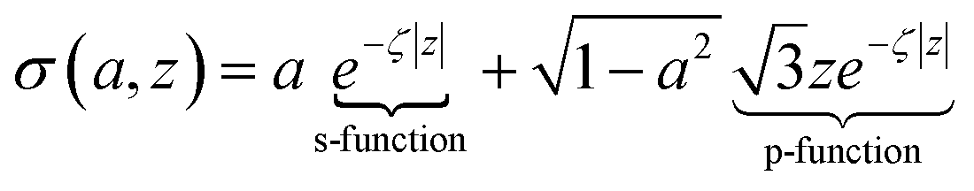
 , as shown in the red curve in Fig. 5. Hence, the quantity of s–p mixing for the 1σg and 1σu orbitals of the period 2 homodiatomics can be estimated by noting the similar s and p orbital radii and setting the atomic hybridized orbital value to zero at either ζ|z| = −1 or +1. This clearly yields √3
![[thin space (1/6-em)]](https://www.rsc.org/images/entities/char_2009.gif) :1 for the s:pz ratio in these orbitals. The s:pz ratios for the 2σg and 2σu orbitals then straightforwardly follows from the requirement that these orbitals be orthogonal to the 1σg and 1σu orbitals. For period 3 and beyond, the valence p-orbitals have substantially larger effective radius than the valence s-orbital, and this alters the amount of s–p mixing compared to the period 2 atoms.46
:1 for the s:pz ratio in these orbitals. The s:pz ratios for the 2σg and 2σu orbitals then straightforwardly follows from the requirement that these orbitals be orthogonal to the 1σg and 1σu orbitals. For period 3 and beyond, the valence p-orbitals have substantially larger effective radius than the valence s-orbital, and this alters the amount of s–p mixing compared to the period 2 atoms.46
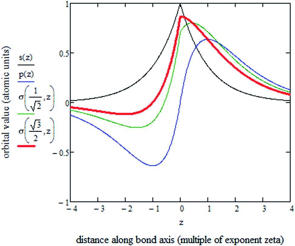 | ||
| Fig. 5 Plot of s-orbital (black), p-orbital (blue), and two s–p hybrids along the z-axis of a single atom. A s–p hybrid with equal coefficients of s and p orbitals is shown in green. The s–p hybrid (red) with (√3sA + pzA)/2 is approximately optimal, because it has a value of zero at zζ = −1. | ||
Table 4 also lists the CI for each heuristic NSO. Restricted to diatomic molecules, the collaboration index (CI) was estimated from scaled phase overlaps between the AIM orbital component products:
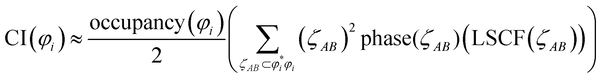 | (19) |
 refers to the coefficient of an interatomic AIM orbital product occurring within
  . The lobe size change factor (LSCF) equals one for the period 2 homodiatomics; its meaning will be discussed in Section 2.5 below. The (ζAB)2 occurs in eqn (19), because mathematically this yields a purely in-phase CI = 1 for a doubly occupied orbital irrespective of the amount of s–p mixing. Consider the generalized 1σg = ((√fsA + √(1 − f)pzA) + (√fsB − √(1 − f) pzB))/(√2), where 0 ≤ f < 1 controls the s–p mixing. Evaluating eqn (19) for this orbital (which has all in-phase overlaps) yields CI = f2 (for (sAsB) term) + f(1 − f) (for sApzB term) + (1 − f)f (for pzAsB term) + (1 − f)2 (for pzApzB term) = 1 independent of the f value. The 1σu orbital has some in-phase and some out-of-phase overlaps. Expanding (1σu)2 = (((√3sA − pzA) − (√3sB + pzB))/(2√2))2 = ⅜(sAsA) − √3/4 (sApzA) + ⅛(pzApzA) + ⅜(sBsB) + √3/4(sBpzB) + ⅛(pzBpzB) − ¾(sAsB) − √3/4(sApzB) + √3/4(pzAsB) + ¼(pzApzB). (pzApzB) is out-of-phase since the positive lobe of pzA overlaps the negative lobe of pzB. Since (sAsB) is in-phase, then −(sAsB) must be out-of-phase. (pzAsB) is in-phase since the positive lobe of pzA overlaps the positive lobe of sB. Since (sApzB) is out-of-phase (i.e., positive lobe of sA overlaps negative lobe of pzB), then −(sApzB) is in-phase. Hence, CI(1σu) = −((¾)2) + (√3/4)2 + (√3/4)2 − (¼)2 = −¼.
We computed the heuristic BO for each period 2 homodiatomic as the sum over orbitals of orbital CI value times orbital occupancy. We then performed BOCA (eqn (4)–(17)) using these heuristic orbitals and heuristic BOs as input, which yielded ηA,B = 0. This heuristic BOCA approximated the overlap ![[S with combining tilde]](https://www.rsc.org/images/entities/i_char_0053_0303.gif) i,jA of the AIM orbitals i and j as 1 if i = j and AIM orbital i is centered on atom A and 0 otherwise. Table 5 gives the heuristic BOCA and Table S5 of ESI† gives the accurate QM-calculated BOCA for these homodiatomics. Because two NSOs of the same symmetry group having equal occupancies can be mixed to form equally valid NSOs of the same symmetry group, comparisons are most meaningful for orbital symmetry groups. As shown in Table 6, the heuristic and QM-calculated BO components for each orbital symmetry group are in fair agreement, while the heuristic and QM-calculated BOs are in excellent agreement. This excellent agreement means the Be2, B2, and C2 bond orders are finally understood.
i,jA of the AIM orbitals i and j as 1 if i = j and AIM orbital i is centered on atom A and 0 otherwise. Table 5 gives the heuristic BOCA and Table S5 of ESI† gives the accurate QM-calculated BOCA for these homodiatomics. Because two NSOs of the same symmetry group having equal occupancies can be mixed to form equally valid NSOs of the same symmetry group, comparisons are most meaningful for orbital symmetry groups. As shown in Table 6, the heuristic and QM-calculated BO components for each orbital symmetry group are in fair agreement, while the heuristic and QM-calculated BOs are in excellent agreement. This excellent agreement means the Be2, B2, and C2 bond orders are finally understood.
| M.O. | Li2 | Be2 | B2 | C2 | N2 | O2 | F2 | Ne2 | ||||||||
|---|---|---|---|---|---|---|---|---|---|---|---|---|---|---|---|---|
| occ | BOC | occ | BOC | occ | BOC | occ | BOC | occ | BOC | occ | BOC | occ | BOC | occ | BOC | |
| Core | 4 | 0 | 4 | 0 | 4 | 0 | 4 | 0 | 4 | 0 | 4 | 0 | 4 | 0 | 4 | 0 |
| 1σg | 2 | 1 | 2 | ⅜ | 2 | 21/40 | 2 | 33/56 | 2 | ¾ | 2 | ¾ | 2 | ¾ | 2 | 0 |
| 1σu | 0 | 0 | 2 | ⅜ | 2 | 21/40 | 2 | 33/56 | 2 | 0 | 2 | 0 | 2 | 0 | 2 | 0 |
| 1πx,u | 0 | 0 | 0 | 0 | 1 | 7/20 | 2 | 11/14 | 2 | 1 | 2 | ½ | 2 | 0 | 2 | 0 |
| 1πy,u | 0 | 0 | 0 | 0 | 1 | 7/20 | 2 | 11/14 | 2 | 1 | 2 | ½ | 2 | 0 | 2 | 0 |
| 2σg | 0 | 0 | 0 | 0 | 0 | 0 | 0 | 0 | 2 | ¼ | 2 | ¼ | 2 | ¼ | 2 | 0 |
| 1πx,g | 0 | 0 | 0 | 0 | 0 | 0 | 0 | 0 | 0 | 0 | 1 | 0 | 2 | 0 | 2 | 0 |
| 1πy,g | 0 | 0 | 0 | 0 | 0 | 0 | 0 | 0 | 0 | 0 | 1 | 0 | 2 | 0 | 2 | 0 |
| 2σu | 0 | 0 | 0 | 0 | 0 | 0 | 0 | 0 | 0 | 0 | 0 | 0 | 0 | 0 | 2 | 0 |
| Total | 6 | 1 | 8 | ¾ | 10 | 1¾ | 12 | 2¾ | 14 | 3 | 16 | 2 | 18 | 1 | 20 | 0 |
| Orbital group | Li2 | Be2 | B2 | C2 | ||||
|---|---|---|---|---|---|---|---|---|
| occ. | BOC | occ. | BOC | occ. | BOC | occ. | BOC | |
| Core | 3.99 (4) | 0.000 (0) | 4.00 (4) | 0.000 (0) | 4.00 (4) | 0.000 (0) | 4.00 (4) | 0.000 (0) |
| 1 & 2σg | 1.85 (2) | 0.865 (1) | 2.03 (2) | 0.362 (⅜) | 2.24 (2) | 0.626 (21/40) | 2.34 (2) | 0.712 (33/56) |
| 1 & 2σu | 0.03 (0) | 0.003 (0) | 1.77 (2) | 0.257 (⅜) | 1.70 (2) | 0.397 (21/40) | 1.64 (2) | 0.409 (33/56) |
| πxu & πyu | 0.12 (0) | 0.056 (0) | 0.12 (0) | 0.022 (0) | 1.94 (2) | 0.773 (7/10) | 3.76 (4) | 1.572 (11/7) |
| πxg & πyg | 0.00 (0) | 0.000 (0) | 0.08 (0) | 0.004 (0) | 0.12 (0) | 0.011 (0) | 0.22 (0) | 0.018 (0) |
| Other | 0.01 (0) | 0.01 (0) | 0.00 (0) | 0.00 (0) | 0.00 (0) | 0.00 (0) | 0.04 (0) | 0.02 (0) |
| Total | 6 (6) | 0.93 (1) | 8 (8) | 0.65 (¾) | 10 (10) | 1.81 (1¾) | 12 (12) | 2.73 (2¾) |
| Orbital group | N2 | O2 | F2 | Ne2 | ||||
|---|---|---|---|---|---|---|---|---|
| occ. | BOC | occ. | BOC | occ. | BOC | occ. | BOC | |
| Core | 4.00 (4) | 0.000 (0) | 4.00 (4) | 0.000 (0) | 4.00 (4) | 0.000 (0) | 4.00 (4) | 0.000 (0) |
| 1 & 2σg | 3.94 (4) | 1.001 (1) | 3.93 (4) | 0.877 (1) | 3.90 (4) | 0.746 (1) | 3.97 (4) | 0.004 (0) |
| 1 & 2σu | 1.98 (2) | 0.029 (0) | 2.01 (2) | 0.027 (0) | 2.07 (2) | 0.025 (0) | 3.97 (4) | 0.004 (0) |
| πxu & πyu | 3.86 (4) | 1.852 (2) | 3.90 (4) | 0.932 (1) | 3.96 (4) | 0.100 (0) | 3.96 (4) | 0.002 (0) |
| πxg & πyg | 0.12 (0) | 0.012 (0) | 2.02 (2) | 0.104 (0) | 3.94 (4) | 0.094 (0) | 3.96 (4) | 0.002 (0) |
| Other | 0.10 (0) | 0.03 (0) | 0.12 (0) | 0.02 (0) | 0.13 (0) | 0.01 (0) | 0.14 (0) | 0.00 (0) |
| Total | 14 (14) | 2.92 (3) | 16 (16) | 1.96 (2) | 18 (18) | 0.98 (1) | 20 (20) | 0.01 (0) |
2.5 Manz bond orders and BOCA incorporate both kinetic and potential energy contributions to bond order
In special relativity, the energy-momentum relationship
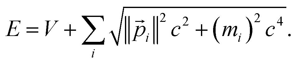 | (20) |
![[p with combining right harpoon above (vector)]](https://www.rsc.org/images/entities/i_char_0070_20d1.gif) i), the speed of light (c), the rest mass of particle i (mi), the system's potential energy (V), and the system's total energy (E). (Adapted from ref. 57 with summation over particles.) For all applications considered herein, the rest mass is constant. In this article, we are primarily interested in time-independent energy eigenstates.
i), the speed of light (c), the rest mass of particle i (mi), the system's potential energy (V), and the system's total energy (E). (Adapted from ref. 57 with summation over particles.) For all applications considered herein, the rest mass is constant. In this article, we are primarily interested in time-independent energy eigenstates.
For such stationary states, the variation in total energy with respect to infinitesimal changes in any variational parameter (χ) is zero:
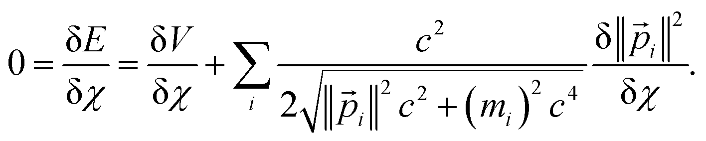 | (21) |
For a trial wavefunction, these variational parameters include any adjustable parameters (e.g., basis set coefficients or scaling parameters) in the trial wavefunction. When the bond length is optimized, then the bond length is also considered to be one of these variational parameters. When the bond length is held constant (i.e., not optimized), then it is not considered to be one of these variational parameters. At the stationary state, potential energy changes with respect to any variational parameter are related to momentum changes with respect to the same variational parameter:
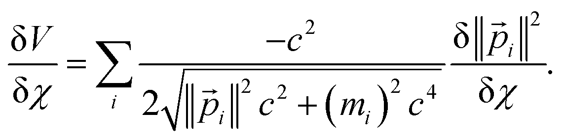 | (22) |
Next, we consider a dilation that acts on both the nuclear positions {![[R with combining right harpoon above (vector)]](https://www.rsc.org/images/entities/i_char_0052_20d1.gif) A′ = A/λ} and the electronic positions {
A′ = A/λ} and the electronic positions {![[e with combining right harpoon above (vector)]](https://www.rsc.org/images/entities/i_char_0065_20d1.gif) i′ = i/λ} to uniformly shrink or enlarge the system:
i′ = i/λ} to uniformly shrink or enlarge the system:
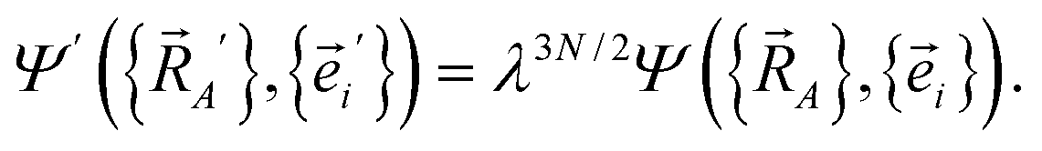 | (23) |
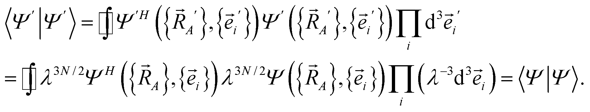 | (24) |
Since the quantum mechanical momentum per particle i is given by
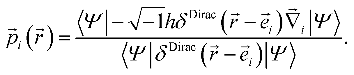 | (25) |
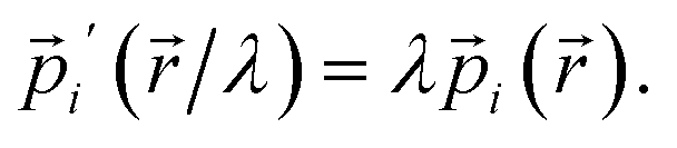 | (26) |
 | (27) |
V′(![[r with combining right harpoon above (vector)]](https://www.rsc.org/images/entities/char_0072_20d1.gif) /λ) ≈ λV() /λ) ≈ λV()
| (28) |
 | (29) |
 | (30) |
These Virial relationships show the P.E. of an energy eigenstate is related to its K.E. Suppose we have a trial wavefunction for which the K.E. is too small in magnitude compared to what is required by the GVR. Using λ > 1, we can shrink this system until it satisfies the GVR, which will increase the magnitude of the K.E. proportional to λ2 and the P.E. magnitude proportional to λ. On the other hand, if the K.E. is too large in magnitude we can dilate the system with λ < 1 to satisfy the GVR. This was already shown many years ago by Lowdin for the nonrelativistic case.58 Here we see it also applies to relativistic quantum chemistry.
This has the following applications to chemical bonding. By the uncertainty principle, the smaller a particle's standard deviation in position, the larger its standard deviation in momentum:59
| σpositionσmomentum ≥ ℏ/2 | (31) |
As described in Section 2.4 above, we can view a molecular orbital (MO) as built from a linear combination of scaled AIM orbitals. When unscaled AIM orbital lobes from neighboring atoms overlap in-phase, they create an unscaled MO that has larger lobes compared to the unscaled AIM orbitals. This enlarged unscaled MO lobe has larger position standard deviation than the parent unscaled AIM orbital lobes, which by the uncertainty principle means this unscaled MO has reduced standard deviation in momentum (and hence lower kinetic energy) than the unscaled AIM orbital lobes. To satisfy the Virial relation, the system must shrink (λ > 1) until the K.E. and P.E. achieve Virial balance. This shrinking reduces the optimized bond length and increases both the P.E. magnitude and K.E. Hence, in-phase (aka ‘bonding’) interactions of AIM orbitals from neighboring atoms leads to shortened bond length and lower overall system energy. Ruedenberg et al. quantified this Virial balancing process for a few diatomics.52,60,61
Out-of-phase overlaps between AIM orbital lobes from neighboring atoms produce the opposite effect. When unscaled AIM orbital lobes from neighboring atoms overlap out-of-phase, they create an unscaled MO that has smaller lobes compared to the unscaled AIM orbitals. This smaller unscaled MO lobe has smaller position standard deviation than the parent unscaled AIM orbital lobes, which by the uncertainty principle means this unscaled MO has increased standard deviation in momentum (and hence higher kinetic energy) than the unscaled AIM orbital lobes. To satisfy the Virial relation, the system must dilate (λ < 1) until the K.E. and P.E. achieve Virial balance. This enlarging increases the optimized bond length and decreases both the P.E. magnitude and K.E. Hence, out-of-phase (aka ‘anti-bonding’) interactions of AIM orbitals from neighboring atoms leads to longer bond length and higher overall system energy.
Electron exchange is a key part of the P.E. changes during chemical bonding. Because the Virial relation is properly between the K.E. and P.E., we can rescale the number of electrons exchanged to describe the P.E. contribution to bond order between two atoms in a material. This is why the Manz bond order is based on a dressed-exchange (i.e., rescaled exchange) rather than on a pure exchange.2 A previously discussed example illustrates this point.2 Consider the H2+ system as the inter-atomic distance is stretched to infinity. When the two atoms are infinitely separated, their total energy equals the sum for an isolated H atom plus an isolated H+ ion; therefore, the bond dissociation energy is zero. The symmetric state, with 0.5 electrons located around each nucleus, is a quantum superposition of the two symmetry broken states: [H …. H+] and [H+ …. H]. All three states have equal energies. The symmetric state has 2(½)(½) = ½ of an electron exchanged between the two atoms with atom self-exchange accounting for the other ¼ + ¼ = ½ electron. The symmetry broken states have one self-exchanged electron on the H atom, zero on the H+ ion, and no electrons exchanged between the two atoms. Consequently, bond indices based on pure electron exchange (e.g., Mayer bond index3,62,63) or delocalization of the exchange–correlation hole across atom pairs (e.g., second-order delocalization index64) give different results for the symmetric and symmetry broken states of H2+, even though their energies are equal. The Manz bond order solves this problem by scaling the exchange contributions (aka dressed-exchange) according to the density overlaps between atoms, which always produces a bond order of zero for non-overlapping atoms.2 This is physically sound, because non-overlapping atoms do not share any in-phase or out-of-phase AIM orbital overlaps.
The Virial relation quantifies overall system changes in K.E. and P.E. The Virial relation does not require these changes to take place within the same MO. Hence, a change in K.E. of one MO could be Virial balanced by a change in P.E. of another M.O. This is crucial to understanding the distinction between the collaboration index (C.I.) based on orbital overlap phase characteristics and the bond order component (BOC) based on dressed-exchange. Specifically, the C.I. quantifies the kinetic-based contribution of each spin-orbital to bond order, while the BOC quantifies the dressed-exchange contribution of each spin-orbital to bond order. By the Virial relation, the total kinetic-based and total dressed-exchange based contributions to bonding are equal, even though these can be distributed differently among the MOs.
Specific examples quantify these concepts. First, we revisit the Mo2 example shown in Fig. 2. Among the six doubly-occupied valence orbitals, the 1δg,x2-y2 and 1δg,xy orbitals show large lobe size increases compared to the parent AIM orbitals. The inner lobes of the 1πu,x and 1πu,y orbitals also show larger sizes due to in-phase AIM orbital overlaps. In contrast, the 1σg and 2σg orbitals show negligible lobe size increase compared to the parent AIM orbitals. This demonstrates the need for a Lobe Size Change Factor (LSCF) to be included in eqn (19) when computing the C.I. This LSCF should be ∼1 when in-phase (out-of-phase) AIM orbital overlaps lead to substantially increased (decreased) lobe sizes, but ∼0 when the AIM orbital overlaps have negligible effect on the lobe size. With this inclusion, the C.I. would be ∼0 for the 1σg and 2σg orbitals and ∼1 for the other four valence orbitals leading to a heuristic Mo–Mo BO = ∼4, which agrees with the DDEC6 BO = 4.120. Since all six valence orbitals have τA,B(φi) ≈ 1, then κA,B ≈ 2/3. Thus, this example illustrates different distributions of C.I.s versus BOCs across valence orbitals.
Fig. 6 shows BOCA for the Mo2(acetate)4 molecule. This compound attracted interest in prior studies of metal–metal multiple bond orders.65–68 The geometry and electron density were optimized in Gaussian16 using the B3LYP exchange–correlation functional with def2tzvppd basis sets. Our optimized Mo–Mo bond length in Mo2(acetate)4 was 2.058 Å compared to the experimental value69 of 2.09 Å. BOCA was performed using the Pipek–Mezey localized orbitals. Fig. 6 shows the four orbitals giving the main contributions to the Mo–Mo bond order, plus two orbitals giving the main contributions to the Mo–O bond order. The sum of bond orders (SBO) and NAC are listed for each atom in the material. The Mo–Mo bond order is 1.46 and the Mo SBO is 4.07. The Mo–O bond order is 0.59. The Mo NAC is 0.948, and the O NAC is −0.585. Altogether, these descriptors quantify the effects of acetate ligation on Mo–Mo bonding. One electron is transferred from each Mo atom to the ligands, for a total of two electrons transferred to the ligands. The four Mo–Mo orbitals share some electron density and exchange interactions with the ligands, meaning they contribute partly to the Mo–Mo bond and partly to the Mo–ligand bonds. In-phase AIM overlaps for one of the Mo–Mo orbitals (i.e., the one with BOC = 0.356 in Fig. 6) appears to yield little lobe size enlargement. Together, these two factors could account for the Mo–Mo bond order being 1.46 rather than ∼4. The bonds between Mo and the ligands bring the Mo SBO up to ∼4. SBOs for the remaining elements in this material are 2.34 (O), 4.06 (C carboxylic), 3.91 (C methyl), and 0.99 (H), which are within typical ranges for these elements. Each C–O bond order in the carboxylate group was 1.46, which is near the heuristic bond order of 1½. The C–H bond order of 0.92 was near the heuristic bond order of 1.
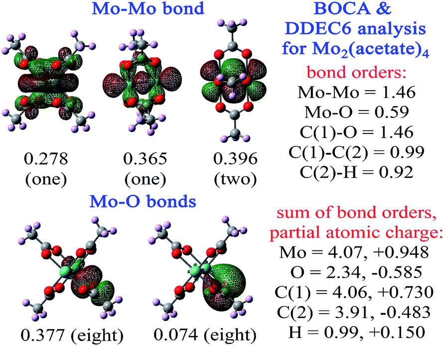 | ||
| Fig. 6 Bond order component analysis for Mo2(acetate)4 using the Pipek–Mezey localized orbitals of the B3LYP/def2tzvppd electron density matrix. The corresponding bond order component per orbital is listed. For each orbital, the total number of analogous orbitals is shown in parentheses. For each displayed Mo–O bonding orbital, the eight analogous orbitals correspond to one per oxygen atom. There are four Mo–Mo bonding orbitals. The two 1πu orbitals (top right panel) are rotated 90° relative to each other. The right column lists computed partial atomic charges, SBOs, and selected bond orders. | ||
Our final example compares the ClO− anion to neutral ClO. As shown in Table 2, ClO− has a relatively high DDEC6 BO of 1.74 compared to its heuristic BO of 1. In contrast, ClO has a DDEC6 BO of 1.647 which is closer to its heuristic BO of 1½. Density and geometry based descriptors are now considered. First, the computed bond lengths are 1.667 (ClO−) and 1.563 (ClO) Å. Second, the DDEC6 〈r3〉 moments of atoms were 84.03 (Cl) and 36.02 (O) bohr3 in ClO− compared to 60.71 (Cl) and 22.99 (O) in ClO, which clearly shows more diffuse atoms in the anion. Third, the electron density at the bond critical point (computed using Multiwfn) was 20.2% lower for ClO− compared to ClO. Fourth, the DDEC6 overlap population (contact exchange) was 5.3% (6.2%) higher for ClO− compared to ClO. Taken together, these results show that ClO− has a longer bond length and lower bond critical point density than neutral ClO, but the increased diffuseness of atoms in ClO− causes larger atomic overlap, contact exchange, and DDEC6 BO compared to ClO. DDEC6 partitioning was reliable for both ClO− and ClO, as evidenced by the modest magnitudes of the atomic dipole moments (≤0.36 atomic units) and atomic quadrupole traceless tensor eigenvalues (≤0.54 atomic units). The molecular dipole magnitudes (in atomic units) based on the NACs were 1.19 (ClO−) and 0.47 (ClO) compared to 0.97 (ClO−) and 0.49 (ClO) from the electron density grid.
We now compare orbital-based descriptors for the ClO− anion to neutral ClO. Fig. 7 illustrates the NSOs and BOCA for ClO and ClO−. It is readily apparent that each σ-orbital and π-orbital is lopsided, with larger lobe size and more electron density concentrated on one of the two atoms. The occupied spin-up and unoccupied spin-down 1πg,x orbitals in ClO provide a natural experiment. In the occupied spin-up 1πg,x orbital, the lobe on the Cl atom is large while the lobe on the O atom is small. This minimizes the kinetic energy, because the larger Cl atom size provides a large lobe diameter. Orthogonality between the 1πg,x and 1πu,x spin-up orbitals then requires that the 1πu,x spin-up orbital is pear-shaped with the larger end on the O atom than on the Cl atom. Because the 1πg,x spin-down orbital is unoccupied, the kinetic energy is minimized by making the 1πu,x spin-down orbital pear-shaped with the larger end on the Cl atom. Hence, kinetic energy factors cause the pear-shaped 1πu,x to flip over between the spin-up and spin-down orbitals. In the ClO− anion, both the spin-up and spin-down 1πg,x orbitals are occupied. Hence, in ClO− the 1πg,x orbital has a larger lobe on the Cl atom, while the pear-shaped 1πu,x orbital has the larger end on the O atom. Hence the occupied spin-down 1πu,x orbital flips over (aka ‘shape-shifts’) between ClO and ClO−. This effect plus the more diffuse orbitals contributes to the high Manz BO in ClO−. As shown in Fig. 7, the 2σg orbital has the highest BOC in both ClO and ClO−. In ClO but not ClO−, the 1πu,x spin-down orbital also has a large BOC. All other orbitals have small BOCs.
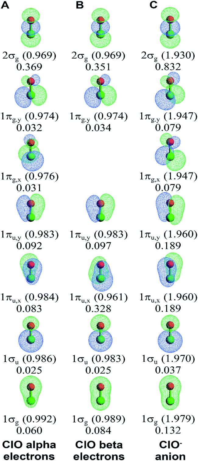 | ||
| Fig. 7 Bond order component analysis (BOCA) for the ClO (doublet) molecule and ClO− (singlet) anion using the natural spin-orbitals. Orbital occupancies are given in parentheses. Bond order components are listed without parentheses. The oxygen atom is displayed in red, while the chlorine atom is displayed in green. | ||
Finally, Table 7 summarizes the computed BOCA parameters κ and η for several materials. As shown in eqn (5), 0 ≤ κ ≤ 1 scales the orbital exchange interference term, while 0 ≤ η ≤ 2 scales the exchange non-interference term. From eqn (16) and (17), η can be non-zero only when κ reaches the upper or lower bound: η = 0 if 0 < κ < 1. For highly stretched bonds between adjacent atoms, one would normally expect κ ≪ 1 due to the small density overlaps between atoms. For highly compressed bonds between adjacent atoms, one would normally expect η > 1 due to the large density overlaps between atoms. Near the equilibrium bond length, one would normally expect κ ≈ 1 and η ≈ 0 between adjacent atoms, except when additional factors come into play.
| κ | η | κ | η | ||
|---|---|---|---|---|---|
| H2+ | 0.60 | 0.00 | Ca2 | 0.86 | 0.00 |
| H2 | 0.96 | 0.00 | Cr2 | 0.67 | 0.00 |
| Li2 | 0.96 | 0.00 | Ge2 | 0.80 | 0.00 |
| Be2 | 0.81 | 0.00 | As2 | 0.79 | 0.00 |
| B2 | 0.84 | 0.00 | Mo2 | 0.71 | 0.00 |
| C2 | 0.88 | 0.00 | Sb2 | 0.73 | 0.00 |
| N2 | 0.99 | 0.00 | ClO | 0.91 | 0.00 |
| O2 | 0.88 | 0.00 | ClO− | 1.00 | 0.15 |
| F2 | 0.79 | 0.00 | Mo2(acetate)4 | 0.45 (Mo–Mo) | 0.00 |
| Ne2 | 1.00 | 0.03 | 1.00 (Mo–O) | 0.00 |
Table 7 highlights six such additional factors. First, Ne2 is bonded primarily by London dispersion interactions producing a η value slightly greater than zero. Second, orbital shape-shifting and diffuseness leads to a relatively high DDEC6 BO in ClO− which produces η slightly greater than zero. Third, the reduced LSCFs of 1σg and 2σg orbitals in Mo2 and Cr2 leads to κ ≈ ⅔ in these compounds. Fourth, electrostatic repulsion between the two atoms produces κ substantially less than 1 in H2+. Fifth, diffuse semi-core electrons in multiple order bonds can lead to decreased κ (e.g., κ = 0.73 for Sb2 with BO = 2.124). Sixth, DFT (at zero temperature) yields an idempotent density matrix that forces electrons to fully occupy the lowest energy orbitals, but correlated wavefunction methods exhibit partial occupancy of the excitation orbitals. Since excitation orbitals are collectively more anti-bonding, this often requires a smaller κ for DFT orbitals than for correlated wavefunction NSOs to produce the same BO. For example, the DFT orbitals of Mo2(acetate)4 have κ = 0.45 for the Mo–Mo bond.
3 Conclusions
Bond order is a fundamental chemical concept that quantifies the number of electrons dressed-exchanged between two atoms in a material.2 Because diatomics are the smallest chemical systems possessing a chemical bond, they have foundational importance to chemistry education pertaining to bond orders. In spite of this fundamental importance, there have been no prior systematic studies of accurate quantum-mechanically calculated bond orders across a large number of diatomics. In this article, we computed bond orders for 288 diatomics including 65 homodiatomic molecules, 217 heterodiatomic molecules, and 6 diatomic ions. We showed bond order is strongly correlated to bond energy within the same chemical group but not necessarily between different chemical groups. For halogens, we showed the large increase in bond order and bond energy from F2 to Cl2 is due to exchange polarization in Cl2. We discussed ways semi-core electrons affect bond orders across the periodic table: (a) electrostatic screening, (b) inaugural subshell effect, and (c) dressed-exchange hole localization. We correlated semi-core electron diffuseness to bond order weakening down various chemical groups.We introduced a bond order component analysis (BOCA) that assigns bond order components to spin-orbitals. This BOCA is derived from first-principles and works for any spin-orbitals that are a unitary transformation of the natural spin-orbitals. This provides a significant advance by showing how to assign bond order components to spin-orbitals in such a way that any choice of spin-orbitals always reproduces the same bond orders. These bond orders are a functional of the electron density and spin magnetization distributions providing consistency across different quantum chemistry methods.2 This BOCA provides chemical insights by showing how different orbitals and orbital symmetry groups (e.g., σg, σu, πg, πu, δg, δu) contribute to the bond order between two atoms in a material. As examples, we presented detailed BOCA for all period 2 homodiatomics, plus Mo2, Cr2, ClO, ClO−, and Mo2(acetate)4. Using these examples, we demonstrated important bond order concepts related to the Virial equilibrium between kinetic and potential energy: (a) bond orders are caused by kinetic energy scaled electron exchange (aka dressed exchange) between atoms in a material, (b) the bond order can be much less than the number of bonding orbitals when in-phase orbital overlaps are only partially effective (e.g., C2, Mo2, and Mo2(acetate)4), and (b) orbital shape-shifting can minimize kinetic energy (e.g., π-orbitals in ClO and ClO−).
We also introduced heuristic models as learning tools. First, we introduced an analogy between passing messages in a computer network and exchanging electrons in a material. The bond order (i.e., number of electrons dressed-exchanged) is analogous to the number of messages being concurrently passed between two computers in the network. A spin-orbital in a material is analogous to a channel in the network. We proposed the bonding versus anti-bonding characteristic describes the difference in overall performance between two states, while bond order components quantify the particular division of message transmission across channels within one state. A spin-orbital is anti-bonding if occupying it decreases the overall bond order, which is analogous to a channel being anti-bonding if adding it to the computer network decreases overall message transmission in the network.
Second, we introduced heuristic molecular orbitals and their associated bond orders and bond order components for all period 2 homodiatomics. The four σ orbitals had substantial s–p mixing whose magnitude was estimated. Most interestingly, the heuristic bond orders were ¾ for Be2, 1¾ for B2, and 2¾ for C2, which confirms these bond orders are non-integer. Heuristic BOCA used these heuristic molecular orbitals and heuristic bond orders as inputs. As summarized in Table 6, there is good agreement between bond order components for σg, σu, πu, and πg orbital symmetry groups for this heuristic model compared to the high-level quantum chemistry calculations. Our computed carbon dimer BOs of 2.73 (eqn (2)), 2.65 (bond length interpolation from Introduction above), and 2¾ (heuristic model) are consistent. This clearly demonstrates that bond orders are finally understood for all period 2 homodiatomics, including Be2, B2, and C2 for which there was much previous disagreement.
4 Methods
4.1 Study design
The molecules selected were: (1) all main group homodiatomics for periods 1–6, (2) transition metal (d-block) homodiatomics for periods 4–6 for which we found literature-reported experimental spin states or bond lengths, (3) heterodiatomics that have spectroscopic constants and dissociation energies available in CRC Handbook of Chemistry and Physics 97th edition,28 and (4) selected ions (H2+, HO−, CN−, CN+, BC−, ClO−). Where available, experimental spin states were used for calculations. For molecules and ions without available experimental spin states, we performed calculations using multiple spin states to identify the lowest-energy spin state.The quantum calculation methods used in this study were coupled-cluster singles doubles (CCSD), symmetry adapted cluster configuration interaction (SAC-CI), and complete active space self-consistent field (CAS-SCF). These methods include electron correlations without empirical parameterization. The CCSD(full) method included single and double excitations of all electrons (except relativistic effective core potential in basis set) from a single reference state.70 The SAC-CI method included single, double, and unlinked quadruple excitations (i.e., products of double excitations) of valence electrons from a symmetry adapted minimal multi-reference spin state.71,72 The CAS-SCF method is a multi-reference configuration interaction method including all excitations within an active space.73 Due to high computational cost of CAS-SCF, it was only feasible to include up to around 16 valence orbitals in the active space. CAS-SCF was used for B2, C2, BN (both singlet and triplet states), CN+ and BC−, which required multi-reference wavefunctions.16,23,30 B2 used 8 doubly-occupied orbitals in the active space; all others used 16 doubly-occupied orbitals in the active space. SAC-CI was used for the weakly binding elements having filled subshells but not filled shells (i.e., groups 2 and 12 homodiatomics), because CCSD was not sufficiently accurate (i.e., bond length errors >10%) and SAC-CI allowed more orbitals to be correlated than the more expensive CAS-SCF. The weakly binding Mn2 (half-filled d-subshell) used SAC-CI because CCSD did not converge and CAS-SCF was too expensive. For the weakly bound XeF spin doublet, a CCSD(full) electron density was generated at the SAC-CI optimized geometry (which was nearly identical to the experimental geometry), because CCSD and CAS-SCF (15 electrons in 13 alpha orbitals and 13 beta orbitals) yielded bond length errors >30% and wfx file generation was not available using the SAC-CI spin doublet electron density. Everything else used CCSD(full). Wavefunctions and bond orders for 25 diatomics (which also used these same methods) were from Manz's prior study.2
Manz's method to compute bond orders was used, because it accurately computes bond orders as a functional of the electron and spin density distributions.2 This makes the bond orders consistent across different quantum chemistry methods (i.e., exchange–correlation theories and basis sets).2 It is derived from first-principles and applies to a wide range of materials and bonding types.2
4.2 Quantum calculation methods
We performed the quantum chemistry calculations using the Gaussian16 program.74 To ensure the calculation results are meaningful, we optimized the bond length in Gaussian16 and compared the optimized bond length to the experimental data. The geometry optimization convergence criteria were root-mean squared (RMS) force is less than 0.0003 Hartrees per bohr and RMS displacement is less than 0.0012 Bohr. Since the geometry optimization of Mn2 did not numerically converge (due to software issues), we used the experimental bond length of 3.4 Å (ref. 75) for this molecule.We used the def2QZVPPD basis set76 downloaded from the EMSL basis set exchange.77 This is a quadruple zeta basis set with two polarization and one diffuse functions. This basis set uses RECPs for Rb (element 37) and heavier elements. The number of electrons included in the RECPs is 28 for elements 37–54, 46 for elements 55–57, and 60 for elements 72–86. Since SAC-CI calculations using def2QZVPPD did not converge for Ca2, Sr2, and Ba2, the def2TZVPPD basis set76 was used for these molecules. For W2, our CCSD calculations did not converge with either of these two basis sets, so we used the SDD basis set from the EMSL basis set exchange having a RECP replacing 60 core electrons.77,78 All properties, including the correlated relaxed electron density, were computed using the same basis set and exchange–correlation theory (except for XeF as noted above) as used to optimize the molecular geometry.
For each molecule computed via the SAC-CI method, a preliminary (‘level one’) calculation computed energies across eight different symmetry states to identify the low-energy symmetry state. SAC-CI geometry optimization was subsequently performed in Gaussian16 using the accurate default cutoffs (‘level three’), with the target state set to the appropriate low-energy symmetry. Three macro iterations were performed to ensure self-consistent orbital selection during geometry optimization.79
4.3 Bond analysis methods
Natural spin-orbitals (NSOs) were computed in Gaussian16 and saved to wfx files. This generated separate alpha NSOs and beta NSOs by diagonalizing the correlated relaxed electron density matrices for spin-up and spin-down electrons, respectively. These wfx files contained the fractional orbital occupancies associated with the correlated wavefunction. The NSOs displayed in Fig. 2, 4, and 7 were generated in the Multiwfn80 program by reading the wfx files.The semi-core density analysis summarized in Fig. 3 proceeded as follows. First, wfx files were prepared containing all the core electrons (including semi-core electrons) without valence electrons. Second, these wfx files were read into the Multiwfn program and the electron density at evenly spaced points along the axis joining the two nuclei was printed to a file. We analyzed data in this file to find the distances d−1, d−2, d−3, and the associated percentages listed in Fig. 3C.
Wiberg bond indices (WBI) in the natural atomic orbital (NAO) basis were computed using the NBO program with bond resonance enabled. As shown in Table S1 of ESI,† results for NBO version 3.1 (built into Gaussian software) were compared to those from NBO version 6.0 (ref. 53 and 81) (standalone program). Because the NAO's are orthonormal, the WBI in the NAO basis equals the Mayer bond index3 (MBI) in the NAO basis.
DDEC6 bond orders were computed using the Chargemol5 program. In the Chargemol program, Manz's bond order equations can be used with different charge partitioning schemes (e.g., DDEC6 or DDEC3).5 We used DDEC6 charge partitioning,7 because this provides reliable results across a wide range of material types.2,6,7 This method assigns atomic electron density distributions that simultaneously resemble their spherical averages and charge-compensated reference ions, using constraints to ensure the atomic electron density tails are not too diffuse or too contracted.7 All density derived electrostatic and chemical (DDEC) methods use the spin partitioning method of Manz and Sholl.5,82 This method assigns atomic spin magnetization density distributions that simultaneously resemble their spherical averages and proportional spin partitions,82 which is important to satisfy the confluence of atomic exchange propensities.2 Integration grids for charge partitioning, spin partitioning, and bond order analysis were the same as used in prior studies.2,5–7,83 A 5 Å cutoff radius around each atom was used for integrations.2,5–7,83
BOCA was programmed into the Chargemol program. The AOMs were integrated using atom-centered grids with integration points in the spherical coordinates (rA, θA, ϕA) for each atom A over the ranges 0 ≤ rA ≤ 5 Å, 0 ≤ θA ≤ π, 0 ≤ ϕA < 2π. Many suitable atom-centered integration grids of this type have been described in prior literature.84–88
For Mo2(acetate)4, the Pipek–Mezey89 localized orbitals were generated in Gaussian16 and saved to a fchk file. Multiwfn read this fchk file and saved the Pipek–Mezey orbitals to a wfx file. (This procedure was required, because Gaussian16 is not currently set up to save the Pipek–Mezey localized orbitals to a wfx file.) All other wfx files were saved directly from Gaussian software as described above. The Chargemol program read in these wfx files and performed DDEC6 analysis and BOCA.
4.4 Statistical analysis
This computational approach was validated by comparing optimized to experimental (where available) bond lengths. Fig. 8 compares optimized to experimental bond lengths for both homodiatomics and heterodiatomics. The mean relative errors (MRE) and mean absolute relative errors (MARE) between calculated and experimental bond lengths were: (a) MRE = 0.13%, MARE = 2.39%, and st. dev. = 3.38% for homodiatomics and (b) MRE = −0.16%, MARE = 0.84%, and st. dev. = 1.14% for heterodiatomics. For homodiatomics (Table S2 of ESI†) and heterodiatomics (Table S3 of ESI†), all computed bond lengths were within ±10% of experimental values.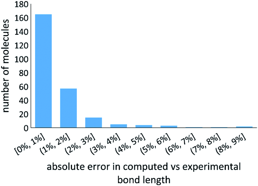 | ||
| Fig. 8 Histogram for the bond length error. This plot includes all the homodiatomics and heterodiatomics for which reference experimental bond lengths are listed. | ||
Funding
NSF CAREER award DMR-1555376 provided financial support. The Extreme Science and Engineering Discovery Environment90 (NSF ACI-1548562) project TG-CTS100027 provided computational time on the Comet cluster at the San Diego Supercomputing Center and the Stampede2 cluster at the Texas Advanced Computing Center.Authors' contributions
T. C. performed the majority of the quantum chemistry calculations with some performed by T. A. M. T. A. M. conceived and supervised the study and came up with all of the new mathematical equations, mathematical proofs, methods, heuristic model, network analogy, and programmed BOCA into Chargemol. Both authors analyzed data and wrote the manuscript.Conflicts of interest
There are no conflicts to declare.References
- G. N. Lewis, The atom and the molecule, J. Am. Chem. Soc., 1916, 38, 762–785, DOI:10.1021/ja02261a002.
- T. A. Manz, Introducing DDEC6 atomic population analysis: part 3. Comprehensive method to compute bond orders, RSC Adv., 2017, 7, 45552–45581, 10.1039/c7ra07400j.
- I. Mayer, On bond orders and valences in the abinitio quantum chemical theory, Int. J. Quantum Chem., 1986, 29, 73–84, DOI:10.1002/qua.560290108.
- A. J. Coleman, Structure of fermion density matrices, Rev. Mod. Phys., 1963, 35, 668–687, DOI:10.1103/RevModPhys.35.668.
- N. Gabaldon Limas and T. A. Manz, Introducing DDEC6 atomic population analysis: part 4. Efficient parallel computation of net atomic charges, atomic spin moments, bond orders, and more, RSC Adv., 2018, 8, 2678–2707, 10.1039/c7ra11829e.
- N. Gabaldon Limas and T. A. Manz, Introducing DDEC6 atomic population analysis: part 2. Computed results for a wide range of periodic and nonperiodic materials, RSC Adv., 2016, 6, 45727–45747, 10.1039/c6ra05507a.
- T. A. Manz and N. Gabaldon Limas, Introducing DDEC6 atomic population analysis: part 1. Charge partitioning theory and methodology, RSC Adv., 2016, 6, 47771–47801, 10.1039/c6ra04656h.
- P. Politzer, Bond orders of heteronuclear diatomic molecules, J. Chem. Phys., 1969, 51, 459–460, DOI:10.1063/1.1671755.
- P. Politzer, Bond orders of homonuclear diatomic molecules, J. Chem. Phys., 1969, 50, 2780–2781, DOI:10.1063/1.1671457.
- B. O. Roos, A. C. Borin and L. Gagliardi, Reaching the maximum multiplicity of the covalent chemical bond, Angew. Chem., Int. Ed., 2007, 46, 1469–1472, DOI:10.1002/anie.200603600.
- E. Matito, M. Sola, P. Salvador and M. Duran, Electron sharing indexes at the correlated level. Application to aromaticity calculations, Faraday Discuss., 2007, 135, 325–345, 10.1039/b605086g.
- R. J. Wheatley and A. A. Gopal, Covalent bond orders and atomic anisotropies from iterated stockholder atoms, Phys. Chem. Chem. Phys., 2012, 14, 2087–2091, 10.1039/c2cp23504h.
- I. Mayer, Bond order and valence indices: a personal account, J. Comput. Chem., 2007, 28, 204–221, DOI:10.1002/jcc.20494.
- D. Vanfleteren, D. Van Neck, P. Bultinck, P. W. Ayers and M. Waroquier, Stockholder projector analysis: a Hilbert-space partitioning of the molecular one-electron density matrix with orthogonal projectors, J. Chem. Phys., 2012, 136, 014107, DOI:10.1063/1.3673321.
- R. L. Dekock and H. B. Gray, Chemical Structure and Bonding, University Science Books, Sausalito, California, 2nd edn, 1989, ISBN: 978-0935702613 Search PubMed.
- M. Hermann and G. Frenking, The chemical bond in C2, Chem.–Eur. J., 2016, 22, 4100–4108, DOI:10.1002/chem.201503762.
- L. T. Xu and T. H. Dunning, Insights into the perplexing nature of the bonding in C2 from generalized valence bond calculations, J. Chem. Theory Comput., 2014, 10, 195–201, DOI:10.1021/ct400867h.
- J. Grunenberg, Comment on “The nature of the fourth bond in the ground state of C2: The quadruple bond conundrum”, Chem.–Eur. J., 2015, 21, 17126, DOI:10.1002/chem.201500130.
- D. L. Cooper, F. E. Penotti and R. Ponec, Why is the bond multiplicity in C2 so elusive?, Comput. Theor. Chem., 2015, 1053, 189–194, DOI:10.1016/j.comptc.2014.08.024.
- D. de Sousa and M. Nascimento, Is there a quadruple bond in C2?, J. Chem. Theory Comput., 2016, 12, 2234–2241, DOI:10.1021/acs.jctc.6b00055.
- A. Forni and M. Sironi, The nature of the carbon-carbon bond in the C2 and C2H2 molecules, Theor. Chim. Acta, 1995, 92, 49–59, DOI:10.1007/bf01134203.
- D. L. Cooper, R. Ponec and M. Kohout, New insights from domain-averaged Fermi holes and bond order analysis into the bonding conundrum in C2, Mol. Phys., 2016, 114, 1270–1284, DOI:10.1080/00268976.2015.1112925.
- S. Shaik, D. Danovich, W. Wu, P. F. Su, H. S. Rzepa and P. C. Hiberty, Quadruple bonding in C2 and analogous eight-valence electron species, Nat. Chem., 2012, 4, 195–200, DOI:10.1038/nchem.1263.
- S. Shaik, H. S. Rzepa and R. Hoffmann, One molecule, two atoms, three views, four bonds?, Angew. Chem., Int. Ed., 2013, 52, 3020–3033, DOI:10.1002/anie.201208206.
- S. Shaik, D. Danovich, B. Braida and P. C. Hiberty, The quadruple bonding in C2 reproduces the properties of the molecule, Chem.–Eur. J., 2016, 22, 4116–4128, DOI:10.1002/chem.201600011.
- J. M. Matxain, F. Ruiperez, I. Infante, X. Lopez, J. M. Ugalde, G. Merino and M. Piris, Communication: Chemical bonding in carbon dimer isovalent series from the natural orbital functional theory perspective, J. Chem. Phys., 2013, 138, 151102, DOI:10.1063/1.4802585.
- R. L. Zhong, M. Zhang, H. L. Xu and Z. M. Su, Latent harmony in dicarbon between VB and MO theories through orthogonal hybridization of 3σg and 2σu, Chem. Sci., 2016, 7, 1028–1032, 10.1039/c5sc03437j.
- CRC Handbook of Chemistry and Physics, ed. W. M. Haynes, CRC Press, Boca Raton, FL, 97th edn, 2016–2017, pp. 9.73-9.77, 9.107-9.112. ISBN: 978-1-4987-5428-6 Search PubMed.
- L. Pauling, Atomic radii and interatomic distances in metals, J. Am. Chem. Soc., 1947, 69, 542–553, DOI:10.1021/ja01195a024.
- Z. Rashid, J. H. van Lenthe and R. W. A. Havenith, Bonding in B2 and B2+: Insights from full configuration interaction and valence bond studies, Comput. Theor. Chem., 2017, 1116, 92–95, DOI:10.1016/j.comptc.2017.02.001.
- R. Y. Rohling, I. C. Tranca, E. J. M. Hensen and E. A. Pidko, Correlations between density-based bond orders and orbital-based bond energies for chemical bonding analysis, J. Phys. Chem. C, 2019, 123, 2843–2854, DOI:10.1021/acs.jpcc.8b08934.
- O. Mo, M. Yanez, M. Eckert-Maksic, Z. B. Maksic, I. Alkorta and J. Elguero, Periodic trends in bond dissociation energies. A theoretical study, J. Phys. Chem. A, 2005, 109, 4359–4365, DOI:10.1021/jp050857o.
- M. J. Frisch, G. W. Trucks, H. B. Schlegel, G. E. Scuseria, M. A. Robb, J. R. Cheeseman, G. Scalmani, V. Barone, B. Mennucci, G. A. Petersson, H. Nakatsuji, M. Caricato, X. Li, H. P. Hratchian, A. F. Izmaylov, J. Bloino, G. Zheng, J. L. Sonnenberg, M. Hada, M. Ehara, K. Toyota, R. Fukuda, J. Hasegawa, M. Ishida, T. Nakajima, Y. Honda, O. Kitao, H. Nakai, T. Vreven, J. A. J. Montgomery, J. E. Peralta, F. Ogliaro, M. Bearpark, J. J. Heyd, E. Brothers, K. N. Kudin, V. N. Staroverov, T. Keith, R. Kobayashi, J. Normand, K. Raghavachari, A. Rendell, J. C. Burant, S. S. Iyengar, J. Tomasi, M. Cossi, N. Rega, J. M. Millam, M. Klene, J. E. Knox, J. B. Cross, V. Bakken, C. Adamo, J. Jaramillo, R. Gomperts, R. E. Stratmann, O. Yazyev, A. J. Austin, R. Cammi, C. Pomelli, J. W. Ochterski, R. L. Martin, K. Morokuma, V. G. Zakrzewski, G. A. Voth, P. Salvador, J. J. Dannenberg, S. Dapprich, A. D. Daniels, O. Farkas, J. B. Foresman, J. V. Ortiz, J. Cioslowski and D. J. Fox, Gaussian 09 software program, Gaussian Inc., Wallingford, CT, 2009 Search PubMed.
- T. Nakajima and K. Hirao, The Douglas-Kroll-Hess approach, Chem. Rev., 2012, 112, 385–402, DOI:10.1021/cr200040s.
- L. Visscher and K. G. Dyall, Dirac-Fock atomic electronic structure calculations using different nuclear charge distributions, At. Data Nucl. Data Tables, 1997, 67, 207–224, DOI:10.1006/adnd.1997.0751.
- J. P. Perdew, K. Burke and M. Ernzerhof, Generalized gradient approximation made simple, Phys. Rev. Lett., 1996, 77, 3865–3868, DOI:10.1103/PhysRevLett.77.3865.
- T. A. Manz and D. S. Sholl, Chemically meaningful atomic charges that reproduce the electrostatic potential in periodic and nonperiodic materials, J. Chem. Theory Comput., 2010, 6, 2455–2468, DOI:10.1021/ct100125x.
- L. Pauling, The nature of the chemical bond. Application of results obtained from the quantum mechanics and from a theory of paramagnetic susceptibility to the structure of molecules, J. Am. Chem. Soc., 1931, 53, 1367–1400, DOI:10.1021/ja01355a027.
- R. Hoffmann and R. Woodward, Conservation of orbital symmetry, Acc. Chem. Res., 1968, 1, 17–22, DOI:10.1021/ar50001a003.
- S. Lehtola and H. Jonsson, Unitary optimization of localized molecular orbitals, J. Chem. Theory Comput., 2013, 9, 5365–5372, DOI:10.1021/ct400793q.
- S. Lehtola and H. Jonsson, Pipek-Mezey orbital localization using various partial charge estimates, J. Chem. Theory Comput., 2014, 10, 642–649, DOI:10.1021/ct401016x.
- E. O. Jonsson, S. Lehtola, M. Puska and H. Jonsson, Theory and applications of generalized Pipek-Mezey Wannier functions, J. Chem. Theory Comput., 2017, 13, 460–474, DOI:10.1021/acs.jctc.6b00809.
- Y. L. Wang, H. S. Hu, W. L. Li, F. Wei and J. Li, Relativistic effects break periodicity in Group 6 diatomic molecules, J. Am. Chem. Soc., 2016, 138, 1126–1129, DOI:10.1021/jacs.5b11793.
- C. Benelli and D. Gatteschi, Introduction to Molecular Magnetism: From Transition Metals to Lanthanides, Wiley-VCH, Weinheim, Germany, 2015, ISBN: 978-3-527-33540-4 Search PubMed.
- H. P. Wijn, Magnetic Properties of Metals, Springer-Verlag, Berlin, Germany, 1991, ISBN: 978-3-540-53485-3 Search PubMed.
- W. Kutzelnigg, Chemical bonding in higher main group elements, Angew. Chem., Int. Ed., 1984, 23, 272–295, DOI:10.1002/anie.198402721.
- P. P. Power, π-bonding and the lone pair effect in multiple bonds between heavier main group elements, Chem. Rev., 1999, 99, 3463–3503, DOI:10.1021/cr9408989.
- M. C. Heaven, V. E. Bondybey, J. M. Merritt and A. L. Kaledin, The unique bonding characteristics of beryllium and the Group IIA metals, Chem. Phys. Lett., 2011, 506, 1–14, DOI:10.1016/j.cplett.2011.02.025.
- J. M. Merritt, V. E. Bondybey and M. C. Heaven, Beryllium dimer-caught in the act of bonding, Science, 2009, 324, 1548–1551, DOI:10.1126/science.1174326.
- A. Kalemos, The nature of the chemical bond in Be2+, Be2, Be2−, and Be3, J. Chem. Phys., 2016, 145, 214302, DOI:10.1063/1.4967819.
- L. T. Xu and T. H. Dunning, Generalized valence bond description of the ground states (X1Σg+) of homonuclear pnictogen diatomic molecules: N2, P2, and As2, J. Chem. Theory Comput., 2015, 11, 2496–2507, DOI:10.1021/acs.jctc.5b00104.
- K. Ruedenberg and M. W. Schmidt, Physical understanding through variational reasoning: Electron sharing and covalent bonding, J. Phys. Chem. A, 2009, 113, 1954–1968, DOI:10.1021/jp807973x.
- E. D. Glendening, C. R. Landis and F. Weinhold, NBO 6.0: Natural bond orbital analysis program, J. Comput. Chem., 2013, 34, 1429–1437, DOI:10.1002/jcc.23266.
- A. E. Reed, L. A. Curtiss and F. Weinhold, Intermolecular interactions from a natural bond orbital, donor-acceptor viewpoint, Chem. Rev., 1988, 88, 899–926, DOI:10.1021/cr00088a005.
- T. Janowski, Near equivalence of intrinsic atomic orbitals and quasiatomic orbitals, J. Chem. Theory Comput., 2014, 10, 3085–3091, DOI:10.1021/ct500245f.
- A. E. Reed, R. B. Weinstock and F. Weinhold, Natural population analysis, J. Chem. Phys., 1985, 83, 735–746, DOI:10.1063/1.449486.
- P. A. M. Dirac, The quantum theory of the electron, Proc. R. Soc. London, Ser. A, 1928, 117, 610–624, DOI:10.1098/rspa.1928.0023.
- P. O. Lowdin, Scaling problem, virial theorem, and connected relations in quantum mechanics, J. Mol. Spectrosc., 1959, 3, 46–66, DOI:10.1016/0022-2852(59)90006-2.
- J. Erhart, S. Sponar, G. Sulyok, G. Badurek, M. Ozawa and Y. Hasegawa, Experimental demonstration of a universally valid error-disturbance uncertainty relation in spin measurements, Nat. Phys., 2012, 8, 185–189, DOI:10.1038/NPHYS2194.
- K. Ruedenberg, The physical nature of the chemical bond, Rev. Mod. Phys., 1962, 34, 326–376, DOI:10.1103/RevModPhys.34.326.
- K. Ruedenberg and M. W. Schmidt, Why does electron sharing lead to covalent bonding? A variational analysis, J. Comput. Chem., 2007, 28, 391–410, DOI:10.1002/jcc.20553.
- J. G. Angyan, M. Loos and I. Mayer, Covalent bond orders and atomic valence indices in the topological theory of atoms in molecules, J. Phys. Chem., 1994, 98, 5244–5248, DOI:10.1021/j100071a013.
- I. Mayer and P. Salvador, Overlap populations, bond orders and valences for 'fuzzy' atoms, Chem. Phys. Lett., 2004, 383, 368–375, DOI:10.1016/j.cplett.2003.11.048.
- R. F. W. Bader and M. E. Stephens, Spatial localization of the electronic pair and number distribution in molecules, J. Am. Chem. Soc., 1975, 97, 7391–7399, DOI:10.1021/ja00859a001.
- K. Hino, Y. Saito and M. Benard, Electron-density distribution in crystals of tetra-μ-acetato-dimolybdenum(Mo-Mo), Acta Crystallogr., Sect. B: Struct. Sci., 1981, 37, 2164–2170, DOI:10.1107/S0567740881008303.
- J. F. Vandermaelen and J. A. Cabeza, QTAIM analysis of the bonding in Mo-Mo bonded dimolybdenum complexes, Inorg. Chem., 2012, 51, 7384–7391, DOI:10.1021/ic300845g.
- F. A. Cotton, in Multiple Bonds Between Metal Atoms, ed. F. A. Cotton, C. A. Murillo and R. A. Walton, Springer, Boston, MA, 2005, pp. 69–182, ISBN 978-0-387-25829-4 Search PubMed.
- F. A. Cotton and X. J. Feng, Density functional theory study of transition-metal compounds containing metal-metal bonds. 2. Molecular structures and vibrational spectra of dinuclear tetracarboxylate compounds of molybdenum and rhodium, J. Am. Chem. Soc., 1998, 120, 3387–3397, DOI:10.1021/ja9738236.
- F. A. Cotton, Z. C. Mester and T. R. Webb, Dimolybdenum tetraacetate, Acta Crystallogr., Sect. B: Struct. Sci., 1974, 30, 2768–2770, DOI:10.1107/S0567740874008053.
- J. D. Watts, J. Gauss and R. J. Bartlett, Coupled-cluster methods with noniterative triple excitations for restricted open-shell Hartree-Fock and other general single determinant reference functions. Energies and analytical gradients, J. Chem. Phys., 1993, 98, 8718–8733, DOI:10.1063/1.464480.
- H. Nakatsuji, Cluster expansion of the wavefunction. Calculation of electron correlations in ground and excited states by SAC and SAC CI theories, Chem. Phys. Lett., 1979, 67, 334–342, DOI:10.1016/0009-2614(79)85173-8.
- H. Nakatsuji and K. Hirao, Cluster expansion of wavefunction. Symmetry-adapted-cluster expansion, its variational determination, and extension of open-shell orbital theory, J. Chem. Phys., 1978, 68, 2053–2065, DOI:10.1063/1.436028.
- N. Yamamoto, T. Vreven, M. A. Robb, M. J. Frisch and H. B. Schlegel, A direct derivative MC-SCF procedure, Chem. Phys. Lett., 1996, 250, 373–378, DOI:10.1016/0009-2614(96)00027-9.
- M. J. Frisch, G. W. Trucks, H. B. Schlegel, G. E. Scuseria, M. A. Robb, J. R. Cheeseman, G. Scalmani, V. Barone, G. A. Petersson, H. Nakatsuji, X. Li, M. Caricato, A. V. Marenich, J. Bloino, B. G. Janesko, R. Gomperts, B. Mennucci, H. P. Hratchian, J. V. Ortiz, A. F. Izmaylov, J. L. Sonnenberg, D. Williams-Young, F. Ding, F. Lipparini, F. Egidi, J. Goings, B. Peng, A. Petrone, T. Henderson, D. Ranasinghe, V. G. Zakrzewski, J. Gao, N. Rega, G. Zheng, W. Liang, M. Hada, M. Ehara, K. Toyota, R. Fukuda, J. Hasegawa, M. Ishida, T. Nakajima, Y. Honda, O. Kitao, H. Nakai, T. Vreven, K. Throssell, J. A. Montgomery, Jr., J. E. Peralta, F. Ogliaro, M. J. Bearpark, J. J. Heyd, E. N. Brothers, K. N. Kudin, V. N. Staroverov, T. A. Keith, R. Kobayashi, J. Normand, K. Raghavachari, A. P. Rendell, J. C. Burant, S. S. Iyengar, J. Tomasi, M. Cossi, J. M. Millam, M. Klene, C. Adamo, R. Cammi, J. W. Ochterski, R. L. Martin, K. Morokuma, O. Farkas, J. B. Foresman and D. J. Fox, Gaussian 16 software program, Gaussian Inc., Wallingford, CT, 2016 Search PubMed.
- S. Yanagisawa, T. Tsuneda and K. Hirao, Investigation of the use of density functionals in second- and third-row transition metal dimer calculations, J. Chem. Phys., 2000, 112, 545–553, DOI:10.1002/jcc.1148.
- D. Rappoport and F. Furche, Property-optimized Gaussian basis sets for molecular response calculations, J. Chem. Phys., 2010, 133, 134105, DOI:10.1063/1.3484283.
- K. L. Schuchardt, B. T. Didier, T. Elsethagen, L. S. Sun, V. Gurumoorthi, J. Chase, J. Li and T. L. Windus, Basis set exchange: a community database for computational sciences, J. Chem. Inf. Model., 2007, 47, 1045–1052, DOI:10.1021/ci600510j.
- D. Andrae, U. Haussermann, M. Dolg, H. Stoll and H. Preuss, Energy-adjusted ab initio pseudopotentials for the second and third row transition elements, Theor. Chim. Acta, 1990, 77, 123–141, DOI:10.1007/BF01114537.
- H. Nakatsuji, SAC/SAC-CI Program Guide, Kyoto University, Kyota, Japan, 2005 Search PubMed.
- T. Lu and F. W. Chen, Multiwfn: a multifunctional wavefunction analyzer, J. Comput. Chem., 2012, 33, 580–592, DOI:10.1002/jcc.22885.
- E. D. Glendening, J. K. Badenhoop, A. E. Reed, J. E. Carpenter, J. A. Bohmann, C. M. Morales, C. R. Landis and F. Weinhold, NBO 6.0 software program, Theoretical Chemistry Institute, University of Wisconsin, Madison, Wisconsin, 2013 Search PubMed.
- T. A. Manz and D. S. Sholl, Methods for computing accurate atomic spin moments for collinear and noncollinear magnetism in periodic and nonperiodic materials, J. Chem. Theory Comput., 2011, 7, 4146–4164, DOI:10.1021/ct200539n.
- T. A. Manz and D. S. Sholl, Improved atoms-in-molecule charge partitioning functional for simultaneously reproducing the electrostatic potential and chemical states in periodic and nonperiodic materials, J. Chem. Theory Comput., 2012, 8, 2844–2867, DOI:10.1021/ct3002199.
- A. D. Becke, A multicenter numerical integration scheme for polyatomic molecules, J. Chem. Phys., 1988, 88, 2547–2553, DOI:10.1063/1.454033.
- C. W. Murray, N. C. Handy and G. J. Laming, Quadrature schemes for integrals of density functional theory, Mol. Phys., 1993, 78, 997–1014, DOI:10.1080/00268979300100651.
- R. Lindh, P. A. Malmqvist and L. Gagliardi, Molecular integrals by numerical quadrature. I. Radial integration, Theor. Chem. Acc., 2001, 106, 178–187, DOI:10.1007/s002140100.
- O. Treutler and R. Ahlrichs, Efficient molecular numerical integration schemes, J. Chem. Phys., 1995, 102, 346–354, DOI:10.1063/1.469408.
- P. M. W. Gill, B. G. Johnson and J. A. Pople, A standard grid for density functional calculations, Chem. Phys. Lett., 1993, 209, 506–512, DOI:10.1016/0009-2614(93)80125-9.
- J. Pipek and P. G. Mezey, A fast intrinsic localization procedure applicable for ab initio and semiempirical linear combination of atomic orbital wave functions, J. Chem. Phys., 1989, 90, 4916–4926, DOI:10.1063/1.456588.
- J. Towns, T. Cockerill, M. Dahan, I. Foster, K. Gaither, A. Grimshaw, V. Hazlewood, S. Lathrop, D. Lifka, G. D. Peterson, R. Roskies, J. R. Scott and N. Wilkins-Diehr, XSEDE: accelerating scientific discovery, Comput. Sci. Eng., 2014, 16, 62–74, DOI:10.1109/MCSE.2014.80.
Footnote |
| † Electronic supplementary information (ESI) available: A pdf file containing: mathematical derivations of the BOCA equations; Table S1 comparing bond orders for singlet states of C2, BN, CN+, CB− at different levels of theory; Table S2 listing data for homodiatomic molecules; Table S3 listing data for heterodiatomic molecules; Table S4 listing optimized bond lengths and bond orders for Tl2, Pb2, Bi2, Po2, At2, and Rn2 using all-electron fourth-order relativistic calculations with spin–orbit coupling; Table S5 listing high-level quantum-mechanically computed BOCA results for period 2 homodiatomics. See DOI: 10.1039/c9ra00974d |
| This journal is © The Royal Society of Chemistry 2019 |