
 Open Access Article
 This Open Access Article is licensed under a Creative Commons Attribution-Non Commercial 3.0 Unported Licence
Helically-driven granular mobility and gravity-variant scaling relations†
Andrew Thoesen ,
Teresa McBryan and
Hamidreza Marvi*
,
Teresa McBryan and
Hamidreza Marvi*
School for Engineering of Matter, Transport and Energy (SEMTE), Arizona State University, Tempe, Arizona, USA. E-mail: hmarvi@asu.edu
First published on 23rd April 2019
Abstract
This study discusses the role and function of helical design as it relates to slippage during translation of a vehicle in glass bead media. We show discrete element method (DEM) and multi-body dynamics (MBD) simulations and experiments of a double-helix Archimedes screw propelled vehicle traveling in a bed of soda-lime glass beads. Utilizing granular parameters from the literature and a reduced Young's modulus, we validate the set of granular parameters against experiments. The results suggest that MBD-DEM provides reliable dynamic velocity estimates. We provide the glass, ABS, and glass–ABS simulation parameters used to obtain these results. We also examine recently developed granular scaling laws for wheels applied to these shear-driven vehicles under three different simulated gravities. The results indicate that the system obeys gravity granular scaling laws for constant slip conditions but is limited in each gravity regime when slip begins to increase.
1 Introduction
Vehicles traverse granular media through complex reactions with large numbers of small particles. Much of the research around this focuses on wheeled surface vehicles reacting under primarily normal pressures. There is a long-standing interest to better understand mobility in granular environments within both the robotics and granular physics communities.1–9 This is important for new mobility and material transfer solutions, particularly in the space sector where increased mass and volume are often costly while increased moving parts or complexity are regarded as increasing risk. This complexity is further compounded by the variety of granular materials which exist. There are many approaches to addressing these challenges.10 However, characteristics such as particle size, angularity, and homogeneity of mixture can result in limited applicability of empirical laws or DEM simulations and may require fitting parameters derived from lengthy complimentary tests or other limitations. Here we evaluate a simulation method to replicate dynamic movement and experimental results of a screw-driven craft. This set of observations is broadened to include recently developed granular scaling laws in simulated environments of reduced gravity.Screw-propelled vehicles (SPV's) have been investigated for use on Earth in unstable or uncertain environments for many years. One early example of SPV's was the Marsh Screw Amphibian.11 This craft propelled itself through water and then quickly transitioned to a muddy environment. Another similar vehicle is the Amphirol.12 This vehicle is capable of navigating through sticky wet clay, a nearly impossible task for other forms of transportation including treaded vehicles. The Arctic has also been a tested environment where SPV's show utility, such as the ZIL-2906 (ref. 13) craft used for rescuing cosmonauts. DEM co-simulations have been used in various ways to address granular vehicle mobility, including tire-tread interactions,14 but experimental and DEM simulation studies which characterize dynamics for screws are notably absent. By utilizing a helical piece of rotating geometry, the MBD-DEM simulations and granular scaling laws are tested by a more complex set of shear and normal forces.
In recent years, advancements in computational power have led to varied simulation approaches. Discrete element method (DEM) simulation is an emerging approach whereby each individual particle is modeled as to affect the other particles in a granular media. It can be used for evaluating the terramechanics of a craft in granular media, including in varied gravity.15 Other uses of DEM include testing deformable materials,16–18 evaluating the dynamics of additive manufacturing19,20 and particle beds,21 or assessing the physical properties of a new material.22 It has also been used to analyze jamming/packing problems23,24 or evaluate granular properties of shapes.25 In one case, it was used for both, showing that helical textures on the inside of pipes transporting granular media help evenly distribute mass flow and prevent jamming events.26 Another simulation type, multi-body dynamics (MBD), evaluates the solid bodies or links of a dynamic system and the joints that restrict their relative motion, and how they react to internal and external forces. It can provide tools to study systems which are too large to test,27 have conditions that would be difficult to replicate,28 or would be prohibitively expensive to pursue initial prototypes. DEM has also been combined with other methods such as finite element modeling (FEM) to evaluate deformation in shot-peening29 or powder compaction.30 In our study, DEM and MBD have been co-simulated to replicate both granular and craft dynamics. Validating such results in Earth gravity can provide better insight to reduced gravity simulations. Techniques such as weight-offset on Earth do not take the difference of gravitational compaction of grains into account31,32 and can have erroneous, sometimes opposite trends to actual gravity reduction. Since parabolic flights are often expensive and inaccessible, MBD-DEM co-simulation provides an opportunity for designing and testing robotic craft for space. Coupling between DEM and MBD software can prove difficult33 and an essential part of advancing the simulation community is experimental validation and comparison with reliable real-world counterparts.34–38
There have also been efforts to understand granular dynamics and craft motion from a more theoretical point of view. Granular resistive force theory (RFT), for example, is based on generalized empirical insights and superposition. Scientist can discretize intruders into a collection of smaller structures and sum the resultant forces for analysis under certain conditions.39–43 This has been validated for uniform-thickness intruders under certain assumptions. Modeling granular media as a continuum has received focus in recent years.7,44,45 This includes the emergence of generalized scaling laws which have been successfully tested and verified experimentally. These scaling laws also successfully predicted the DEM simulations results of gravity variation on arbitrarily shaped wheels.46 We evaluate a gravity-variant subset of these laws with our helical geometry and examine whether the craft adheres to such scaling.
In this study, we first examine if a well-characterized media can be replicated in MBD-DEM co-simulations successfully for a dynamic craft. Section 2 introduces the methods of experimentation and simulation models. These results are then analyzed and compared in Section 3 to determine the predictive power of DEM for this scenario. We also introduce non-Earth gravity simulations. This leads to a discussion in Section 4 of the utility of DEM simulations for estimating complex intruder speed as well as comparisons to recently developed granular scaling laws in varied levels of gravity. Finally, in Section 5 we explore future paths for developing capabilities to model granular media for complex intruder design in both Earth and space applications.
2 Methods
2.1 Laboratory experiments
Three screws with dimensions of 10 cm axial length by 5 cm diameter were created in Solidworks and printed using Acrylonitrile Butadiene Styrene (ABS) on a Stratasys 3D printing system. Pitch lengths of 4 cm, 6 cm, and 8 cm were used. This translates to helix angles of 75.7°, 69.1°, and 63° respectively. The versions of the craft using these pitch lengths will be referred to as “P4”, “P6”, and “P8”. The body of the craft was similarly printed and contains an Arduino Uno and Sabertooth motor shield to drive two Pololu 12 volt motors contained inside printed pontoon covers. This assembled craft in Fig. 1 was then tethered to a testing computer and power supply. The craft setup was chosen to ensure consistent power and prevent any inconsistent battery effects during long test sessions.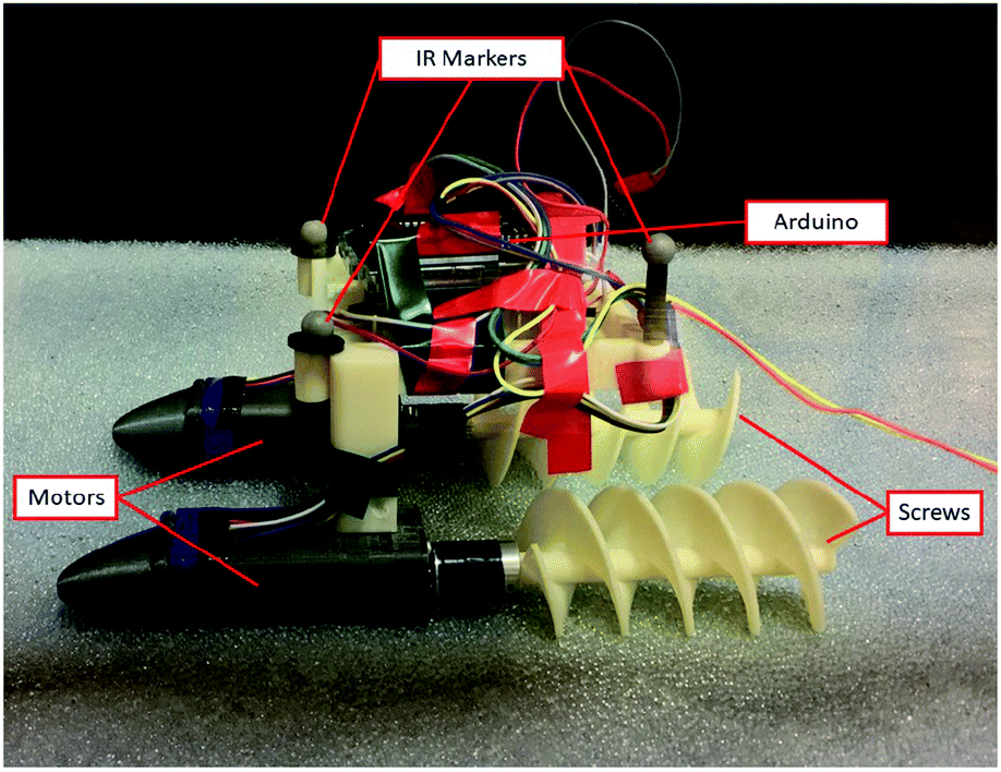 | ||
| Fig. 1 Experimental test craft resting in glass beads with internals exposed. | ||
This craft was then set in a 20 cm by 100 cm bed of 2 mm glass beads using approximately 15 cm of depth. Speed of the motors was directly monitored via encoders during each trial to ensure consistency during testing. Seven speeds were used: 30, 45, 60, 75, 90, 105, and 120 rotations per minute (rpm). P4 spanned 45–120 rpm, P6 spanned 30–120 rpm, and P8 spanned 30–120 rpm. The P4 set of screws had difficulty overcoming initial resistance at 30 rpm and these results were discarded. Each trial ran for approximately 10–15 seconds. The craft was placed on the top of the beads and allowed to rest under its own weight. The glass beads bore the weight of the craft and it did not sink while stationary. It was levelled by observation at the beginning of the run. At the end of the run, the craft would be tilted backwards slightly. This procedure was repeated for the DEM simulations, with the craft initially placed a negligible but non-zero distance above the bed of beads. After ten trials, the Arduino was reprogrammed for the next speed and run again. The motor control and rpm data collection were driven by the Arduino. The craft position was monitored via an Optitrack infrared camera system. Three infrared silver markers were attached to the craft as seen in Fig. 1 and the cameras (not seen here) were mounted to the four corners of the test bed. The Optitrack infrared camera system produced position data of the markers in its calibrated reference frame versus time. Velocity was calculated using distance traveled over time. Initial analysis examined both depth and lateral travel distances and found them negligible. A surface leveling instrument was used after every trial and beads were reset manually to ensure adequate mixing.
2.2 MBD-DEM simulations
The same designs used to manufacture the ABS parts were utilized in the simulations. In DEM, simulation completion time scales exponentially with number of particles. This was something we wished to avoid. Thus, simulation time was reduced by decreasing the dimensions of the simulated bed. The experimental environment was a multi-purpose test bed and therefore arbitrarily large compared to our requirements for avoiding wall effects. During preliminary simulations, we evaluated several simulations which were identical except for incremental narrowing of the bed. We examined the results and chose the smallest size which showed no wall effects. We also used the simulation data to assess the necessary length of the test bed for achieving the steady velocity. The granular environment was set up in a DEM program called EDEM as seen in Fig. 2.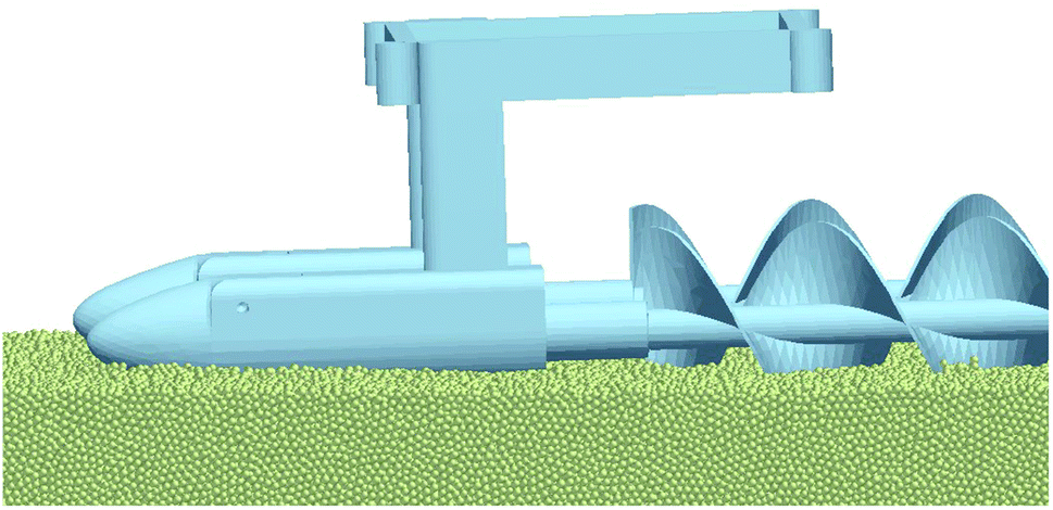 | ||
| Fig. 2 Simulation setup in DEM program showing craft and beads. | ||
DEM simulations allow user control over many aspects of the simulated granular materials and intruder geometry materials. These parameters were set to the best matches found from the literature. Key glass and ABS values are listed in Table 1. Key interaction values are listed in Table 1. A thorough explanation of these values is contained in the results of a static force generation experiment47 but we will discuss these briefly.
| Material property | Glass | ABS |
|---|---|---|
| Poisson's ratio | 0.24 | 0.35 |
| Density (kg m−3) | 2500 | 1070 |
| Young's modulus (Pa) | 7 × 10⁷ | 1.8 × 10⁹ |
| Interactive property | Glass–glass | Glass–ABS |
|---|---|---|
| Coefficient of restitution | 0.97 | 0.7 |
| Coefficient of static friction | 0.16 | 0.174 |
| Coefficient of rolling friction | 2.5 × 10⁻⁵ | 0.162 |
| Other properties | Value |
|---|---|
| Aspect ratio of spheres | 1.1 |
| Average particle size | 2 mm |
| Particle size standard deviation | 0.1 mm |
| Simulation timestep | 4.84 × 10⁻⁶ s |
As discussed before, DEM uses a different approach than analytical methods such as continuum mechanics or empirical approaches. Each individual particle is simulated. The effect of particles on each other is driven by the selection of physics models based on the needs of the user and the attributes of the granular media. Some models incorporate cohesion, adhesion, machine wear, and other aspects. The Hertz–Mindlin physics model was selected based on the need for a robust model without requiring wear, thermodynamics, or additional analysis. The model is built on Hertzian contact theory; since the model is driven by spherical contact, it looks at calculations between two spheres and drives the motion based on Young's modulus, radii, etc. During particle collision, a small overlap representing an estimated real-world deformation is allowed. This allowed deformation is based on the stiffness from the Young's modulus. A smaller allowable deformation requires more frequent checks and hence, a smaller time step and higher frequency. This slows the progress of the simulation and a balance must be struck between implementation and material fidelity. Particles in the simulation were modeled as closely to the glass beads as possible. The aspect ratio of 1.1 means that a small degree of eccentricity was introduced by creating particles in the program which were two slightly offset spheres overlapping each other. The software uses spherical contact physics models and as such, all particles generated are some composition of spherical surfaces. The dynamics of the craft and reaction physics were driven by a multi-body dynamics (MBD) software called Adams.48,49 In the case of MBD-DEM co-simulations, the MBD software will control the movements of the craft. For example, in our case we set the rotational speed of the screws in Adams. The model and physics behind it were then exported to the simulated granular environment. In our case we set the rotational speed of the screws in Adams. Adams simulates the relationship between the solid bodies of the craft dynamic system and their reaction to the environment; it simulates how the craft linkages react to internal linkage forces and external environmental forces. The DEM program, EDEM, simulates how the granular media reacts to the internal granular forces and external geometry forces.50–52 The center of mass in EDEM is co-located at the identical space in the universal coordinate frame as the center of mass in Adams. EDEM calculates how the granular media reacts to the geometric intruder's motion. It then sends reaction forces to the MBD program after a discrete time step. These reaction forces are implemented by Adams onto the craft geometry and translated into movement during each discrete time step. The craft location is adjusted in EDEM, reacts with the granular environment, and this cycle continues until completion of the simulation. Simulations of Earth-gravity experiments were run to compare directly to their experimental counterparts and identify any salient patterns or differences between the two. All simulations were run using the discrete time step listed in Table 1. All simulations ran for a total length of 2.5–3 seconds. This length of time was determined to be the minimal amount of time required to reach steady state velocity.
3 Results and discussion
3.1 MBD-DEM Earth simulations compared to experiments
All results for craft steady state velocity as a function of rpm are shown in Fig. 3. Velocity as a function of rpm had slopes of 0.386, 0.656, and 0.855 for P4, P6, and P8 respectively. This relationship has an observably linear trend. At least four rpm data points for each simulation were also used to establish trends. The craft velocity of each set of simulations was higher than that of the experiments, as observed in the individual pairings. When the slopes of experiment and simulation best fit lines are compared, the increases are 25.3%, 18.5%, and 15.2% for P4, P6, and P8 respectively. In terms of raw inflation between experimental values and simulated for each rpm, the average was 18.3%, 4.5%, and 17.5% respectively. The maximum difference between experiment and simulation data was P4 at 120 rpm. Steady state for experimental was 47.7 mm s−1 while simulation was 59 mm s−1 for a difference of 23.1%. While the simulated values showed inflation, and changed slightly between designs, the overall trends for all simulations and their experimental counterpart were very similar. The R2 values, coefficient of determination, of these fit lines ranges from 0.9967 to 0.9998.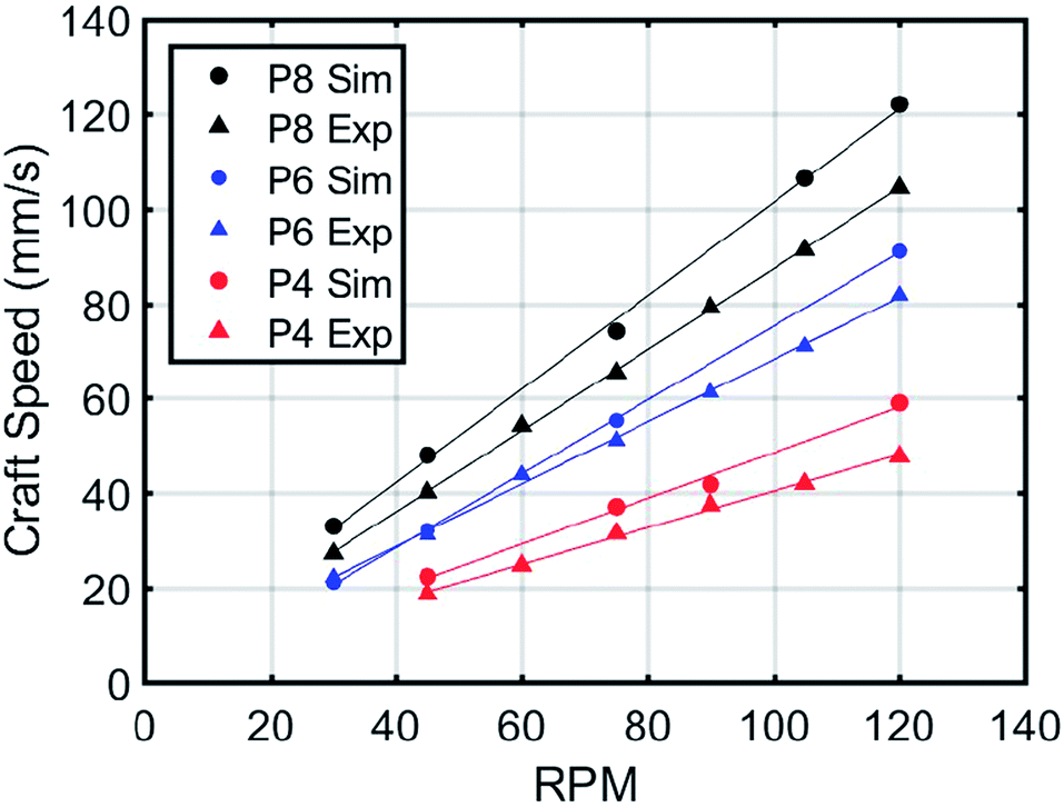 | ||
| Fig. 3 Experiments and simulations compared for three craft designs. | ||
3.2 MBD-DEM Earth simulation slip trends compared to experiments
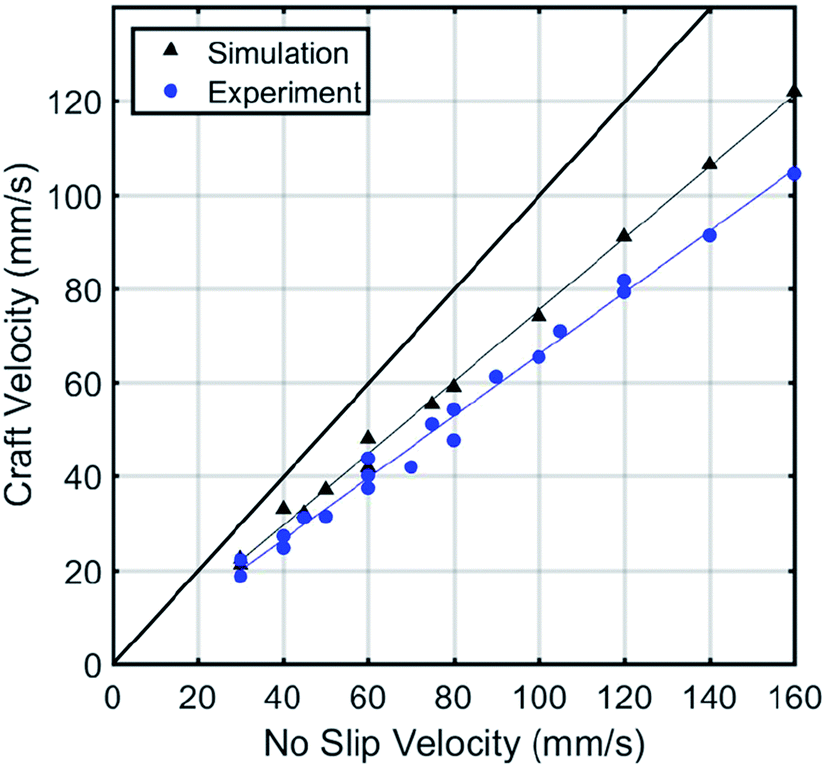
This same data, when converted to no-slip format, also shows uniform trends compared to the experiment as seen in Fig. 4. Imagine a cylinder with helical windings. As this screw rotates in place on its center axis, the real path in space of any arbitrary point on it is a perfect circle around that axis of rotation. Yet when observed rotating, that arbitrary point can appear to move in a forward or backward motion perpendicular to this plane because during rotation, a new portion of the helix has shifted to occupy that control volume. As the pitch of the screw is increased, the rate at which physical blade geometry enters or exits that control volume increases as well. When contact is made with a group of particles, those particles resist the movement of the helical blades within their particular control volume. This reaction force propels the craft forward. We define no-slip velocity as the hypothetical translational velocity achieved if rotational motion is converted to translational without loss.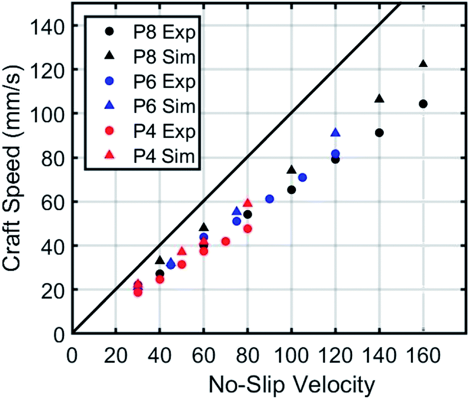 | ||
| Fig. 4 Slip trends shown for individual designs. | ||
For example, if a tire rotates without slipping along the ground, it will translate the distance of one circumference per rotation. For a screw, no slipping would mean a translation of one pitch per rotation. A screw with a 4 cm pitch rotating at 60 rpm (1 rotation per second) would have a no-slip velocity of 4 cm s−1. The pitch couples the rotational and translational movement. Slip, in the context of this paper, is the ratio of the actual craft velocity to the maximum velocity possible if all locomotive efforts were perfectly transferred into translational motion. Let us now take the black triangles of Fig. 4 as an example. The furthest datapoint shows coordinates of approximately (160, 120). This indicates 25% slip because the actual velocity is 75% of the theoretical maximum. If we move several datapoints down the black triangles, we can see a datapoint which looks to be approximately (100, 75). This, again, indicates 25% slip. The ratios of actual velocity to theoretical remain very close and are expressed in that slope. However, the real difference between the theoretical maximum and actual velocity of the two datapoints change. In the slower datapoint, the gap is 25 rpm and in the faster datapoint the gap is 40 rpm.
If the no-slip velocities of all three screws are plotted with their experimental results on one plot as seen in Fig. 4, we can see that the levels of slip experienced between the three designs is quite similar. The overall slope of the experimental data is 0.657 for actual velocity vs. no-slip velocity. All experimentally tested points obey this linear fit, indicating that our experiments were below velocities which would significantly increase slip levels. As the velocity gets higher the linear fit will no longer apply due to the refill rate of the granular media in Earth's gravity. At reduced gravities, this peak velocity and slip begin to change as demonstrated in the reduced gravity section of this article. All tested points demonstrated an observable linear relationship between translational velocity and the no-slip velocity with little variation between the trials for each data point; the largest standard error experienced was 1.9 mm s−1. This data was therefore deemed an acceptable target to validate DEM simulations against.
The thick black line indicates where no-slip velocity would occur. The slope of such velocity would be 1.000 on this graph.
The slope of actual velocity vs. no-slip velocity is 0.761 for all simulation data, an overall increase of 15.8% from the 0.657 for all experimental, as seen in Fig. 5. The simulation data also follows a constant linear trend for slippage. The individual slopes for P4, P6, and P8 in simulation are 0.725, 0.775, and 0.719. This is an increase of 25.6%, 18.1%, and 12.2% for each design respectively over experimental slopes. This means that the simulated craft experienced both (a) closer rates of slip between designs than the experimental cases, and (b) less overall slip during movement than experiments. Several DEM simulation material parameters could be the cause of this variation. The Young's modulus has been purposefully reduced. The rolling or static friction coefficient between glass and ABS are possible causes of differences between simulation and experiments. The surface friction of printed materials may vary with different geometries, printers, and print conditions. There also were no studies found in the literature which explicitly tested printed ABS and glass. The coefficient of restitution was also not found to be explicitly tested. This is another potential cause, but we hypothesize a less likely one since impact speeds in these simulations were low. Furthermore, the modification of Young's modulus is another potential cause. We know that it can modify forces by slightly changing the packing fraction (less rigid material can pack more tightly into the same space) and this gives the screw a more densely packed media to push against. It may also affect drag forces. Finally, the differences could also be explained by the approximations required to use the Hertz–Mindlin physics model in DEM or the choice of time steps.
 | ||
| Fig. 5 Comparison of simulation slip trends with experimental for all designs combined. Actual craft velocity achieved is compared to the hypothetical maximum no-slip velocity. Trend lines of simulations and experiments can be compared to the thick black line, which indicates what a constant, no-slip velocity would look like. | ||
This leads to two insights. First, the data shows that with calibration of simulation parameters to test data, MBD-DEM simulations can reproduce craft movement from shearing, helical geometries in a range of speeds under the assumptions of constant slip. This is while utilizing a Young's modulus reduction technique by several orders of magnitude. The Young's modulus was reduced from a nominal value of 70 GPa to 70 MPa for simulation. Evidence in the literature suggests that bulk behavior may not show significant error until Young's modulus is lowered below the 1 × 10⁷ threshold.53 Second, the choices for glass and ABS material properties, as well as interaction parameters, for these DEM simulations have been successfully validated to a reasonable degree. With Earth gravity validated to within a 15% offset of experimental values, we now move on to a set of computational comparisons which address granular scaling laws with a focus on gravity reduction.
3.3 MBD-DEM lunar and Ceres gravity simulations compared to general scaling relations for varied gravities
Recent granular scaling laws have been developed in the literature which have implications for traversing granular media.46 These have been tested and confirmed for arbitrarily shaped, rotating intruders of uniform thickness in one dimension. This includes a classic wheel shape, a lugged wheel, and even a rotating rectangular bar. The dimensional analysis performed in the literature relies on mass, wheel shape, dimensions, speed, and gravity. First, assume a wheel of arbitrary shape f and let us define the inputs. This wheel has a tire thickness of D into the page. It has a characteristic length L that scales with the shape, typically defined as a radius for circular wheels. The wheel has mass M concentrated on the axle, acted on by constant g gravity. Assume a consistent granular media and a fixed rotational velocity ω. The outputs of interest derived from this are craft mobility power, P, and the wheel's translational velocity V. These outputs are a function of time, t. The non-dimensionalized relationships between these, derived in the cited literature, are as follows:
 | (1) |
If we consider a second wheel of identical shape but different size, it can be scaled in characteristic length by an arbitrary constant r. For example, an increase in the second wheel's radius by 50% results in an r of 1.5. The wheel's mass can be scaled similarly by an arbitrary constant s. After these two constants are chosen, the wheel thickness and velocity can be scaled accordingly:
| (L′, M′, D′, ω′) = (rL, sM, sr−2D, r−1/2ω) | (2) |
Subsequently, this results in a predicted power and velocity scaling:
| P′ = sr1/2P | (3) |
| V′ = r1/2V | (4) |
This set of equations has implications for Earth-based mobility, but the focus of our work's expansion is in further examination of the gravity-variant modification of this law in the literature. By choosing to vary gravity by a constant q, a slightly different set of relationships is presented:
 | (5) |
This results in a different relationship between the variables:
| (g′, L′, M′, D′, ω′) = (qg, rL, sM, sr−2D, q1/2r−1/2ω) | (6) |
This also results in different relationships for output variables as well
| P′ = q3/2r1/2sP | (7) |
| V′ = q1/2r1/2V | (8) |
These were experimentally validated in the literature.46 However, a key feature of the scaling laws is focus on strictly uniform-thickness wheels with the axis of rotation perpendicular to the direction of translational motion. This motion is primarily driven by contact forces with particles near or on the surface of the granular media and to a certain depth based on stress envelopes. In a screw-powered vehicle, the rotating axis is parallel to the direction of translational motion and utilizes an intruder with a different set of reaction forces in the medium. Since screws and augers offer opportunities for mobility, anchoring, and material transfer in both terrestrial and space settings, it is worth examining whether a dynamic scenario can be predicted by these particular laws or not. If shear-dominated motions can be expressed by the same laws, it increases the robustness of these parameters. To simplify examination, we removed the differences of size and mass by setting s = 1 and r = 1 while varying the gravity constant q to 1/6 and 1/36 for lunar and Ceres gravity. This produced a set of test velocities to compare different gravities and predict the power and velocity outcomes in these two reductions of gravity. When gravity and angular velocity are modified but all other quantities are left constant, the relationships reduce to the following:
| (g′, L′, M′, D′, ω′) = (qg, L, M, D, q1/2ω) | (9) |
| P′ = q3/2P | (10) |
| V′ = q1/2V | (11) |
Bearing these scaling laws in mind, speeds were identified for both gravity levels. The simulations were run for three gravity levels. The original simulations at Earth gravity served as the first. The second was lunar gravity (1.62 m s−2). The third was Ceres gravity (0.27 m s−2), the largest object in our asteroid belt. This was done because the Earth–Moon gravity ratio is very similar to the Moon–Ceres ratio (1/6). All EDEM parameters regarding material parameters were kept constant. As can be seen in Fig. 7, the craft obeyed the predictions set out by the scaling laws for lunar gravity in both velocity and power. Velocity in this case is defined as the translational velocity in the primary direction of travel. Power in this case is mechanical power, the rate of physical work being done by the screws. These are both results which EDEM allows the user to extract on a per-geometry basis. These showed very close approximations of 102.6%, 105.9% and 102.7% of predicted values for 12, 30, and 45 rpm respectively. The power was also close, with 94.2% 92.1% and 94.4% of predicted values. The perfect prediction lines have been shown in black on these graphs.
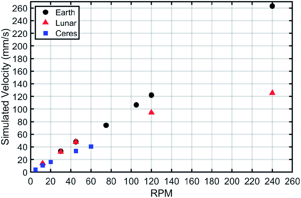 | ||
| Fig. 6 Simulations of identical geometry with three gravity variations. | ||
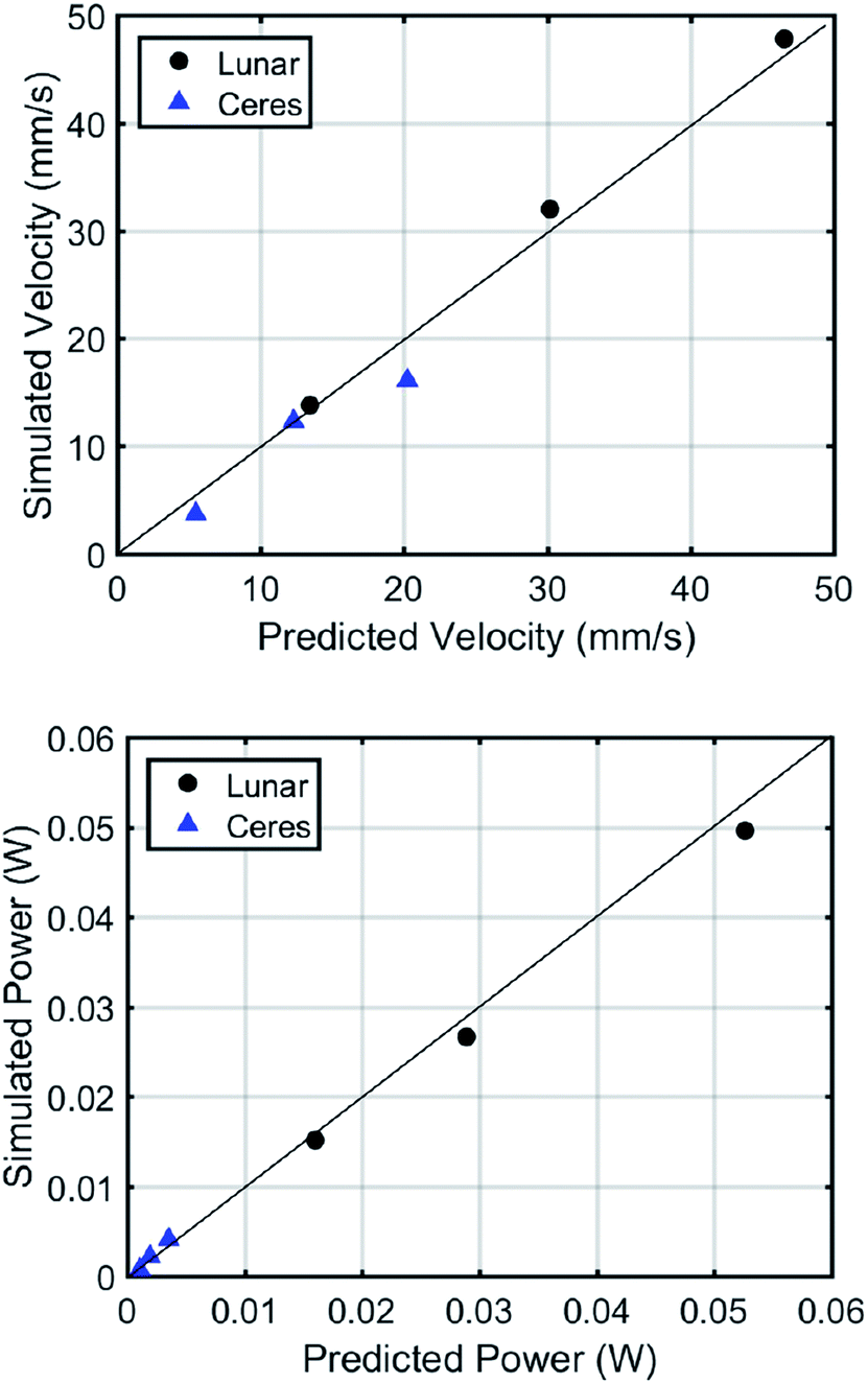 | ||
| Fig. 7 Scaling law predictions versus simulation results. | ||
The Ceres gravity resulted in significant variation for predicted values compared to simulated. The 12 rpm case showed a 0.1% deviation from the expected velocity, but the 5 rpm case was 67.5% of predicted value and the 20 rpm case was 79.5% of the predicted value. In the case of power, 62.5%, 109.4%, and 114.9% were the values found as a percent of predicted value. One item to note is that the gravity variation performed in the scaling literature was done so with a gravity increase, not decrease. As such, we believe we encountered a level of gravity low enough that our speeds do not stay in a constant-slip range.
In Fig. 6, the raw craft velocities versus their rotation speeds are plotted for all gravity levels. While the Earth and lunar gravity simulations show almost identical relationships, the Ceres gravity simulation speeds display a non-linear trend. The trends clearly show further deviation with increased speeds. The lower gravity provides less entrapped granular media to push against.
4 Potential sources of error
The errors in this paper fall into two categories. The first set of differences occurs between experimental and simulated craft at Earth gravity. The second occurs between simulated and predicted values at reduced gravity compared to Earth gravity.To address the small but non-trivial differences in experimental validation, it is worth noting the driving physics behind the DEM simulations. Each individual particle was modeled and driven by the listed granular parameters, as well as a Hertz–Mindlin physics model for spherical contact. A typical technique for DEM is to reduce the Young's modulus for faster simulation time.53 While the change in Young's modulus from its real-world measured value to a reduced one does show some level of effect on the simulations, the effect appears consistent. This reduced modulus was used for all simulations.
Since the Earth-DEM simulations showed close patterns to experiments, we consider them valid for evaluating scaling law comparisons. They have relatively consistent inflation between their velocity measurements and behaved as expected. The lunar gravity DEM simulations also behaved as expected. However, the Ceres simulations (performed under 3% of Earth's gravity) did not follow predictions. The most likely cause, as is observable from the trends, is that an assumption of constant slip rate is necessary for these laws to work. As gravity is decreased and granular media is subject to weak compaction, the range of speeds in which slip stays constant shrinks considerably and in this case, tested speeds exceeded it.
5 Conclusion
This study presents experimental and DEM simulation comparisons of a double-helix Archimedes screw propelled vehicle traveling in a bed of soda-lime glass beads. Three screws of different pitch lengths were tested at six speeds in ten trials for a total of 180 experiments using an Optitrack infrared system to measure craft velocity. These experiments were then replicated in co-simulations using EDEM and Adams software. DEM simulation results for thrust forces in the 30–120 rpm regime had a 15–20% increase of velocity in direction of travel compared to experiment. The experimental results suggest that stiffness-reduced DEM simulations provide reliable dynamic velocity prediction. We also examined recently developed wheeled granular scaling laws and applied gravity variation to three-dimensional screws in Earth, Moon, and Ceres simulated gravity. The preliminary results indicate that they obey the developed scaling laws under conditions of consistent slip.This opens several future paths. One is the characterization of lunar simulants for DEM simulations. While these particles typically exist in size on the order of 100 microns, there have been studies which show that scaling small cohesive particles up to an acceptable size for simulation still results in accurate predictions of forces on agricultural tools at a macroscopic level.54 Another path is the exploration of surface level dynamic tests with an SPV on cohesive granular media. This could provide valuable insight to the mobility of vehicles as well as the excavation of this material. The last path is further development of the current granular scaling laws as they apply to other geometries, granular media, and testing of gravity and higher velocity effects. We also seek to evaluate the effects of various levels of Young's modulus reduction.
Conflicts of interest
There are no conflicts to declare.Acknowledgements
The authors would like to thank Arizona State University for funding, the BIRTH Lab members for fruitful discussion, and Professor Heather Emady for insights.References
- H. Marvi, C. Gong, N. Gravish, H. Astley, M. Travers, R. L. Hatton, J. R. Mendelson, H. Choset, D. L. Hu and D. I. Goldman, Science, 2014, 346, 224–229 CrossRef CAS PubMed.
- M. Grujicic, H. Marvi, G. Arakere, W. Bell and I. Haque, Multidiscip. Model. Mater. Struct., 2010, 6, 229–256 CrossRef.
- M. Grujicic, H. Marvi, G. Arakere and I. Haque, Multidiscip. Model. Mater. Struct., 2010, 6, 284–308 CrossRef.
- A. Thoesen, S. Ramirez and H. Marvi, 2018 IEEE International Conference on Robotics and Automation, ICRA, 2018, pp. 1–6 Search PubMed.
- H. Bagheri, V. Taduru, S. Panchal, S. White and H. Marvi, Conference on Biomimetic and Biohybrid Systems, 2017, pp. 13–24 Search PubMed.
- S. Kamath, A. Kunte, P. Doshi and A. V. Orpe, Phys. Rev. E: Stat., Nonlinear, Soft Matter Phys., 2014, 90, 062206 CrossRef PubMed.
- K. Kamrin, Int. J. Plast., 2010, 26, 167–188 CrossRef CAS.
- S. Lee and D. B. Marghitu, Int. J. Mech. Sci., 2009, 51, 881–887 CrossRef.
- H. Omori, T. Murakami, H. Nagai, T. Nakamura and T. Kubota, Aerospace Conference, 2013 IEEE, 2013, pp. 1–9 Search PubMed.
- P. Tahmasebi, M. Sahimi and J. E. Andrade, Geophys. Res. Lett., 2017, 44, 4738–4746 CrossRef.
- M. Neumeyer and B. Jones, J. Terramechanics., 1965, 2, 83–88 CrossRef.
- K. Evans, J. Sustain. Met., 2016, 2, 316–331 CrossRef.
- A. Koshurina, M. Krasheninnikov and R. Dorofeev, Procedia Eng., 2016, 150, 1263–1269 CrossRef.
- M. Michael, F. Vogel and B. Peters, Comput. Methods Appl. Mech. Eng., 2015, 289, 227–248 CrossRef.
- J. B. Johnson, P. X. Duvoy, A. V. Kulchitsky, C. Creager and J. Moore, J. Terramechanics., 2017, 73, 61–71 CrossRef.
- T. Leblicq, S. Vanmaercke, H. Ramon and W. Saeys, Int. J. Mech. Sci., 2015, 94, 75–83 CrossRef.
- P. M. Pieczywek and A. Zdunek, Soft Matter, 2017, 13, 7318–7331 RSC.
- Y. Guo, C. Wassgren, W. Ketterhagen, B. Hancock and J. Curtis, Soft Matter, 2018, 14, 2923–2937 RSC.
- E. J. Parteli and T. Pöschel, Powder Technol., 2016, 288, 96–102 CrossRef CAS.
- H. Xin, W. Sun and J. Fish, Int. J. Mech. Sci., 2018, 149, 373–392 CrossRef.
- R. Yoshimatsu, N. A. Araújo, T. Shinbrot and H. J. Herrmann, Soft Matter, 2016, 12, 6261–6267 RSC.
- X. Li, W. Li, S. Yang, Z. Hao and H. Shi, Int. J. Mech. Sci., 2018, 138, 250–261 CrossRef.
- W. Liu, S. Li, A. Baule and H. A. Makse, Soft Matter, 2015, 11, 6492–6498 RSC.
- M. Z. Miskin and H. M. Jaeger, Soft Matter, 2014, 10, 3708–3715 RSC.
- H. Zhao, X. An, D. Gou, B. Zhao and R. Yang, Soft Matter, 2018, 14, 4404–4410 RSC.
- F. Verbücheln, E. J. Parteli and T. Pöschel, Soft Matter, 2015, 11, 4295–4305 RSC.
- D. K. A. Patel, B. P. Patel and M. K. A. Pate, International Journal of Mechanical Engineering and Robotics Research, 2015, 4, 188 Search PubMed.
- M. K. Al-Solihat and M. Nahon, Int. J. Mech. Sci., 2018, 142, 518–529 CrossRef.
- O. Kudryavtsev and S. Sapozhnikov, Int. J. Mech. Sci., 2016, 114, 60–70 CrossRef.
- B. Harthong, J.-F. Jérier, V. Richefeu, B. Chareyre, P. Dorémus, D. Imbault and F.-V. Donzé, Int. J. Mech. Sci., 2012, 61, 32–43 CrossRef.
- J. Wong, J. Terramechanics., 2012, 49, 49–61 CrossRef.
- T. Kobayashi, Y. Fujiwara, J. Yamakawa, N. Yasufuku and K. Omine, J. Terramechanics., 2010, 47, 261–274 CrossRef.
- M. Jebahi, J.-L. Charles, F. Dau, L. Illoul and I. Iordanoff, Comput. Methods Appl. Mech. Eng., 2013, 255, 196–209 CrossRef.
- S. Ferson, W. L. Oberkampf and L. Ginzburg, Comput. Methods Appl. Mech. Eng., 2008, 197, 2408–2430 CrossRef.
- A. Mesgarnejad, B. Bourdin and M. Khonsari, Comput. Methods Appl. Mech. Eng., 2015, 290, 420–437 CrossRef.
- L. A. Petri, P. Sartori, J. K. Rogenski and L. F. de Souza, Comput. Methods Appl. Mech. Eng., 2015, 291, 266–279 CrossRef.
- I. Arias, J. Knap, V. B. Chalivendra, S. Hong, M. Ortiz and A. J. Rosakis, Comput. Methods Appl. Mech. Eng., 2007, 196, 3833–3840 CrossRef.
- M. A. Cruchaga, C. M. Muñoz and D. J. Celentano, Comput. Methods Appl. Mech. Eng., 2008, 197, 2823–2835 CrossRef.
- R. D. Maladen, Y. Ding, P. B. Umbanhowar, A. Kamor and D. I. Goldman, J. R. Soc., Interface, 2011, 8, 1332–1345 CrossRef PubMed.
- Y. Ding, S. S. Sharpe, A. Masse and D. I. Goldman, PLoS Comput. Biol., 2012, 8, e1002810 CrossRef CAS PubMed.
- C. Li, T. Zhang and D. I. Goldman, science, 2013, 339, 1408–1412 CrossRef CAS PubMed.
- T. Zhang and D. I. Goldman, Phys. Fluids, 2014, 26, 101308 CrossRef.
- Y. O. Aydin, B. Chong, C. Gong, J. M. Rieser, J. W. Rankin, K. Michel, A. G. Nicieza, J. Hutchinson, H. Choset and D. I. Goldman, Conference on Biomimetic and Biohybrid Systems, 2017, pp. 595–603 Search PubMed.
- S. Dunatunga and K. Kamrin, J. Fluid Mech., 2015, 779, 483–513 CrossRef CAS.
- S. Dunatunga and K. Kamrin, J. Mech. Phys. Solids, 2017, 100, 45–60 CrossRef CAS.
- J. Slonaker, D. C. Motley, Q. Zhang, S. Townsend, C. Senatore, K. Iagnemma and K. Kamrin, Phys. Rev. E, 2017, 95, 052901 CrossRef PubMed.
- A. Thoesen, S. Ramirez and H. Marvi, AIChE J., 2019, 65, 894–903 CrossRef CAS.
- X. Wang, S. Yang, W. Li and Y. Wang, Int. J. Adv. Manuf. Technol, 2018, 96, 1175–1185 CrossRef.
- Y. Ko and C. Song, Int. J. Auto. Tech., 2010, 11, 339–344 CrossRef.
- X. J. Wang, Y. L. Chi, W. Li, T. Y. Zhou and X. L. Geng, Advanced Materials Research, 2012, pp. 1395–1398 Search PubMed.
- R. Briend, P. Radziszewski and D. Pasini, Can. Aeronaut. Space J., 2011, 57, 59–64 CrossRef.
- Y. Chung and J. Ooi, Modern Trends in Geomechanics, Springer, 2006, pp. 223–239 Search PubMed.
- S. Lommen, D. Schott and G. Lodewijks, Particuology, 2014, 12, 107–112 CrossRef.
- M. Ucgul, J. M. Fielke and C. Saunders, Information Processing in Agriculture, 2015, 2, 130–141 CrossRef.
Footnote |
| † Electronic supplementary information (ESI) available. See DOI: 10.1039/c9ra00399a |
| This journal is © The Royal Society of Chemistry 2019 |