
 Open Access Article
 This Open Access Article is licensed under a Creative Commons Attribution-Non Commercial 3.0 Unported Licence
Machine learning algorithms enhance the specificity of cancer biomarker detection using SERS-based immunoassays in microfluidic chips†
Nariman Banaei a,
Javad Moshfeghb,
Arman Mohseni-Kabirc,
Jean Marie Houghtond,
Yubing Sun*aef and
Byung Kim*af
a,
Javad Moshfeghb,
Arman Mohseni-Kabirc,
Jean Marie Houghtond,
Yubing Sun*aef and
Byung Kim*af
aDepartment of Mechanical and Industrial Engineering, University of Massachusetts, Amherst, Amherst, MA, USA. E-mail: ybsun@umass.edu; kim@engin.umass.edu
bDepartment of Electrical and Computer Engineering, University of Massachusetts, Amherst, MA, USA
cDepartment of Physics, University of Massachusetts, Amherst, MA, USA
dDepartment of Medicine, University of Massachusetts Medical School, Worcester, MA, USA
eDepartment of Chemical Engineering, University of Massachusetts, Amherst, Amherst, MA, USA
fInstitute for Applied Life Sciences, University of Massachusetts, Amherst, Amherst, MA, USA
First published on 15th January 2019
Abstract
Specificity is a challenge in liquid biopsy and early diagnosis of various diseases. There are only a few biomarkers that have been approved for use in cancer diagnostics; however, these biomarkers suffer from a lack of high specificity. Moreover, determining the exact type of disorder for patients with positive liquid biopsy tests is difficult, especially when the aberrant expression of one single biomarker can be found in various other disorders. In this study, a SERS-based protein biomarker detection platform in a microfluidic chip and two machine learning algorithms (K-nearest neighbor and classification tree) are used to improve the reproducibility and specificity of the SERS-based liquid biopsy assay. Applying machine learning algorithms to the analysis of the expression level data of 5 protein biomarkers (CA19-9, HE4, MUC4, MMP7, and mesothelin) in pancreatic cancer patients, ovarian cancer patients, pancreatitis patients, and healthy individuals improves the chance of recognition for one specific disorder among the aforementioned diseases with overlapping protein biomarker changes. Our results demonstrate a convenient but highly specific approach for cancer diagnostics using serum samples.
1. Introduction
Early diagnosis would significantly decrease the mortality from cancer prior to the onset of metastasis with removal surgery or even at the early initiation of metastasis with current common therapies such as chemotherapy and cytotoxic drugs.1–4 Liquid biopsy is an emerging non-invasive diagnosis approach which can be used as an inexpensive early detection tool and an alternative to cumbersome imaging and tissue biopsy techniques.5,6 The high cost and invasive nature of conventional tissue biopsies prevent them from being standard screening tests for normal adults. Recent studies demonstrated that liquid biopsies have potential to diagnose adenovirus infection,7 lung cancer,8 breast cancer,9 lung cancer,8 breast cancer9 and ovarian cancer (OVC).10One of the major challenges that bottleneck the broad applications of the liquid biopsy in cancer screening is the lack of specificity. So far, only a few protein biomarkers have been approved by the FDA for use in cancer diagnostics. However, these biomarkers are often non-specific to a certain type of cancer. For example, CA19-9 is the only validated serum biomarker for pancreatic cancer (PC). However, CA19-9 also elevates in patients with OVC11 and chronic pancreatitis.12 Similarly, human epididymis protein 4 (HE4), an approved serum biomarker for OVC,13,14 is also overexpressed in patients with PC,15,16 endometrial cancer,17 and lung cancer.18,19 MMP-7,![[thin space (1/6-em)]](https://www.rsc.org/images/entities/char_2009.gif) 20–22 MUC-423,24 and mesothelin25,26 are some other examples of potential biomarkers for PC have also been identified as potential biomarkers for OVC.27–29 Thus, relying on a single biomarker for cancer diagnostics has limited success.
20–22 MUC-423,24 and mesothelin25,26 are some other examples of potential biomarkers for PC have also been identified as potential biomarkers for OVC.27–29 Thus, relying on a single biomarker for cancer diagnostics has limited success.
Current strategies to improve the specificity of liquid biopsy is to detect various types of biomarkers not limited to proteins, but also including microRNAs, circulating tumor DNA, etc.30,31 Although this approach significantly improves the detection specificity, multiple detection methods such as immunoassays and PCR are required, limiting its application in resource-limited settings.
We recently reported a Surface Enhanced Raman Spectroscopy (SERS)-based immunoassay for detecting several biomarkers of PC in sera.32 SERS can provide intrinsic fingerprint information of samples with high sensitivity.33 The SERS technique has evolved as one of the most suitable candidates for the multiplex detection,34,35 due to the sharp and narrow spectra and multiple signatures of Raman spectra.36 SERS has been widely used for the detection of cancer biomarkers.37,38 Although SERS is a promising way for biomarker detection, a quantitative assessment of SERS is difficult, partially due to the poor reproducibility.39,40 This is because SERS-based immunoassays using conventional immobilization of functionalized gold particles (NPs) are often associated with technical issues such as the inhomogeneous distribution of NPs on substrates during multiple manual washing steps.40 It has been suggested that a highly sensitive and reproducible SERS-based analysis can be addressed if a continuous flow and homogeneous mixing conditions are maintained.39
In this work, we reported a SERS-base multiplex protein biomarker detection platform in a microfluidic chip to detect several protein biomarkers of OVC, PC, and pancreatitis (CA19-9, HE4, MUC4, MMP7, and mesothelin). The microfluidic platform significantly improved the reproducibility of the assay, and multiplex detection can improve the specificity for cancer detection. We further employed machine learning algorithms to predict the type of disease and find critical biomarkers among multiple biomarkers to distinguish between diseases with similar biomarkers (PC, OVC, and pancreatitis). Decision tree and K nearest neighbor classification methods are used in this analysis. Together, we demonstrated a convenient but highly specific approach for cancer diagnostics using serum samples.
2. Experimental details
2.1 Reagent
Gold nanoshells (660 nm resonant, 151 nm diameter, 3.7 × 10¹⁰ particles per mL and 800 nm resonant), was purchased from NanoComposix. Sodium chloride, StartingBlock, and borate buffer (50 mM) were obtained from ThermoFisher Scientific. Dithiobis-(succinimidyl propionate) (DSP), dimethylsulfoxide (DMSO), 4-nitrobenzenethiol (4-NBT), acetonitrile, phosphate buffered saline (PBS), and bovine serum albumin (BSA) were acquired from Sigma Aldrich.In our microfluidic SERS-based immunoassay, five different sets of monoclonal antibodies were used to modify the capture substrate and extrinsic Raman labels (ERLs). HE4 antibody was purchased from Proteintech, anti-mesothelin antibody and monoclonal anti-MUC4 were obtained from Abcam, lyophilized MMP7 mAb was purchased from R&D Systems. The CA19-9 antibody was purchased from LifeSpan Bioscience.
2.2 Preparation of ERL
The preparation of antibody-conjugated ERLs has been described previously32 and also is illustrated in Fig. 1. Specifically, modified gold nanoshell as ERL is exploited to provide more intense Raman signal and immunopositivity. In this paper, gold particles were modified with two different thiols, DSP and 4-NBT. DSP has both disulfide and succinimidyl functionalities for chemisorption onto the gold and facile covalent binding of antibodies to the gold particles and substrate; however, DSP does not show intrinsically intense Raman signal. 4-NBT, on the other hand, has been used to provide intense Raman signal due to aryl nitro group with an intrinsically strong Raman active vibrational mode. 4-NBT also contains a disulfide group for spontaneous chemisorption to the gold particles.41 Preparation of ERLs is described as follows: 1.0 mL suspension of gold nanoshells, 40 μL of 50 mM borate buffer, 2.0 μL of 1.0 mM DSP in DMSO and 8.0 μL of 1.0 mM 4-NBT solution in acetonitrile were mixed and left to react for 8 h. To discard excess thiols, the suspension was centrifuged at 2000g for 10 min, and the supernatant was removed with a syringe. Gold nanoshells were resuspended in 2.0 mM borate buffer. ERL preparation was continued by adding 20 μg of MMP7, MUC4, HE4, Mesothelin or CA19-9 primary antibodies to the suspension and incubating for 16 h at 4 °C. Next, 100 μL of 10% BSA was added to the suspension for stabilizing the suspension and blocking nonspecific binding sites and unreacted succinimidyl for 8 hours. After interaction between ERL and blocking buffer, the solution needs to be rinsed three times. For the rinsing process, the suspension was centrifuged, and after decanting the clear supernatant, the loose red sediment was resuspended in 1.0 mL of 2.0 mM borate buffer containing 1% BSA. The triple-rinsed ERL pellet was then resuspended in 0.5 mL of 2.0 mM borate buffer containing 1% BSA to have a final solution with the desired concentration of gold nanoparticles. Finally, the suspension was modified with 50 μL of 10% NaCl for stabilization and then passed through a 0.22 μm syringe filter to remove any large aggregate.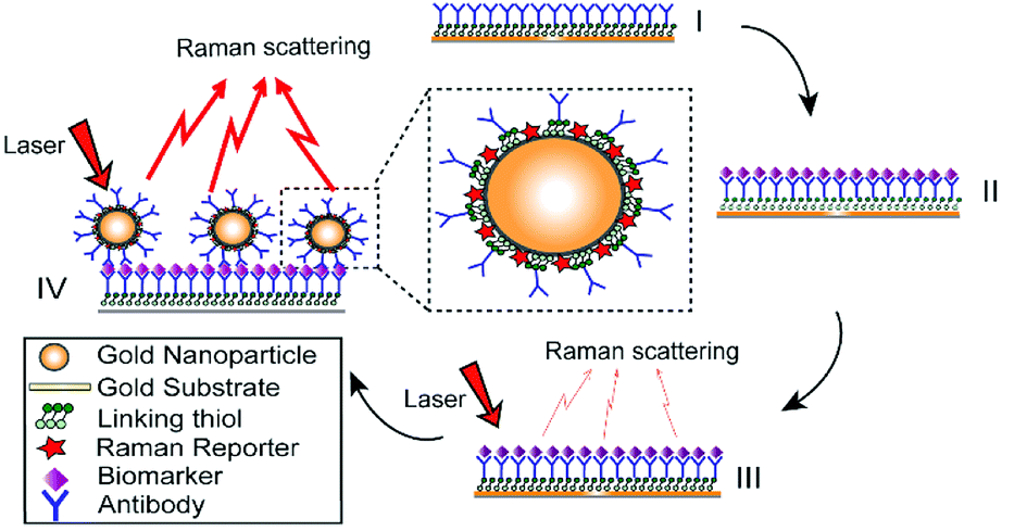 | ||
| Fig. 1 A SERS-based immunoassay for biomarker quantification: (I) functionalizing gold substrate with thiol and antibody; (II) capturing desired antigens from the serum; (III) Raman signal is weak without ERL (IV) loading antibody-conjugated ERL to enhance Raman signal, gold nanoparticles were modified with antibody and Raman reporter. | ||
2.3 Functionalizing capture substrate and microfluidic immunoassay procedures
The optimization of ERL's Raman signal has been described previously.32 We systematically examined the effects of gold particle size, the gap distance between the immobilized particle and the underlying substrate, and substrate materials on the amplification of Raman signals and demonstrated that immobilization of functionalized gold nanoshells with a resonance wavelength of 660 nm on the gold-coated silicon substrate leads to a significant improvement of SERS signals. Thus, we will use gold nanoshells with a resonant wavelength of 660 nm coupled with the gold-coated silicon substrate in our following studies.As shown in Fig. 2, the substrate was immersed in 1 mM DSP in ethanol for 10 h and then rinsed with ethanol and dried under a stream of air. As a result, a layer of DSP is formed on the gold substrate. The microfluidic method is used to provide on-chip flow with sequential injections. Polydimethylsiloxane (PDMS) replica molding from a 3D printed mold was used to fabricate a microfluidic device. PDMS stamps were fabricated by pouring a 10:1 (w/w) mixture of Sylgard 184 elastomer and curing agent and mixture were cured for 1 h at 80 °C. Patterned PDMS was then attached to the DSP coated gold substrate. Capture addresses were filled with 20 μL, 100 μg mL−1 antibody as the first injection. DSP coated substrate was then reacted with the antibody for 6 h. Thus, a capture antibodies layer was formed by attaching to succinimidyl ester of DSP on the substrate. Antibody was then rinsed by injection of 10 mM PBS. Next, 10 μL of StartingBlock blocking buffer was injected to each address to react for 10 h; then the capture substrates were ready to use.
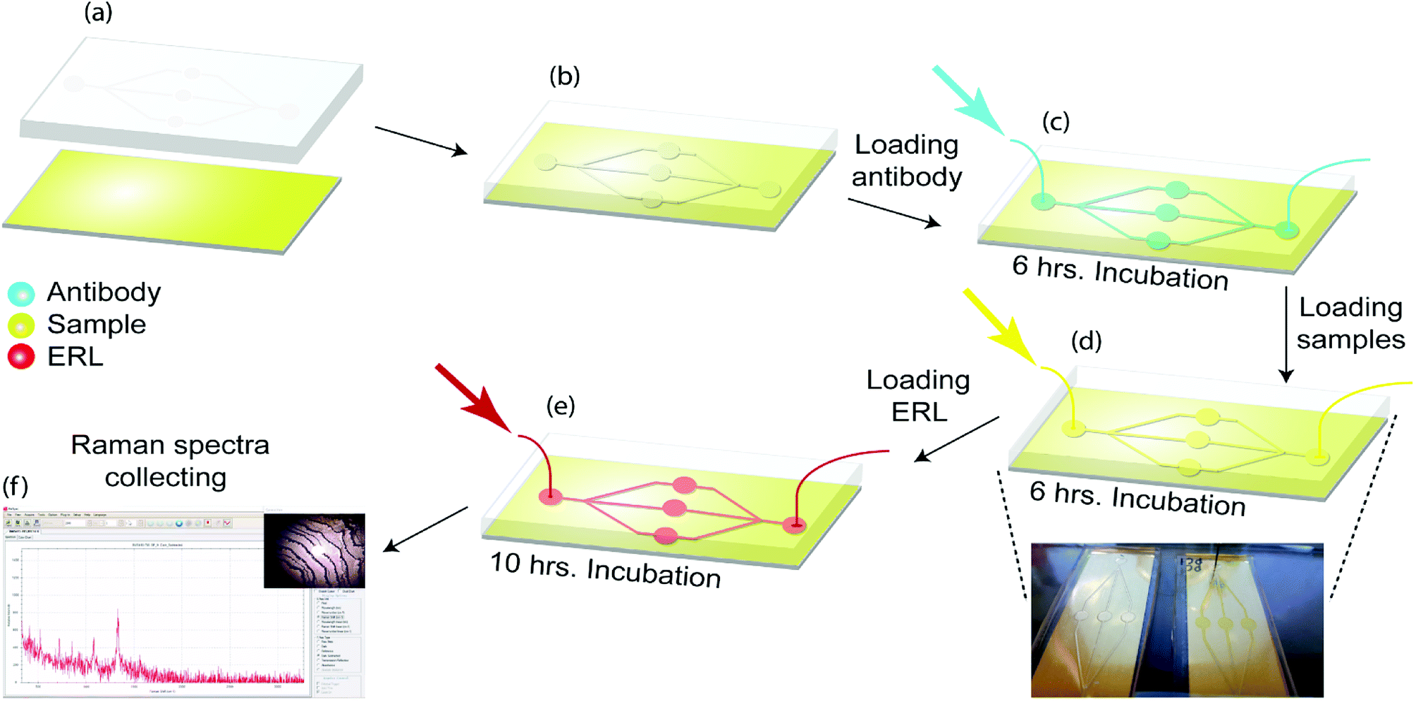 | ||
| Fig. 2 A microfluidic SERS-based immunoassay approach for the multiplex detection of CA19-9, HE4, mesothelin, MMP7 and MUC4 levels in serum samples (a) PDMS replica molding from a 3D printed mold was used to fabricate a microfluidic device. PDMS replicated with one closed and open surface. (b) Patterned PDMS is attached to gold coated microscope slide. (c) 10 μL, 100 μg mL−1 antibodies were loaded in to the capture addresses, the addresses were then exposed with blocking buffer (d) serum samples and (e) ERL. (f) Finally, Raman signals from 10 random positions were collected from each capture address. | ||
After ERL and capture substrates functionalization, the substrates should be loaded with samples. 10 μL of undiluted clinical samples sera were injected in the device and after 6 h incubation was rinsed with buffer (2 mM borate, 150 mM NaCl).
Captured antigens were then labelled by injecting addresses with 10 μL of related ERL suspension for 10 h (Fig. 2). Finally, the substrates were rinsed with buffer (2 mM borate, 150 mM NaCl) and analyzed by the Raman device.
2.4 SERS readout instrumentation
All the measurements and Raman spectra collection were performed with portable BWS415 i-Raman from B&W TEK Co. The incident laser light was focused to 85 μm spot size on the substrate normal incidence. The working distance is 5.9 mm. The light source has a power of 499.95 mW, and an excitation wavelength of 785 nm and the same objective was used to collect the scattered radiation. The antigen concentration was quantified using (vs(NO2)) of 4-NBT intensity at the 1336 cm−1. For reproducibility, three addresses were measured for each concentration and total of 10 readouts on each sample's biomarker.2.5 Patient sample collection and samples characteristics
Under an IRB approved protocol, patients with pancreatic cancer, benign pancreatic disease, and normal control patients were identified from the UMass Memorial Medical Center Chemotherapy Infusion Center and Gastroenterology Clinics. Patients were identified from a review of the weekly schedules, and consecutive patients were enrolled to avoid bias. Patient gender, age, and clinical samples characteristics are shown in Table 1. Sera samples (4 mL serum per patient) were collected and immediately processed/frozen for analysis. Five ovarian cancer samples were purchased from Innovative Research.| Serum sample | Sex/age | Sample characteristics |
|---|---|---|
| PC #1 | F/38 | Metastatic pancreatic adenocarcinoma |
| PC #2 | F/58 | Metastatic pancreatic adenocarcinoma |
| PC #3 | M/61 | Metastatic pancreatic adenocarcinoma |
| PC #4 | F/88 | Locally advanced pancreatic cancer |
| PC #5 | M/57 | Metastatic pancreatic adenocarcinoma |
| Pancreatitis #1 | M/41 | Acute pancreatitis-gallstone disease |
| Pancreatitis #2 | F/55 | Chronic pancreatitis-autoimmune |
| Pancreatitis #3 | M/61 | Chronic pancreatitis-alcohol related |
| Pancreatitis #4 | F/43 | Chronic pancreatitis-hereditary, cystic fibrosis gene mutation |
| Pancreatitis #5 | M/55 | Chronic pancreatitis-alcohol related |
| OVC #1 | F/57 | Endometrioid adenocarcinoma of the ovary |
| OVC #2 | F/59 | Adenocarcinoma, invasive of the ovary |
| OVC #3 | F/62 | Serous carcinoma of the ovary |
| OVC #4 | F/50 | Adenocarcinoma, mucinous type of the ovary |
| OVC #5 | F/59 | Endometrioid carcinoma of the ovary |
| Control | M:F 3:2/age 53–75, average 62 |
3. Results and discussion
3.1 Microfluidic and SERS signal
To investigate the effect of microfluidic approach on the reproducibility of the Raman signal, CA19-9 in serum samples of PC/pancreatitis patients and healthy individuals were detected, and the Raman intensities obtained from the on-chip assay is compared with conventional assay using either a handheld Raman probe or a Raman microscope (Fig. 3a). Notably, the measurement variation of the microfluidic assay reduced to about 50% of the variation of the conventional assays (Fig. 3b). For reproducibility, each microfluidic unit contained three addresses to capture one single biomarker from one serum sample. Thus, for each serum sample (including control, PC, ovarian cancer, and pancreatitis), five microfluidic units were used to detect five different biomarkers (CA19-9, HE4, mesothelin, MMP7, and MUC4). Total of 10 Raman signals were collected from each microfluidic unit.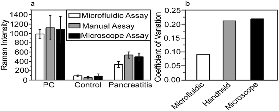 | ||
| Fig. 3 (a) Raman intensity obtained using different approaches. (b) Coefficient of variation (CV) of different approaches, which is calculated by the ratio of the standard deviation to the mean. | ||
3.2 Detection of ovarian and pancreatic cancer biomarkers in patients samples
In our previous work, we have established the standard curve by measuring the Raman intensities using pooled human sera spiked with different concentration of proteins.32 We further used microfluidic SERS-based immunoassay to detect five potential biomarkers (CA19-9, HE4, mesothelin, MMP7, MUC4) from a total of 20 sera samples including five from normal individuals, five from patients with various types of pancreatitis but not PC, five from PC patients and five from ovarian cancer patients. Raman spectra of five selected biomarkers in clinical sera samples are shown in Fig. 4 and ESI Fig. 1.†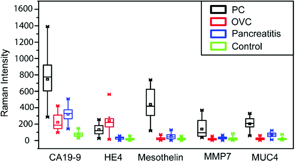 | ||
| Fig. 4 Multiplex detection of CA19-9, HE4, mesothelin, MMP7 and MUC4 levels in serum of normal, PC, ovarian cancer and pancreatitis samples (total of 20 sera samples) using the microfluidic SERS-based immunoassay. Raman intensities of 4-NBT (1336 cm−1) corresponded to CA19-9, HE4, mesothelin, MMP7 and MUC4 in serum samples. Each box represents 50 readouts. | ||
It appears that CA19-9 is the most sensitive biomarker with the highest expression level in almost all patient samples, and other biomarkers, by themselves, cannot distinguish the PC and OVC. Thus, to fully leverage the data obtained from multiple biomarkers for a more accurate prediction, more comprehensive data analysis is needed.
3.3 Data analysis
We next sought to use machine earning based approach to analyze the Raman intensity data we obtained to provide a better prediction of the condition of patients. We first processed the raw Raman spectrum data to reduce the noise level. As the background noise level in SERS signals is relatively low compared with the strongly enhanced peak signals, we applied a simple Fast Fourier Transform (FFT) to the Raman intensity data three times to reduce the noise and smooth the Raman spectrum. The original and denoised spectra of CA19-9 for a pancreatic cancer sample are plotted in Fig. 5(a) and (b) respectively. Fig. 5(c) also demonstrates the original and denoised spectrum together for a better comparison. The processed Raman spectrum of each measurement of biomarker b on patient i is denoted by Rbi,s(![[small nu, Greek, tilde]](https://www.rsc.org/images/entities/i_char_e0e1.gif) ), as a function of wavelength discretized with 1783 points. Measured biomarkers include CA19-9, HE4, mesothelin, MMP7, and MUC4. Performing ten measurements for each of the 20 individual samples and five biomarkers, the dataset includes 1000 Raman spectra Rbi,s().
), as a function of wavelength discretized with 1783 points. Measured biomarkers include CA19-9, HE4, mesothelin, MMP7, and MUC4. Performing ten measurements for each of the 20 individual samples and five biomarkers, the dataset includes 1000 Raman spectra Rbi,s().
 | ||
| Fig. 5 Pre-processing of Raman spectrum. (a) The measured Raman spectrum; (b) the denoised spectrum using FFT filter; (c) the original and denoised spectrum together. | ||
Two supervised algorithms are employed to classify the condition of the patients. First, the Raman spectra peak values Rbi,s() are used for decision tree classifiers, which are fast, simple, and provide useful information about the importance of biomarkers. However, since a single peak value at r = 1500 cm−1, the resonance wavelength of Raman reporter, is used for classification, it is vulnerable to noise. Therefore, the full spectrum of Raman spectra Rbi,s() are then analysed using K-Nearest Neighbor (K-NN) classifiers, which are easy to implement and robust to spike noise. However, K-NN does not scale favorably when the size of the dataset increases. In this case, the artificial neural network may be used to learn the pattern of Raman spectra for different biomarkers/diseases, in order to classify patients efficiently. Since the size of our dataset is not too large yet, we have employed K-NN classifiers at this stage for the full spectrum analysis.
3.3.1.1 Classification tree. Classification trees (CT), considerably advanced in ref. 42 assigns class labels to samples using a conjunction of rules organized into a tree structure classifier. The inputs of the algorithm are vectors Xi = (x1, x2, …, xk), i = 1, 2, …, N, where k is the number of features and N is the number of the training dataset. The rule of each decision node m, in the form of xd < tm or xd = tm, tests a single feature xd of the sample against a threshold tm to assign it to the left or right sub-tree. Classification trees are usually constructed using recursive partitioning algorithms, in which all possible partitioning based on a single feature are evaluated and the one with the best score is selected. The scoring of the partitioning may be performed using the Gini impurity42 or information gain. Assuming that the training dataset at node m is represented by Trm of size Nm, and each partitioning candidate is denoted by θ(j,tm) consisting of feature j and threshold tm, the impurity at m is computed as follows:
 | (1) |
) is the impurity function, ηleft is the size of the dataset in the left sub-tree, and ηright is the size of the dataset in the right sub-tree with partition θ. The best partition θ* minimizes the function G(Tr,θ). Gini impurity and cross-entropy are the two-common choices for the impurity function H. The Gini impurity is computed using:
 | (2) |
 | (3) |
3.3.1.1.1. Data preparation for CT. The peak values of rbi,s = Rbi,s(
r) at the resonance wavelength of Raman reporter r = 1336 cm−1 for measurement s of each biomarker b and patient i are first extracted. Then, the average over the measurements for each biomarker, rbi = avgs(rbi,s), is computed and used as the features of the input dataset. Therefore, the input data for patient i takes the form:| Xi = (rCA19-9i,rMUC4i,rMesothelini,rHE4i,rMMP7i) | (4) |
3.3.1.2 K-nearest neighbor (KNN) algorithm. The K-NN algorithm is a supervised learning method for classifying data points based on the proximity or similarity of them to the previously observed data. The algorithm accepts a new patient's data and compares it with a training set of previously classified patients with various medical conditions. The algorithm then utilizes the K-NN technique to classify patients as having or not having a specific condition. K-NN is easy to implement, adaptive to relatively noisy training sets, and naturally handles multi-class classification problems. K-NN has been extensively used in the medical field with a relatively high rate of success compared to other methods like Linear Discriminant Analysis (LDA).43,44
The basic underlying hypothesis of K-NN is that if two data-points have a high degree of similarity, there is a high probability that they belong to the same class. In other words, the probability of two data points belonging to the same class is proportional to their degree of proximity or similarity. There are various measures for quantifying similarity for the K-NN classifier, however, in our work we use Euclidean distance as our measure of similarity. In order to diagnose a new patient, we first calculate the Euclidean distance between the patient's data-point and all the data-points in the training set. We then sort the distances in increasing order and keep the top k points with the shortest distance to the patient's data. Since we already have the diagnosis on all the k points from the training set, the majority value among the k diagnoses will be used as the diagnostic predictor for the new patient.
The K-NN algorithm works based on a similarity measure between the data-points. There are various measures of similarity used in the literature to capture different properties of data.45 In this work, we use the simplest and most straightforward measure of similarity which is the Euclidean distance. The Euclidean distance between two points p and q in an n-dimensional space ![[Doublestruck R]](https://www.rsc.org/images/entities/char_e175.gif) n is defined as:
n is defined as:
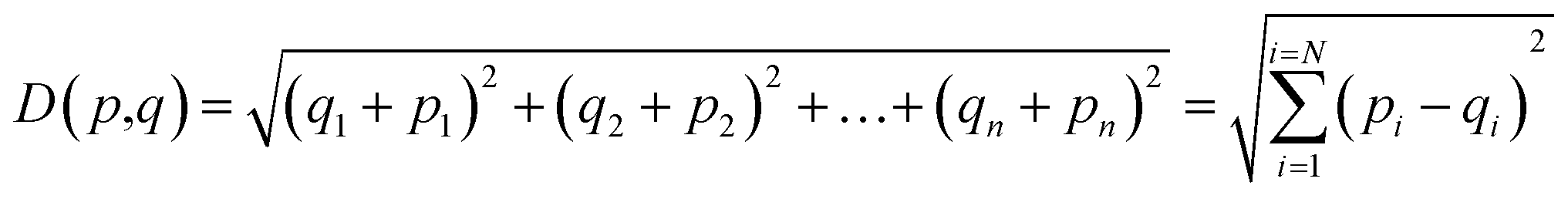 | (5) |
3.3.1.2.1 Data pre-processing for K-NN. The most prevalent method in the literature for analyzing Raman spectroscopy data is to use the peaks of the spectra. However, this method is very sensitive to noise in the data since a single noisy fluctuation in one of the points of the spectrum could change the result of the classification model. In this work, we introduce a novel method for analyzing Raman spectral data for cancer diagnosis by using the whole spectrum. As we will discuss in the results section, this method outperforms our decision tree algorithm which uses only the peaks of Raman spectral data. This is in part because we are extracting more information from the spectra and this extracted information is more robust to noise in the experimental setup.
For measurement s of patient i for biomarker b, our Raman spectra Rbi,s is a vector of 1783 intensities. This 1783-dimensional vector could be regarded as a point in a 1783-dimensional space. Therefore, we can define a similarity metric for the spectral data of a patient based on the Euclidian distance between the vectors of specific biomarkers. In addition, in order to use the entire data for all the biomarkers for each patient, we can create a large vector by appending all the vectors corresponding to different biomarkers and creating a larger vector.
| Ri,s = [RCA19-9i,s,RMUC4i,s,RMesothelini,s,RHE4i,s,RMMP7i,s] | (6) |
Given this high dimensional vector which contains the whole information of all the Raman spectral data for all biomarkers for a sample of a patient, first, we calculate the Euclidean distance between this new sample and the rest of the previously known training dataset. We then create a list containing all the distances:
| Distances = [D(Rtest,R1,1) D(Rtest,R1,1) … D(Rtest,Ri,s) … D(Rtest,Ri,s) … D(Rtest,Rn,10)] | (7) |
 | (8) |
 | (9) |
 | (10) |
3.3.3.1 Peak-value analysis. Classification trees are used to analyze the peak-value dataset of Raman shift measurements. Since the size of the dataset is limited, a specific test set is not held out to evaluate the performance of the classification. Instead, five-fold cross-validation is utilized to estimate the generalization error, in which the dataset is split into five equal subsets. Four subsets are used to train the model, and the other held-out subset is used to test the performance of the trained model. This train-test approach is performed five times, and in each test, one subset is held out. The outcome of these five tests for the sensitivity and specificity of the model are averaged and reported as the performance of the model. In order to avoid over-fitting, the depth of trees is limited to two.
The performance of the classification trees with 5-fold cross-validation with depth = 2 for an increasing number of biomarkers are presented in Table 2. The sensitivity and specificity for each panel of normal adults, pancreatic cancer patients, pancreatitis patients, and ovarian cancer patients in the table demonstrate that the accuracy of the early cancer perdition is improved by employing multiplex biomarkers.
| Biomarker(s) | Normal | Pancreatic cancer | Pancreatitis | Ovarian cancer | ||||
|---|---|---|---|---|---|---|---|---|
| Specificity | Sensitivity | Specificity | Sensitivity | Specificity | Sensitivity | Specificity | Sensitivity | |
| CA19-9 | 1 | 0.8 | 0.73 | 0.2 | 0.87 | 0.4 | 0.8 | 0.8 |
| CA19-9 + HE4 | 1 | 0.8 | 0.87 | 0.8 | 0.73 | 0.6 | 0.93 | 0.4 |
| CA19-9 + HE4 + mesothelin | 0.67 | 0.8 | 0.87 | 0.2 | 0.93 | 0.6 | 1 | 0.8 |
| CA19-9 + HE4 + mesothelin + MMP7 | 0.93 | 0.8 | 0.87 | 1 | 0.93 | 0.4 | 0.93 | 0.8 |
| CA19-9 + HE4 + mesothelin + MMP7 + MUC4 | 1 | 0.8 | 0.93 | 0.8 | 0.93 | 1 | 0.93 | 0.8 |
Finally, we used the whole dataset to train the classification tree shown in Fig. 6. This plot shows that the most important biomarkers in diagnosis are HE4, CA19-9, and MUC4, as expected. Note that the whole dataset is used to train this model. Therefore, the same data cannot be used to evaluate the performance of the model. It could be used to predict the healthiness of future patients.
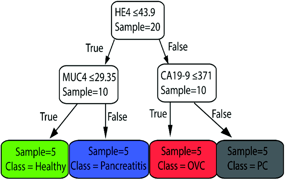 | ||
| Fig. 6 The classification tree trained with whole dataset of peak-value Raman shifts with depth = 2. This shows that the most important biomarkers in diagnosis are HE4, CA19-9, and MUC4. | ||
3.3.3.2 Full spectrum analysis. In order to achieve better accuracy, we have applied K-NN classifier with k = 5, which employs the full spectrum of all biomarkers. The whole dataset includes 200 vectors Ri,s of the format in eqn (6), which is randomly splitted in 20% for training data Rtraini,s and 80% for test data Rtesti,s. Using this setup, we achieved sensitivity of 86%, specificity 93%, and accuracy of 91% to predict the class of each measurement Rtesti,s in the test data. If we use the majority vote of the 5 measurements to diagnose the patient, the prediction would always be correct. Since the dataset size is limited, we cannot compute a more accurate estimation of the test error for this classifier.
The general setting of a K-NN classifier is very hard to visualize due to the high number of dimensions in the algorithm. In order to visualize how our K-NN algorithm works, we simplify our model to only two biomarkers. Fig. 7 depicts the scatter plot of the distance of a sample test data-point from all other data-points in the training set. The x-axis denotes the distance between the test data-point and all the training set data-points for the HE4 biomarker, D(RHE4test,RHE4train). The Y-axis denotes the distance between the test data-point and all the training set data-points for the CA19-9 biomarker, D(RCA19-9test,RCA19-9train). The point (0,0) in the plot, which is not shown, is where the test data-point resides. This is because the test data-point is regarded as the center for calculating all the corresponding distances. As it can be seen in the Fig. 7, all 5-nearest neighbors of the test patient's data points are diagnosed as PC. Therefore, we conclude that the unknown data point should be diagnosed as PC, which is a correct diagnosis for the test sample.
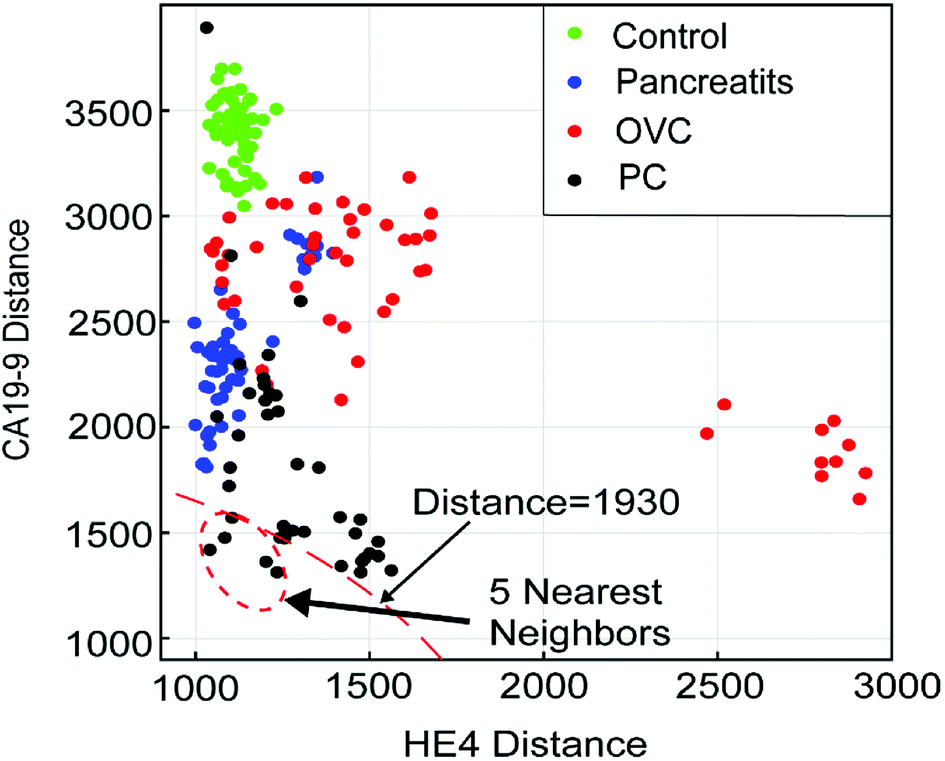 | ||
| Fig. 7 Scatter plot of the distance of a sample test data-point from all other data-points in the training set. In this case k in our K-NN algorithm is set to 5. The point (0,0), which is not shown, is where the test point resides. Looking at the 5-nearest neighbours, one quickly concludes that the test sample should be diagnosed as PC, which in this case is a correct diagnosis. | ||
In our case, we can clearly observe that when we translate our problem into K-NN, a small sample of our small dataset encapsulates lots of information about the spatial patterns between different classes. This means that there is a clear spatial separation between different classes in the defined high-dimensional space. In addition, it is worth noting that the smallness of our dataset is a limitation to any statistical analysis technique. Thus, we need to assess different statistical techniques with respect to their robustness. As mentioned earlier, using the smallest subset of our data (20%) as the training set for our K-NN model yields very accurate results which shows its robustness to the size of the training set. In our future work, we plan to increase the size of our dataset and perform state of the art machine learning techniques such as deep neural networks for statistical analysis.
In order to evaluate the effectiveness of adding new biomarkers to our classification problem, we make use of a conventional machine learning concept called Receiver Operating Characteristic (ROC) curve. In a ROC curve, true positive rate (TPR) is plotted against the false positive rate (FPR) at various threshold settings. The trained machine learning classifier outputs the probability that a given test sample is positive. To plot the ROC curve, we start by sorting all the test samples based on the predicted probability of being a positive sample. We then decrease the threshold gradually from 1 until it is equal to the highest probability and see if the corresponding sample test is a true positive or a false positive. If we have a true positive/false positive for our first sample, we draw a unit vertical/horizontal line starting from the point (0,0). We then continue decreasing the threshold to arrive at the next sample in our sorted list and continue to draw vertical/horizontal unit length lines for true positives/false positive. It has been shown that the area under the ROC curve (AUC) is equal to the probability that a classifier will rank a randomly chosen positive instance higher than a randomly chosen negative one (assuming 'positive' ranks higher than 'negative'). AUC is a standard metric for evaluating machine learning classifiers. A perfect predictor has AUC of 1. On the other hand, a random prediction model gives us AUC of 0.5. To this end, the K-NN model is trained with 80 percent of the data using K = 3 and tested with the other 20 percent of the data. This arrangement is chosen to demonstrate the effect of biomarkers more clearly. Fig. 8 shows the ROC curve for various combinations of biomarkers. As it can be seen in the Fig. 8, adding biomarkers significantly increases our prediction accuracy.
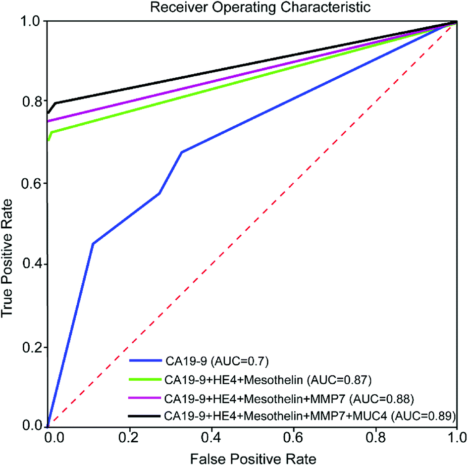 | ||
| Fig. 8 ROC curve for various combinations of biomarkers for the k-nearest neighbour model with k = 3 and 80 percent of the data as the training set and 20 percent as the test set. | ||
4. Conclusions
This study demonstrated that microfluidic assay significantly reduced about 50% of the Raman signal measurement variation as compared to conventional assays. Multiplex detection of five biomarkers which elevate in both PC and ovarian cancer was accomplished with microfluidic SERS-based immunoassay approach.We employed decision tree classification and nearest neighbor method to evaluate the importance of different biomarkers and estimate the specificity and accuracy of the prediction. The result from data analysis demonstrated that multiplex detection of protein biomarkers (CA19-9, HE4, MUC4, MMP7, and mesothelin) in cancer patients and diseases with similar protein biomarkers significantly increased specificity and prediction accuracy. It is also observed that HE4 and MUC4 biomarkers improved the specificity of diagnosis, in addition to CA19-9 biomarker.
Conflicts of interest
There are no conflicts to declare.Acknowledgements
This work is supported by the IALS Seed Grant from the University of Massachusetts Amherst.References
- S. T. Chari, K. Kelly and M. A. Hollingsworth, et al., Early detection of sporadic pancreatic cancer: summative review, Pancreas, 2015, 44(5), 693–712 CrossRef PubMed.
- I. Bozic, J. G. Reiter and B. Allen, et al., Evolutionary dynamics of cancer in response to targeted combination therapy, eLife, 2013, 2, e00747 CrossRef PubMed.
- V. M. Kim and N. Ahuja, Early detection of pancreatic cancer, Chin. J. Cancer Res., 2015, 27(4), 321–331 CAS.
- J. D. Cohen, L. Li and Y. Wang, et al., Detection and localization of surgically resectable cancers with a multi-analyte blood test, Science, 2018, eaar3247 Search PubMed.
- J. D. Cohen, A. A. Javed and C. Thoburn, et al., Combined circulating tumor DNA and protein biomarker-based liquid biopsy for the earlier detection of pancreatic cancers, Proc. Natl. Acad. Sci. U. S. A., 2017, 114(38), 10202–10207 CrossRef CAS PubMed.
- K. Mäbert, M. Cojoc, C. Peitzsch, I. Kurth, S. Souchelnytskyi and A. Dubrovska, Cancer biomarker discovery: current status and future perspectives, Int. J. Radiat. Biol., 2014, 90(8), 659–677 CrossRef PubMed.
- F. Legrand, D. Berrebi and N. Houhou, et al., Early diagnosis of adenovirus infection and treatment with cidofovir after bone marrow transplantation in children, Bone Marrow Transplant., 2001, 27(6), 621 CrossRef CAS PubMed.
- E. F. Patz Jr, M. J. Campa, E. B. Gottlin, I. Kusmartseva, X. R. Guan and J. E. Herndon, Panel of serum biomarkers for the diagnosis of lung cancer, J. Clin. Oncol., 2007, 25(35), 5578–5583 CrossRef PubMed.
- D. E. Misek and E. H. Kim, Protein biomarkers for the early detection of breast cancer, Int. J. Proteomics, 2011, 2011, 343582 Search PubMed.
- G. Mor, I. Visintin and Y. Lai, et al., Serum protein markers for early detection of ovarian cancer, Proc. Natl. Acad. Sci. U. S. A., 2005, 102(21), 7677–7682 CrossRef CAS PubMed.
- M. J. Engelen, H. W. de Bruijn and H. Hollema, et al., Serum CA 125, carcinoembryonic antigen, and CA 19-9 as tumor markers in borderline ovarian tumors, Gynecol. Oncol., 2000, 78(1), 16–20 CrossRef CAS PubMed.
- M. Duffy, C. Sturgeon and R. Lamerz, et al., Tumor markers in pancreatic cancer: a european group on tumor markers (EGTM) status report, Ann. Oncol., 2009, 21(3), 441–447 CrossRef PubMed.
- R. G. Moore, D. S. McMeekin and A. K. Brown, et al., A novel multiple marker bioassay utilizing HE4 and CA125 for the prediction of ovarian cancer in patients with a pelvic mass, Gynecol. Oncol., 2009, 112(1), 40–46 CrossRef CAS PubMed.
- A. R. Simmons, K. Baggerly and R. C. Bast Jr, The emerging role of HE4 in the evaluation of epithelial ovarian and endometrial carcinomas, Oncology, 2013, 27(6), 548–556 Search PubMed.
- R. L. O'Neal, K. T. Nam and B. J. LaFleur, et al., Human epididymis protein 4 is up-regulated in gastric and pancreatic adenocarcinomas, Hum. Pathol., 2013, 44(5), 734–742 CrossRef PubMed.
- T. Huang, S. Jiang and L. Qin, et al., Expression and diagnostic value of HE4 in pancreatic adenocarcinoma, Int. J. Mol. Sci., 2015, 16(2), 2956–2970 CrossRef CAS PubMed.
- B. McKINNON, M. D. Mueller, K. Nirgianakis and N. A. Bersinger, Comparison of ovarian cancer markers in endometriosis favours HE4 over CA125, Mol. Med. Rep., 2015, 12(4), 5179–5184 CrossRef CAS PubMed.
- P. Lamy, C. Plassot and J. Pujol, Serum HE4: an independent prognostic factor in non-small cell lung cancer, PLoS One, 2015, 10(6), e0128836 CrossRef PubMed.
- Q. F. Tang, Z. W. Zhou, H. B. Ji, W. H. Pan and M. Z. Sun, Value of serum marker HE4 in pulmonary carcinoma diagnosis, Int. J. Clin. Exp. Med., 2015, 8(10), 19014–19021 CAS.
- K. F. Kuhlmann, J. W. van Till and M. A. Boermeester, et al., Evaluation of matrix metalloproteinase 7 in plasma and pancreatic juice as a biomarker for pancreatic cancer, Cancer Epidemiol., Biomarkers Prev., 2007, 16(5), 886–891 CrossRef CAS PubMed.
- C. L. Wilson, K. J. Heppner, P. A. Labosky, B. L. Hogan and L. M. Matrisian, Intestinal tumorigenesis is suppressed in mice lacking the metalloproteinase matrilysin, Proc. Natl. Acad. Sci. U. S. A., 1997, 94(4), 1402–1407 CrossRef CAS.
- H. Yamamoto, F. Itoh and S. Iku, et al., Expression of matrix metalloproteinases and tissue inhibitors of metalloproteinases in human pancreatic adenocarcinomas: clinicopathologic and prognostic significance of matrilysin expression, J. Clin. Oncol., 2001, 19(4), 1118–1127 CrossRef CAS PubMed.
- S. Carrara, M. G. Cangi and P. G. Arcidiacono, et al., Mucin expression pattern in pancreatic diseases: findings from EUS-guided fine-needle aspiration biopsies, Am. J. Gastroenterol., 2011, 106(7), 1359–1363 CrossRef CAS PubMed.
- A. Horn, S. Chakraborty and P. Dey, et al., Immunocytochemistry for MUC4 and MUC16 is a useful adjunct in the diagnosis of pancreatic adenocarcinoma on fine-needle aspiration cytology, Arch. Pathol. Lab. Med., 2013, 137(4), 546–551 CrossRef CAS PubMed.
- P. Argani, C. Iacobuzio-Donahue and B. Ryu, et al., Mesothelin is overexpressed in the vast majority of ductal adenocarcinomas of the pancreas: identification of a new pancreatic cancer marker by serial analysis of gene expression (SAGE), Clin. Cancer Res., 2001, 7(12), 3862–3868 CAS.
- R. Hassan, Z. G. Laszik, M. Lerner, M. Raffeld, R. Postier and D. Brackett, Mesothelin is overexpressed in pancreaticobiliary adenocarcinomas but not in normal pancreas and chronic pancreatitis, Am. J. Clin. Pathol., 2005, 124(6), 838–845 CrossRef CAS PubMed.
- L. J. Havrilesky, C. M. Whitehead and J. M. Rubatt, et al., Evaluation of biomarker panels for early stage ovarian cancer detection and monitoring for disease recurrence, Gynecol. Oncol., 2008, 110(3), 374–382 CrossRef CAS PubMed.
- S. C. Chauhan, A. P. Singh and F. Ruiz, et al., Aberrant expression of MUC4 in ovarian carcinoma: diagnostic significance alone and in combination with MUC1 and MUC16 (CA125), Mod. Pathol., 2006, 19(10), 1386 CrossRef CAS PubMed.
- R. Hassan, A. T. Remaley and M. L. Sampson, et al., Detection and quantitation of serum mesothelin, a tumor marker for patients with mesothelioma and ovarian cancer, Clin. Cancer Res., 2006, 12(2), 447–453 CrossRef CAS PubMed.
- M. K. Beeharry, W. T. Liu, M. Yan and Z. G. Zhu, New blood markers detection technology: a leap in the diagnosis of gastric cancer, World J. Gastroenterol., 2016, 22(3), 1202–1212 CrossRef CAS PubMed.
- S. K. Huang and D. S. Hoon, Liquid biopsy utility for the surveillance of cutaneous malignant melanoma patients, Mol. Oncol., 2016, 10(3), 450–463 CrossRef CAS PubMed.
- N. Banaei, A. Foley, J. M. Houghton, Y. Sun and B. Kim, Multiplex detection of pancreatic cancer biomarkers using a SERS-based immunoassay, Nanotechnology, 2017, 28(45), 455101 CrossRef PubMed.
- S. Schlücker, Surface-enhanced Raman spectroscopy: concepts and chemical applications, Angew. Chem., Int. Ed., 2014, 53(19), 4756–4795 CrossRef PubMed.
- U. Dinish, G. Balasundaram, Y. T. Chang and M. Olivo, Sensitive multiplex detection of serological liver cancer biomarkers using SERS-active photonic crystal fiber probe, J. Biophotonics, 2014, 7(11–12), 956–965 CrossRef CAS PubMed.
- C. L. Zavaleta, B. R. Smith and I. Walton, et al., Multiplexed imaging of surface enhanced Raman scattering nanotags in living mice using noninvasive Raman spectroscopy, Proc. Natl. Acad. Sci. U. S. A., 2009, 106(32), 13511–13516 CrossRef CAS PubMed.
- N. Guarrotxena, B. Liu, L. Fabris and G. C. Bazan, Antitags: nanostructured tools for developing SERS-based ELISA analogs, Adv. Mater., 2010, 22(44), 4954–4958 CrossRef CAS PubMed.
- S. Feng, R. Chen and J. Lin, et al., Nasopharyngeal cancer detection based on blood plasma surface-enhanced Raman spectroscopy and multivariate analysis, Biosens. Bioelectron., 2010, 25(11), 2414–2419 CrossRef CAS PubMed.
- D. Lin, S. Feng and J. Pan, et al., Colorectal cancer detection by gold nanoparticle based surface-enhanced Raman spectroscopy of blood serum and statistical analysis, Opt. Express, 2011, 19(14), 13565–13577 CrossRef CAS PubMed.
- M. Lee, K. Lee, K. H. Kim, K. W. Oh and J. Choo, SERS-based immunoassay using a gold array-embedded gradient microfluidic chip, Lab Chip, 2012, 12(19), 3720–3727 RSC.
- R. Gao, J. Ko and K. Cha, et al., Fast and sensitive detection of an anthrax biomarker using SERS-based solenoid microfluidic sensor, Biosens. Bioelectron., 2015, 72, 230–236 CrossRef CAS PubMed.
- G. Wang, H. Park, R. J. Lipert and M. D. Porter, Mixed monolayers on gold nanoparticle labels for multiplexed surface-enhanced Raman scattering based immunoassays, Anal. Chem., 2009, 81(23), 9643–9650 CrossRef CAS PubMed.
- L. Breiman, Classification and regression trees, Routledge, 2017 Search PubMed.
- K. S. Kim, H. H. Choi, C. S. Moon and C. W. Mun, Comparison of k-nearest neighbor, quadratic discriminant and linear discriminant analysis in classification of electromyogram signals based on the wrist-motion directions, Curr. Appl. Phys., 2011, 11(3), 740–745 CrossRef.
- S. Tayeb, M. Pirouz and J. Sun, et al., Toward predicting medical conditions using k-nearest neighbors, 2017, pp. 3897–3903 Search PubMed.
- V. Prasath, H. A. A. Alfeilat, O. Lasassmeh and A. Hassanat, Distance and similarity measures effect on the performance of K-nearest neighbor classifier-a review, arXiv:1708.04321, 2017.
- D. J. Hand, Principles of data mining, Drug Saf., 2007, 30(7), 621–622 CrossRef PubMed.
- F. Pedregosa, G. Varoquaux and A. Gramfort, et al., Scikit-learn: machine learning in python, J. Mach. Learn. Res., 2011, 12, 2825–2830 Search PubMed.
Footnote |
| † Electronic supplementary information (ESI) available. See DOI: 10.1039/c8ra08930b |
| This journal is © The Royal Society of Chemistry 2019 |