Characteristics of water quality and bacterial communities in three water supply pipelines

Abstract

Many cities in China have implemented urban water supply pipe network renovation projects; however, at the beginning of new pipeline replacements, customers often complain about water quality problems, such as red water, odour and other water quality problems. To overcome these frequent water quality problems, this study selected a commonly used ductile cast iron (DCI) pipe, stainless steel (SS) pipe and high-density polyethylene (HDPE) pipe for laboratory simulations of the water quality regularity of new pipes, the variations in pipe inner walls, and the presence of microbial communities. Based on the research results, combined with actual water sample analysis, the stabilisation time of the interaction between the tubings inner walls and bulk water was determined, to allow pipeline cleaning and water quality maintenance. The results showed that the water quality change in the DCI was the most significant, while the SS and the HDPE pipes showed consistent changes with severe initial deterioration, then later stabilisation to meet the required standard. The DCI inner wall changed from a loose porous particle shape to a relatively dense and irregular three-dimensional shape, with the constituent elements mainly being O and Ca. The SS inner wall had a uniform structure in the early stage, but are obvious spherical balls of different sizes formed later, with the elemental composition here mainly being C and O. The HDPE inner wall was smooth and had small perforations in the early stage, while the perforation in the middle and late stages increased to become rough and scale-like at a much later stage. The proportion of Proteobacteria in effluents (72.82% to 86.87%) was significantly increased compared with the influent (48.45%), while the proportion of Proteobacteria (86.87%) in the DCI was significantly higher than in the SS (74.28%) and HDPE pipes (81.68%). Moreover, compared with the influent (23.33%), the Bacteroidetes (2.79% to 3.32%) levels in the effluents were significantly reduced, indicating that the pipe material affects the microbial abundance in water.

---

1. Introduction

Drinking water distribution system (DWDS) is buried underground and involve complicated networked connections. In addition, such systems involve a huge tubular reactor, which consists of different materials and different pipe diameters.^1–3 The treated drinking water (TDW) may undergo physical, chemical and biological reactions in the pipelines through coagulation, sedimentation, filtration and disinfection processes conducted in the waterworks, and these reactions may vary as the seasons change and the tubing material varies.^4–6 In addition, the DWDS serves as a huge information channel, and the TDW can be regarded as a kind of carrier. The TDW enters the DWDS and carries much information related to the water quality, such as turbidity, colour, residual chlorine, total bacteria, assimilable organic carbon (AOC) and disinfection by-products.⁷ As the bulk water flow rate and hydraulic retention time (HRT) change, also extending the interaction time between the pipeline inner walls and bulk water, the information also changes accordingly as water is redistributed and recombined within the pipeline.^8,9

In an urban DWDS, steel and cast iron pipes have been used for centuries.^10–13 In China, more than 90% of the water supply pipelines are made of cast iron or steel. New DWDSs under construction are also mainly made of metal pipes, with a utilisation rate of 86%.¹⁴ However, metals are easily corroded in media such as drinking water containing various electrolytes and microorganisms. Corrosion can release some elements that make up the DWDS into the TDW, changing various indicators of the TDW and resulting in secondary pollution.^15–17 Corrosion of the water supply pipeline can not only lead to deterioration of the indicators (such as colour, turbidity, bacteria, iron and manganese, organic matter and toxic heavy metal content) but also cause the pipeline wall to become thin and rough and increase the energy consumption required for water transportation, eventually leading to leakage of water through the pipe, and shortening the service life of the pipelines.

According to TDW samples in one study taken from Chicago in 1968 compared to water samples taken after passing through a DWDS, the results of water quality testing showed that the concentrations of Cd, Cr, Co, Cu, Fe, Pb, Mn, Ni, Ag, Zn and other elements had increased by 15% to 67% in the water samples. Pipeline corrosion can also increase the consumption of disinfectants and reduce residual chlorine levels in the DWDS. The maximum corrosion rate of a low-carbon steel water supply pipe in the USA is (7.62 to 12.7) × 10⁻² mm a⁻¹.¹⁸ For free chlorine disinfected drinking water, when the corrosion rate is greater than 0.0254 mm a⁻¹, the disinfection effect will be lost. At the same time, when the water source is replaced, the pipeline corrosion may cause serious coloured water problems. For example, there have been red water incidents in many areas in the US in areas such as Southern California, Tucson, Arizona and Tampa, Florida that have attempted to substitute the water supply source from ground water with surface water, but the results showed that the release of iron ions forms a large amount of sediment due to the interaction of the change in the quality of the raw water and the corrosion of the pipeline, resulting in red water.^19–22 In China, at the end of September 2008, raw water from four reservoirs in Hebei Province arriving in Beijing via the South-to-North water transfer open channel was used to replace the original groundwater source.^23–25 The result also led to the emergence of red water in some areas. These were because of pipeline corrosion releasing iron to form ferric hydroxide in the drinking water.²⁶

In a DWDS, the growth of microbes is inevitable. Previous researchers have investigated the corrosion of old tubing by microorganisms in various systems. The growth and reproduction of microorganisms cause corrosion and a deterioration in the water quality in the DWDS, caused by biological instability.⁶ At present, the effluent from waterworks has been chlorinated and disinfected, but there is still a small amount of bacteria therein, and further, the bacteria that are not killed by chlorine tend to be more tenacious.^27,28 Moreover, organic matter is present in the TDW, so that the bacteria in the water use these organic nutrients for regrowth and reproduction.^29,30 The self-repairing growth of bacteria that have not been killed after chlorine disinfection and the entry of external bacteria into the pipeline are factors leading to bacterial growth, whereas the tube wall roughness, boundary layer effect, laminar flow zone, sedimentation of suspended matter and colloidal matter, corrosion, rust, scale formed by calcium and magnesium, etc. provide a base for bacterial reproduction.³¹ However, few researchers have studied the microbial characteristics of new pipes in the DWDS.

In 1999, the American Water Works Association (AWWA) estimated that in the next 20 years, water companies would spend $325 billion to upgrade urban DWDSs in the USA alone.¹⁰ In 2002, the Water Supplies Department of Hong Kong embarked on a large-scale programme to replace 60% of the water mains throughout the territory in twenty years so as to minimise the inconvenience caused by main breaks.^32,33 In recent years, large cities in mainland China have gradually begun to update their urban DWDSs to solve the various existing water supply problems and to further improve the water quality delivered at the customers' tap; however, after new pipelines are first used, the tubing inner wall and the bulk water needed a period of adaptation, and consumers complained of many problems such as coloured or odiferous tap water. Consequently, a study of the water quality changes, the characteristics of the tubing inner walls and the water microbial community characteristics at the beginning of a new pipeline is necessary and vital. Unfortunately, there is no literature report on this area.

To improve drinking water quality, and solve the secondary pollution and red water problems facing Shenzhen, Guangdong Province, China, Shenzhen officially launched a high-quality drinking water project in 2013, whereby the old DWDSs of the residential area were replaced with new ones, with a plan to complete all tasks by 2020. At present, the main pipes used in the pipeline renovation process in the city include ductile cast iron (DCI) pipes, stainless steel (SS) pipes and high-density polyethylene (HDPE) pipes. This study mainly simulates the effects of three pipelines on drinking water in the laboratory, combined with field water sample collection and analysis in Yantian District, Shenzhen (ESI 2†). The study explored the adaptation period of different tubing materials and determined the water quality stabilisation time in different new tubing materials, with an aim to provide theoretical support for the implementation of water quality guarantee measures in the initial stage of an urban DWDS.

2. Materials and methods

2.1 Laboratory-scale reactor operation

The experiment used newly-purchased DCI (which were cement mortar lined), SS, and HDPE pipes of 150 mm diameter, that were machined into 150 mm long test pipe sections. Each pipe section was sealed with epoxy resin to prevent contact with water. Before testing, the pipe sections were cleaned with alcohol for removal of oil, and then the pipe sections were cleaned with TDW and rinsed slowly for 30 min, after which the TDW was leak-tested and the pipe section stabilised for 12 h. After pre-treatment, each pipe section was fixed in the annular reactor (AR), then the TDW was added, the bulk water was stirred using a polyethylene stirring blade, and the flow condition of the longitudinal water flow in the actual DWDS was simulated by lateral circulation flow to ensure a certain shearing force in the pipe sections.^8,34,35

The angular velocity of the AR was 250 rpm, which equated with a shearing velocity of about 0.2 m s⁻¹ in the pipe.³⁶ Thereby, the water quality changes generated after long-term contact between the TDW and the pipe section inner wall were simulated in the shorter pipe sections. The AR test system is shown in Fig. S1.† The inner wall material of each tubing sample was cut into several pieces, each measuring 10 mm × 10 mm. The incisions were wrapped with epoxy resin and placed in the bottom of each AR test system. Two pieces were taken before operation and again on the 14^th and 25^th days after operation, with variations on the inner wall of the different material pipes characterised by scanning electron microscopy (SEM) and energy dispersive spectroscopy (EDS). At the end of the operation, the microbial communities of influent and effluent water were analysed.

There are two ways to select an HRT: the one is trying to simulate the actual hydraulic retention time; the other one due to the new pipeline materialisation reaction is slow, for the rapid identification problem, the simulation is carried out under the most unfavourable conditions.⁸ Based on the hydraulic model, the HRT was calculated. The HRT under normal conditions was 8 to 12 h, and 27 h under the most extreme conditions. At the same time, the statistics on user complaints showed that the water quality problems were the most serious after 20 d to 30 d of new pipeline operation; therefore, the study selected the hydraulic conditions with an HRT of 24 h and a running time of 25 d. Water was discharged completely from the AR systems every day and fresh TDW was then fed into the systems.

2.2 Test water and water quality analysis

The influent of the ARs was fresh TDW from the waterworks in Shenzhen, China. The tap of the influent was opened for 30 min before the influent was sampled daily. The water quality was deemed stable. The main water quality parameters of the influent, the “Standards for Drinking Water Quality” (GB5746-2006) (National Standard), and the “Water Quality Target Items and Limits of Drinking Water in Shenzhen” are shown in Table S1.†

The quality parameters of the influent and effluent were analysed on a daily basis. The monitored water quality parameters and test methods are summarised in Table S2.†

2.3 Microbial sample preparation, DNA extraction and PCR amplification

On the 25th day after the AR test systems were first operated, the influent and effluents from each AR were collected. The biological samples of the influent and effluents were enriched by 0.22 μm filter membrane (Millipore), with the condition that the amount of water filtered should be no less than 5 L for assurance of the biomass. The enriched biomass was stored in sterilised 50 mL centrifuge tubes at −80 °C for further processing.^36,37

The DNA of the samples was extracted by the CTAB method, and then the purity and concentration of the DNA were detected by agarose gel electrophoresis. The appropriate amount of the sample was taken in a centrifuge tube, and the sample was diluted to 1 ng μL⁻¹ with sterile water. Using diluted genomic DNA as a template, according to the selection of sequencing regions to ensure amplification efficiency and accuracy, the PCR was carried using Phusion® High-Fidelity PCR Master Mix with GC Buffer (New England Biolabs) and high-efficiency, high-fidelity enzymes that were specific primers with barcode.

The PCR amplification used the V4 variable region amplification primers, with the sequences: barcode-515F (5′-GTGYCAGCMGCCGCGGTAA-3′) and 806R (5′-GGACTACNVGGGTWTCTAA-3′).^38–40

2.4 Product purification, library preparation and inspection and sequencing on HiSeq

The PCR product was detected by electrophoresis using a 2% agarose gel. The samples were mixed thoroughly according to the concentration of the PCR product, and the PCR product was detected by 2% agarose gel electrophoresis. The target strip was provided by Qiagen. The glue recovery kit was used to recover the product.

The library was constructed using the TruSeq® DNA PCR-Free Sample Preparation Kit. The constructed library was quantified by Qubit and Q-PCR. After the library was qualified, it was sequenced using HiSeq2500 PE250.

3. Results and discussion

3.1 Water quality analysis

Water quality variations of the influent and effluents are shown in Fig. 1 and S2.† Fig. 1 (line chart) shows the changes in water quality index with the increase in running time within 25 days; moreover, Fig. S2† (box-plot) shows the overall situation of the water quality index over these 25 days.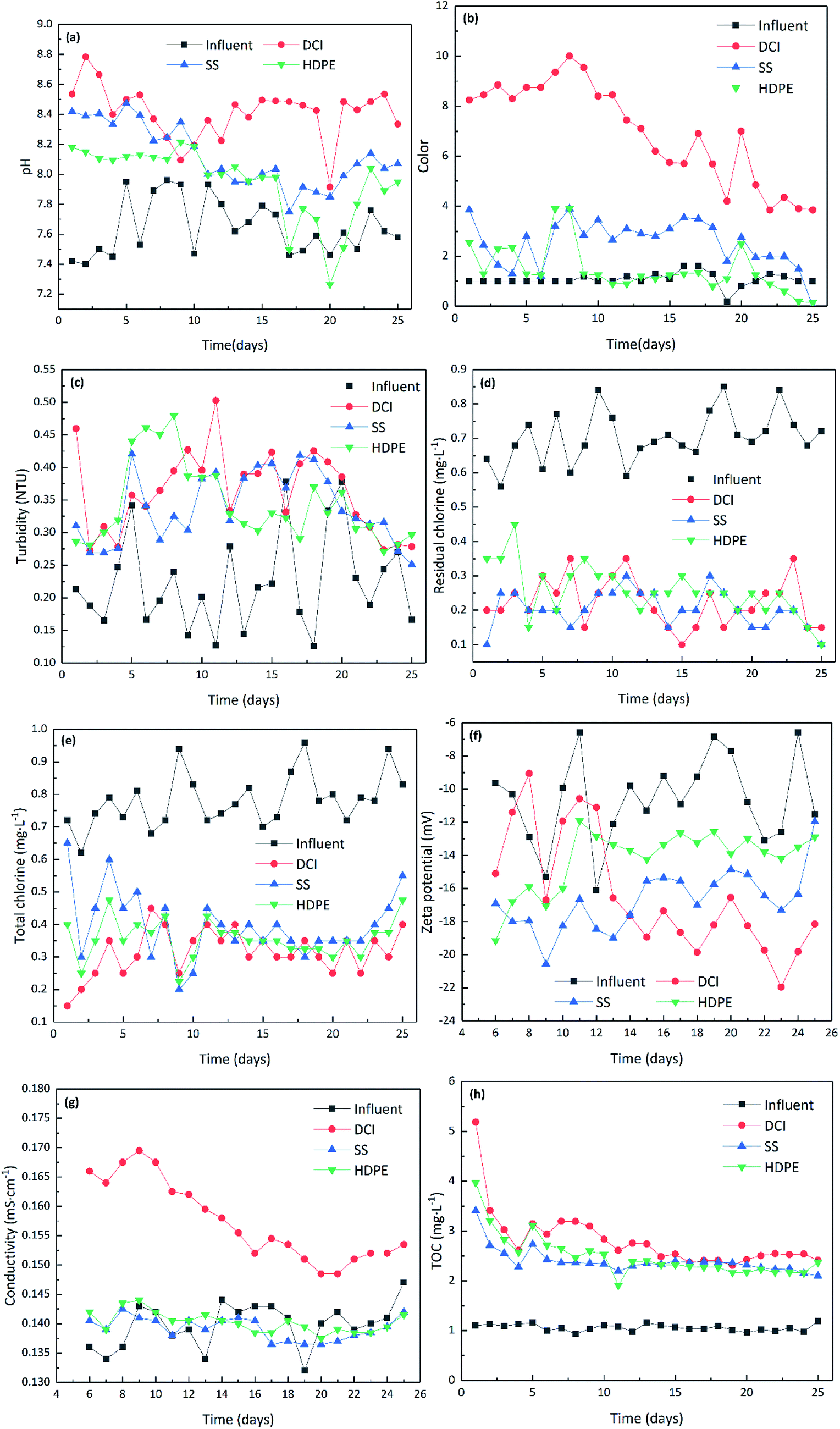

Fig. 1 Variation of water quality in AR systems.

3.1.1 pH. Due to the different materials, there were significant differences in the effluent pH of the three tubings. As shown in Fig. 1(a) and S2(a),† the effluent pH values of the three tubings were always significantly higher than those of the influent, with that of the DCI pipe being the most significant. As shown in Fig. 1(a), when the pH of the influent was between 7.5 and 8.0, the pH of the effluents increased during operation, with the pH of the DCI pipe effluent always higher than 8.0, up to a highest pH of 8.8, while the pH of the SS and HDPE tubes was always less than 8.5. In the later stages of operation, the pH of the SS effluent was maintained at about 8.0, and the pH of HDPE was different from that of the influent. The laboratory simulation results are basically consistent with the actual water sample analysis results (ESI 2†). Although the lining of the DCI can protect the iron from corrosion, the dissolution of alkaline substances in the lining cause the pH to rise.^28,41,42 Slaats et al. found that the corrosion of the inner walls of cement-containing pipes involves the leaching of hydroxides, causing pH changes and resulting in scaling in the water mains and domestic installations.⁴³ Bonds et al. reported that cement linings prevent tuberculation by creating a high pH at the pipe wall; moreover leachates from the uncoated cement lining can cause an undesirable rise in the pH of the water, particularly under low flow conditions in small-diameter pipes.⁴⁴ Due to the long HRT of this test (24 h), the dissolution of the DCI pipe resulted in a significant increase in pH.⁴³

3.1.2 Colour and turbidity. The variation in colour and turbidity of the influent and effluent are shown in Fig. 1 and S2.† The laboratory simulation results are basically consistent with the actual water sample analysis results (ESI 2†).

As shown in Fig. 1(b) and S2(b),† during operation, the colour increase of the DCI pipe was significant, always higher than that of the SS and HDPE pipes, such that the colour reached 10, and the colour of effluent in the SS and HDPE pipes also increased; however, the colour was maintained at within 4, and there was not much difference between the late effluent and the influent. Previous studies have found that the colour of the DCI pipe can significantly increase, mainly due to the dissolution of ferric ions contained in the iron-aluminum tetracalcium (4CaO·Al₂O₃·Fe₂O₃) in the cement mortar lining.^41,42 Li et al. reported that the elevated pH is accompanied by high alkalinity, whereby CO₃²⁻ in bulk water might react with the iron release to generate poorly settling substances, such as siderite (FeCO₃), resulting in a rise in turbidity and colour.⁸

It can be seen from Fig. 1(c) and S2(c)† that, during operation, the turbidity of the effluent from the three tubings increased significantly. Among these, the HDPE pipe increased significantly in the first 10 days, and the effluent turbidity of the DCI pipe was unstable. Only the SS pipe remained at 0.35 NTU, and the turbidity of water from the latter three tubings was less than 0.3 NTU. During operation, the effluent turbidity of the three tubings were generally higher than the influent. The main reason for the turbidity characteristics of this kind of change may be due to the water being renewed every day, whereby the residual chlorine quickly kills the surviving microorganisms, making it difficult for the microorganisms to produce more extracellular secretions that can increase turbidity in the environment,⁴⁵ and the lining of the DCI pipe provides a haven for a small number of microorganisms. Also, the turbidity in the DCI pipe is more significant than that in the water from the SS and HDPE pipes. Simoes et al. reported that biofilm growth in DWDS contributes to the accumulation of inorganic particles, whereby any inorganic particle passing nearby (e.g. corrosion products, clays, sand) may be incorporated in the biofilms, in the distribution network, which are responsible for discoloured water and are a persistent cause of customer dissatisfaction.³¹

3.1.3 Residual chlorine and total chlorine. In the waterworks, liquid chlorine is used as the main disinfectant to maintain the disinfection effect in the DWDSs. The consumption of residual chlorine in the DWDSs is mainly reflected in two aspects: (1) it reacts with the reducing oxygen-consuming organic matter in the DWDS,^46–50 (2) it reacts with the corrosion scale or the biofilm on the pipe wall, and the tubing itself.^51–55 The pipe material is one of the main factors influencing residual chlorine decay.^54,56–58 Different tubing materials have certain effects on the residual chlorine degradation of water quality.^28,59 The laboratory simulation results are basically consistent with the changes of residual chlorine and total chlorine in the actual water sample analysis, but the values of residual chlorine and total chlorine in the actual sampling are significantly higher than in the experimental simulation results (ESI 2†). The reason for this may be due to the fact the experimental values were measured after a long hydraulic stay, with the water from the actual community passing throughout the whole night, and where customer use promotes the flow of water in the morning, thus supplementing the residual chlorine and total chlorine value of the water.

As shown in Fig. 1(d) and S2(d),† the trends in the consumption of residual chlorine in the three tubing sample materials are similar. These results showed that the residual chlorine decay intensity of the tubing samples in descending order was DCI, HDPE, and SS. However, chlorine decay experiments carried out by Zhang et al. showed the chlorine decay trend as SS, DCI, and polyethylene (PE) pipe, mainly because all their samples were 3 years old.⁵⁴ The trend in total chlorine is shown in Fig. 1(e) and S2(e).† The variation is similar to that of free residual chlorine. The total chlorine attenuation intensity of the tubings in descending order was: DCI, HDPE, and SS. This result is consistent with the conclusions of Zhong et al. with regard to the variation of residual chlorine.⁶⁰ The main reason for this is that the lining of the DCI has a large specific surface area, which provides a larger habitat for microorganisms.⁴¹ On the other hand, the inner wall of the SS pipe is smooth, and the microorganisms find it difficult to adhere to a large number of reproduction sites, while the HDPE pipe consumes a large amount of residual chlorine due to the inner wall being made of organic matter,⁹ which is consistent with previous research results.^61,62

3.1.4 Metal ions. This study monitored the levels of ferrous (Fe²⁺), ferric (Fe³⁺), and manganese (Mn), which can cause red water problems in the influent and effluents within 25 days. The results showed that the content of the three metal ions in the influent water was lower than the detection limit of the instrument. Similarly, the content of the three metal ions in the effluents within 25 days remained lower than the detection limit of the instrument (well below standard control limits). It can thus be seen that the tubing material contributes very little to the metal ions in bulk water in the early stages of the new pipeline operations. However, the variation of metal ions was detected in the actual water sample analysis (ESI 2†). All three metal ions showed a trend of increasing in the early stage and decreasing in the later stage.

3.1.5 Zeta potential and conductivity. The zeta potential is an important indicator characterising the stability of colloidal systems. If the particles carry a lot of negative or positive charges, it means that the absolute value of the zeta potential is very high, and the particles will repel each other to achieve stability in the whole system; otherwise, they will attract each other, making the whole system unstable.⁶³ In general, the higher the zeta potential, the more stable the dispersion of the particles. Further, the boundary between the dispersion stability of the particles in the aqueous phase is generally considered to be +30 mV or −30 mV, at greater than +30 mV, or at less than −30 mV, the dispersion is relatively stable. The zeta potential and conductivity of the actual water sample here were higher than the experimental simulation results (ESI 2†).

The zeta potentials were negative during the operation of the three tubing types in this research. Fig. 1(f) and S2(f)† show the zeta potential change. The zeta potential of the DCI pipe was gradually reduced from the initial −15.1 mV to −18 mV. The zeta potential of the SS pipe was relatively stable and was maintained at around −15 mV. The initial zeta potential of the HDPE pipe reached −19.1 mV, and this gradually increased and was maintained at −13 mV in the later stage. Previous studies have shown that under alkaline conditions, the zeta potential of the system is lower than that under acidic conditions, and the suspension system is more stable, which is consistent with the conclusions of this research. At the same time, studies have shown that the absolute value of the zeta potential and the content of the salt in the solution are related, so the dissolution of the lining of the DCI pipe is also one of the factors that cause a higher absolute value of the zeta potential.⁶⁴

The conductivity of drinking water refers to the ability of an aqueous solution to conduct electrical current, and is closely related to the mineral content of drinking water. The conductivity can be used to monitor changes in dissolved mineral concentrations in drinking water and to estimate the amount of ionic compounds in aqueous solutions. Most inorganic salts in water are in an ionic state and are good conductors of electricity. The conductivity of water is proportional to the concentration of electrolyte and is linearly related, whereby the lower the conductivity of water, the purer the water. Fig. 1(g) and S2(g)† show the change in conductivity of the three tubing types. The DCI pipe had a higher conductivity than the SS and HDPE pipes, while the water in the SS and HDPE pipes showed little difference to the influent conductivity.

3.1.6 TOC. TOC characterises the total organic carbon content in water and is a comprehensive indicator of organic pollution. During operation, a change in TOC can reflect the dissolution of organic matter in the tubing. Fig. 1(h) and S2(h)† show the TOC changes in the bulk water with different running times in different tubing samples. The TOC trends in the three tubing types were consistent: the initial stage was relatively high, while in the later stage, it gradually reduced and tended to be stable. The TOC of the actual water sample was lower than the experimental simulation results, which may be due to the same reason as that for the actual residual chlorine and total chlorine (ESI 2†).

According to the previous research, the reason for this is that the microbes rapidly multiply in the initial stage.^65–67 At the same time as the organic matter is consumed, the microorganisms that are killed and that have naturally died are released into the bulk water, so that the concentration of TOC increases. After the stabilisation period, the number of bacteria gradually decreases, and some organic material is consumed by the residual chlorine reaction, resulting in a decrease in the effluent TOC, but such that it remains higher than that in the influent. Deb et al. found that the dissolution of humus-like organic matter (such as humic acid and fulvic acid) in the sand lining of the DCI pipe cement mortar is also one of the factors that increases the TOC.^41,42 Rożej et al. found that plastic pipes can release a variety of chemical compounds (monomers, low molecular weight polymer units and additives as well as degradation products).⁶⁸ The pollutants migrating from HDPE pipes have been identified in numerous studies as phenols, quinones, aromatic hydrocarbons, aldehydes, ketones, esters and terpenoids: some of these compounds may be used by bacteria as a carbon source for degradation.^69–71 In the early stage of HDPE pipe operation, the TOC is elevated and odours have been reported, such as those related to candles, plastics or citrus, which are related to the dissolution of organic substances (alkylphenols, esters, aldehydes and ketones) in the tubing.⁴⁵ Mao et al. found that total TOC and AOC were evaluated in both the chlorinated and non-chlorinated drinking water of four different plastic tubing materials.⁶¹

3.1.7 Particle-size distribution. In the complaint data received by the customer service department, there were also many cases of particulate matter reported in the tap water. Some researchers have explored the sources of particulate matter and found that there are many sources of particulate matter, from inorganic or organic substances carried by water sources, to various agents added during the purification process, and soil and sand drawn into the supply at leakage sites when negative pressures occur in the DWDS: these all gradually form stable suspended particulate matter after long-term accumulation.^72–74 At the same time, a correlation between the particulate matter and the red water problem was found in another comprehensive investigation.⁷³

Fig. 2 shows the particle size distribution of the influent and effluents within 25 days. The particle size range (abscissa) of the particulates can be obtained from the particle size frequency distribution map, while the frequency (ordinate) of the particle size of each particulate within the particle size range can be quantified by the content of each particle size fraction present in the water. From Fig. 2, it was found that the soild content of the influent was lower, and the content of small particle sizes was more significant, with particles mainly concentrated in the 0 to 200 nm fraction, while the content of particles in the 400 to 600 nm fraction was relatively small. The large particle sizes in the effluent in the DCI and the SS pipes increased, mainly being concentrated in the 200 to 600 nm fraction, and their distribution at 400 nm was more concentrated. This is consistent with the particle-size distribution of the actual water sample (ESI 2†). The particle size of solids in the HDPE pipe samples showed no obvious change compared to the influent. Simoes et al. reported that biofilm growth in DWDS contributes to the accumulation of inorganic particles.³¹ Slaats et al. reported that when the pH increases, calcium carbonate can precipitate on the pipe walls, but also forms small particles in the water (seen as microcrystalline grains).⁴³

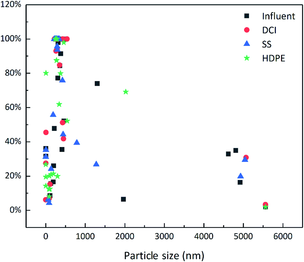Fig. 2 Frequency distribution of particle size in the influent and effluents.

3.2 Characteristics of the tubing inner walls

To understand the corrosion characteristics of the tubing inner wall during operation, two small pieces were taken from each AR before the research, specifically on the 14^th and 25^th days of operation, and the tubing inner walls were scanned by SEM and EDS to analyse the micromorphology and elemental composition of the tubing inner walls.

3.2.1 Micromorphology. Representative SEM images of the tubing inner walls during the different running stages are shown in Fig. 3, where it can be seen that the different tubing materials showed significant differences during operation, and even various different microstructural features could be seen in the same tubing samples.

As shown in Fig. 3, the microstructure of the DCI pipe inner wall was loose and porous in the form of fine sand before running (Fig. 3(a)); then, relatively dense small grains appeared on the 14^th day (Fig. 3(b)), and these became more prominent on the 25^th day (Fig. 3(c)). Bonds et al. reported that the cement-mortar lining of DCI has cracks that can close and thereby the lining becomes tight after a period of exposure to water, but also the cement will eventually undergo autogenous healing, a phenomenon long recognised by the concrete industry and which occurs due to the formation of calcium carbonate and the continuing hydration of cement grains in the lining.⁴⁴

Fig. 3 SEM image of the pipeline inner wall in the three different stages.

The SS pipe inner wall had a loose porous texture before running (Fig. 3(d)); then, obvious corrosion scales on the inner wall structure could be seen on the 14^th day (Fig. 3(e)), and later the corrosion tubercles became smaller, and the inner walls were denser on the 25^th day (Fig. 3(f)). These SEM images of SS are similar with the previous report.^75,76 However, the corrosion of the SS pipe may not be that easy, as Zhang et al. reported that some loose floccus seen on the surface of their sample could represent the metabolites of bacteria.⁴⁰

Before running (Fig. 3(g)), and on the 14^th day (Fig. 3(h)), the HDPE pipe inner walls were smooth, with obvious point-like small holes seen before running; the perforations therein increased, and the damage to the inner wall was clealrly intensified on the 14^th day, and then inner walls had become rough and compact by the 25^th day (Fig. 3(i) and (j)). Leban et al. reported that the corrosion products were deposited especially around the perforation, with the shape of the perforations found on the pipe being of irregular shape with sharp angles.⁷⁵ These SEM images of HDPE are similar with the fouled membranes deposits and bacterial cells in the reports of Ayache et al.⁷⁷ and Rożej et al.⁶⁸, which imply that it is likely to be a change caused by biofilm formation or particle attachment.

3.2.2 Elemental composition. The atomic percentage of the material composition in different stages of the different tubings inner wall, as measured by EDS, are listed in Table 1. Each tubing segment was measured multiple times at observed significant changes, and representative data were selected here for comparison with the SEM images. The elemental composition of the tubing material on the inner walls were determined by the physico-chemical parameters of the tubing inner wall material and the bulk water. It can be seen from Table 1 that the inner wall elemental composition of the same material was similar at each stage, and here, the corroded or perforated parts were more significant for this study than the intact parts, and it was found that in the different pipe sections, the composition of the inner wall material element differed significantly.

Table 1 Composition of material elements on the inner wall of the three types of pipes (at%)^a

Sample	Site	C (%)	O (%)	Na (%)	Mg (%)	Al (%)	Si (%)	S (%)	K (%)	Ca (%)	Fe (%)	Ti (%)	Ni (%)	Mn (%)	F (%)	Cr (%)	Cl (%)
a (1) DCI (0) indicates the DCI pipe before operation, DCI (14) indicates the 14^th day of the DCI pipe AR running, DCI (25) indicates the 25^th day of the DCI pipe AR running, other pipe representation methods are similar. (2) “—” means not detected; corrosion – corrosion site, intact – intact site, perforation – perforation.
DCI(0)		3.80	45.51	0.94	1.89	1.56	4.73	0.35	2.19	36	3.04	—	—	—	—	—	—
DCI(14)	Corrosion	4.48	49.11	—	0.49	0.59	1.28	0.29	—	42.75	1.01	—	—	—	—	—	—
DCI(14)	Intact	9.08	43.40	—	0.56	0.60	12.33	—	—	30.56	0.57	2.90	—	—	—	—	—
DCI(25)	Corrosion	5.77	45.42	—	1.47	1.87	5.61	0.23	0.75	36.03	2.86	0	—	—	—	—	—
DCI(25)	Intact	4.10	44.18	—	0.52	0.56	1.89	—	—	47.12	1.63	—	—	—	—	—	—
SS(0)		—	2.62	—	—	—	0.42	—	—	—	71.11	—	8.62	—	—	17.22	—
SS(14)	Corrosion	—	8.62	—	—	—	0.70	—	—	—	66.61	—	6.89	1.13	—	16.05	—
SS(14)	Intact	—	5.11	—	—	—	—	—	—	—	66.58	—	8.78	—	—	19.53	—
SS(25)	Corrosion	—	11.62	—	—	—	0.67	—	—	—	68.16	—	5.35	—	—	14.19	—
SS(25)	Intact	—	3.67	—	—	—	0.62	—	—	—	70.15	—	8.54	—	—	17.02	—
HDPE(0)	Perforation	77.24	13.11	1.64	—	0.36	0.65	—	1.30	2.58	1.10	—	—	—	—	—	2.02
HDPE(0)	Intact	66.88	20.02	1.55	—	1.41	1.77	0.16	0.96	4.51	2.03	—	—	—	—	—	0.71
HDPE(14)	Perforation	52.75	17.67	—	—	—	23.39	1.94	—	1.23	—	1.59	—	—	—	—	1.44
HDPE(14)	Intact	70.53	15.94	—	—	020	6.05	—	—	3.83	1.65	1.51	—	—	—	—	0.30
HDPE(25)	Perforation	72.47	16.77	—	—	0.40	5.93	—	0.26	1.22	0.90	1.70	—	—	—	—	0.36
HDPE(25)	Intact	49.18	24.42	—	—	0.24	14.58	—	—	0.88	0.93	2.79	—	—	6.38	—	0.61

---

In the composition of the DCI pipe inner wall, O and Ca were the main constituent elements, followed by Si, C, Fe, Mg and Al, which were related to the main components of the lining material (calcium hydroxide and calcium silicate hydrate). It can be seen from Table 1 that the Si content increases with the running time, and Bonds et al. reported that this is caused by the soft dissolution of the cement mortar lining due to the prolonged soaking time.⁴⁴ Moreover, Slaats et al. reported that, when the pH and the calcium content increase, calcium carbonate can precipitate on the pipe walls.⁴³ In the SS pipe inner wall, the elemental composition was such that Fe and Cr were the main components of the SS pipe, and the amounts of Ni, O and Si were relatively small; with only a small amount of Mn detected in the corrosion site on the 14^th day, while O was increased following operation, and this was more significant in the corroded area. HDPE pipe is an organic tubing material, and consequently, the content of C and O was higher, followed by Si, Ca, Cl, Fe and Al in descending order. Among the three tubing materials, the other components of different tubing materials were caused by the tubing itself. From Table 1, it can be found that the sum of the atomic percentage contents of Fe and O was significantly different. The DCI, SS and HDPE pipes contained, respectively, 43.97% to 50.12%, 71.69% to 79.78%, and 14.21% to 25.35%.

3.3 Microbial diversity analysis

Microbiological influenced corrosion (MIC) is a corrosive effect on a pipeline caused by biogenic activity in the pipeline in the presence of microorganisms and their interactions with the environment inside the pipe. Bacteria are one of the most important parameters related to the water quality of a DWDS. Bacteria attach to the tubing inner walls to form a biofilm, which is closely related to the water quality changes in the DWDS.^45,59,78

3.3.1 Microbial diversity and abundance analysis. Uparse software (Uparse v7.0.1001) was used to cluster the Effective Tags of all samples. By default, the sequence was clustered into Operational Taxonomic Units (OTUs) with 97% identity, and the representative sequence of OTUs was selected. According to the principle underpinning its algorithm, the sequence with the highest frequency in OTUs was selected as the representative sequence of OTUs. Specimen annotation of the OTUs representative sequences, species annotation analysis using the Mothur method and SILVA's SSU rRNA database (set threshold of 0.8 to 1), obtaining taxonomic information, and statistically calculating the community composition of each sample at each classification level (kingdom, phylum, class, order, family, genus, species) were undertaken. Fast multi-sequence alignment was performed using MUSCLE (Version 3.8.31) software to obtain a systematic relationship between all the OTUs and the representative sequences. Finally, the data from each sample were homogenised with a standard based on the least amount of data in the sample. Subsequent alpha diversity and beta diversity analyses were based on the data after homogenisation.

Qiime software (Version 1.7.0) was used to calculate the Observed-species, Chao1, Shannon, Simpson, ACE, Goods-coverage and PD_whole_tree indices (Table 2); then Origin software (Version Pro 9.0) was used to draw the rarefaction curve (Fig. S3†).

Table 2 16S rRNA gene library diversity results of the BIPES sequencing analysis

Sample name	Good-coverage	Observed species	Shannon	Simpson	Chao1	ACE	PD-whole-tree
Influent	0.99	2134	6.796	0.938	2475.711	2539.229	133.343
DCI	0.994	1874	6.448	0.947	1964.721	2065.003	114.276
SS	0.991	1889	6.433	0.945	2195.92	2273.004	118.692
HDPE	0.991	2154	7.22	0.975	2466.037	2520.359	129.354

---

The rarefaction curve can be used to assess whether, or not, the amount of sequencing can cover all populations, while at the same time it indirectly reflects the number of species in a sample. In Fig. S3,† the rarefaction curves of the four samples tend to be shallow in slope, indicating that the amount of sequencing data is progressively more reasonable, and the sequencing depth is appropriate, and can thus be used for subsequent analysis. Meanwhile the abundance of species in the four samples was ranked as HDPE > influent > DCI > SS.

Good-coverage characterises the coverage of each sample database, and the larger the sequencing depth index, the smaller the probability of not being detected in the sample sequence. Here, observed species characterises the number of OTUs in the sample. The Shannon index reflects the index of microbial diversity in the sample, whereby the larger its value, the higher the diversity of the sample community. The Simpson index is used to estimate the microbial diversity, and the larger the Simpson value, the more uniform the sample, indicating that the community structure diversity is higher. Chao1 is commonly used in ecology to estimate the total number of species, with higher values indicating more biomass. ACE is a microbial richness index, which is used to estimate the number of OTUs in a community; further, it is proposed by Chao and is one of the indicators most commonly used when assessing the total number of species in an ecosystem, which is different from that produced when using the Chao1 algorithm. PD-whole-tree is an index that reflects the comprehensive diversity of the lineage.

From the analysis of the data in Table 2, the good-coverage value of sequencing was close to 1, indicating that the coverage of bacteria in the sample sequencing was very high, and the sequencing selection depth was appropriate, and thus met the analytical need for bacterial diversity in the sample. Shannon and Simpson are bacterial community diversity indices, and the diversity of bacterial communities was highest in the HDPE tubing, which is likely to be related to more organic matter having been released into the water by HDPE tubes. Chao1 and ACE are bacterial community abundance indices, whereby the higher their values, the higher the diversity or abundance. Here, the abundance of bacterial communities was ranked thus: influent > HDPE > SS > DCI. Microbial community analysis by Zhang et al. also showed that a biofilm from PE pipe had a much higher diversity than that from DCI and SS pipe.⁵⁴

3.3.2 Comparative analysis of the microbial community composition based on the classification level. The types of microbial classification obtained at different classification levels are shown in Table 3. According to the results of the species annotation, the top 10 species with the highest abundance of each sample at each classification level (phylum, class, order, family, genus and species) were selected to generate a column of the relative abundance of the species to assess each sample at different taxonomic levels, and to find relatively high-abundance species and the proportions thereof (Fig. S4†).

Table 3 Classification of microorganisms at the different classification levels^a

Sample name	Phylum	Class	Order	Family	Genus
a The duplicate categories in the sample are combined in the sum.
Influent	34	74	140	240	450
DCI	35	67	132	230	316
SS	32	68	127	222	313
HDPE	32	69	132	237	347
Sum	41	87	171	307	544

---

It can be seen from Table 3 that microorganisms can be classified into 41 phyla, 87 classes, 171 orders, 307 families and 544 genera in the all samples. At each level, the microbial diversity of the three tubing material samples was gradually lower than that of the influent with the refinement of the classification, while the effluent from the HDPE tube had a higher diversity than that of the DCI and SS tubes at different classification levels; this conclusion corresponds to that derived from analysis of the data in Table 2 and is consistent with previous research conclusions.^79,80

As can be seen from the analysis of Fig. S4,† overall, with the refinement of the classification level, the proportion of microorganisms that can be explained by sequencing decreased. It can be found from Fig. S4(a)† that the highest abundance among the four samples at the phylum-level was Proteobacteria (average 72.82%), regardless of the pipe material,^{40,45,81–84} followed by Bacteroidetes (average 8.14%) and Cyanobacteria (average value 7.08%), Actinobacteria (average 3.61%) and Acidobacteria (average value 2.33%), while the remaining percentages were less than 1%, which is consistent with pervious research.^85–87 In addition, a certain amount of 16S rRNA sequences (average of 3.31%) in the four samples could not be assigned to any known bacterial species, but closely matched other unclassified sequences originating from drinking water, possibly indicating the existence of novel bacteria adapted to the DWDS.^{45,83,88–90} During the research, the proportion of Proteobacteria in the effluent (72.82% to 86.87%) was significantly higher than that of the influent (48.45%), while Proteobacteria (86.87%) in the DCI samples was significantly higher than that in the SS (74.28%) and HDPE (81.68%) samples. Compared with the influent (23.33%), the ratios of Bacteroidetes (2.79% to 3.32%) of the three tubing material samples were significantly reduced, indicating that the pipe material significantly affected the different microbial abundances in the bulk water.

3.3.3 Microbiological analysis of pipeline corrosion. The inner surface of the water pipeline gradually forms a stable biofilm under conditions of long-term water-flushing. The pipeline inner wall and the biofilm become a whole, and the interaction makes the whole internal pH, organic matter concentration, inorganic concentration and dissolution of oxygen produce a significant difference from the pipeline inner surface, in which no biofilm exists. The metabolic activities of microorganisms cause different degrees of damage to the pipeline inner wall, which gradually deteriorates over time and causes the water quality of the pipeline to change.³¹

To analyse the effects of microorganisms in the bio-corrosion process in the three tubing materials, based on the microbial dominant community structure in the effluent of the different tubings (Section 3.3.2), the analysis focused on the microorganisms in different pipes, including iron-oxidising bacteria (IOB), iron-reducing bacteria (IRB), sulphur-oxidising bacteria (SOB), sulphur-reducing bacteria (SRB), nitrate-reducing bacteria (NRB), nitrogen-fixing bacteria (NFB) and acid-producing bacteria (APB).^{36,83,91–93} The bacterial communities included in various corrosive microorganisms,⁹⁴ at the genus level, are listed in Table S3.†

The relative abundance of the various corrosive-related bacteria in the influent and different pipeline effluents are shown in Fig. 4. Sphingomonas was dominant in both the influent and effluent of the three tubing material samples (8.9209%, 6.1609%, 7.7781%, and 10.8632%, respectively), followed by Pseudomonas (0.6265%) and Massilia (0.5473%) in the influent, Rhodobacter (1.2033%) and Massilia (0.7555%) in the DCI tube effluent, Aquabacterium (2.8047%) and Massilia (0.6892%) in the SS tube effluent and Acidovorax (4.9221%) and Aquabacterium (1.5092%) in the HDPE tube effluent. It could thus be seen that the different tubing materials affected the different corrosive bacterial communities.^{28,45,82,84,87,95,96}

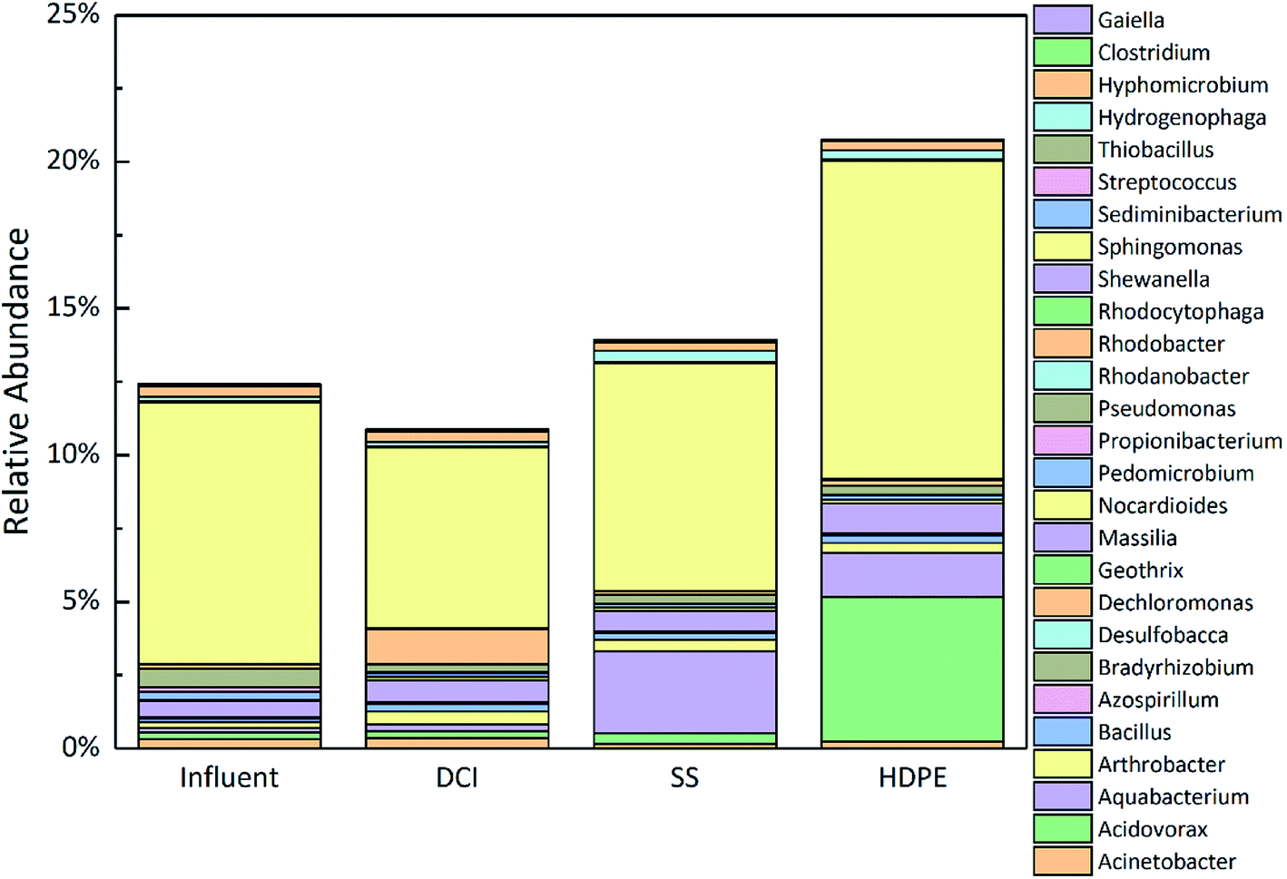Fig. 4 Relative community abundance of corrosion microorganisms at the genus level.

In Fig. 5, the bacterial community was counted according to the different functional types. It was found that NRB was always the most corrosive bacteria in the water from the influent to the effluent. Compared with the pipeline microbial community found in previous research, the relative abundance of the microbial community in this study was relatively low, mainly due to the initial use of new pipelines, and as stable microbial community structures had not yet formed inside the pipeline. Previous researchs has found that Acidovorax (IOB), Aquabacterium (IOB), Sediminibacterium (IOB) and Desulfobacca (SRB) promote corrosion, while Thiobacillus (SOB), Geothrix (IRB), Pseudomonas (IRB) Bacillus (IRB), etc. suppress corrosion.^24,97–99 Therefore, it can be found from the overall microbial community structure that the microbial community that inhibits corrosion in the pipeline gives the main benefit, whereby the deterioration of the water quality of the pipeline is reduced and the corrosion of the inner wall of the pipeline is reduced.

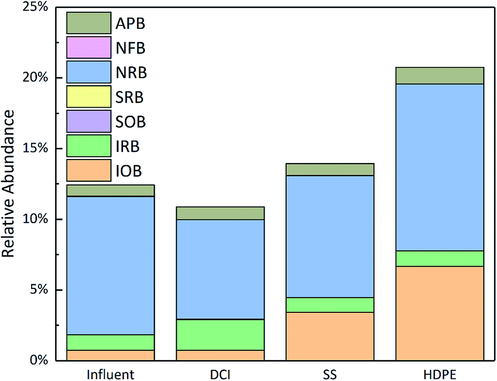Fig. 5 Relative abundance of different corrosive functional bacteria at the genus level.

3.4 Water quality maintenance and pipe material selection suggestion

The water quality change in the SS and the HDPE tubes was consistent, whereby the deterioration was significant in the initial stage, while in the later stage, this gradually stabilised to meet the required water quality standard. Combined with the field water sample collection and analysis in Yantian District, Shenzhen (ESI 2†), it could be determined, only from the sensory properties, that the DCI, SS and the HDPE pipes were stable after the 20^th day, 8^th day and 2^nd day, respectively. It is also recommended that the utility company should flush the DCI and SS pipes on the 8^th day and 2^nd day, respectively.

Based on the influence of the three pipes on the water quality in this test, the SS and HDPE pipes were shown to clearly be more suitable as drinking water pipelines than DCI. Moreover, in the microbial community analysis, the microbial population of HDPE was significantly more than that of SS, which may be the main reason for the preference of SS in the renewal of water supply pipeline in Shenzhen. Schwartz et al. reported reduced bacterial cell densities upon steel compared to plastics (HDPE and PVC), with significant differences in the community composition between the metal and plastics.⁷⁹ Fish et al. reported that standards exist to maintain a high quality of these diverse materials and to minimise their biofilm forming potential (BFP), while BFP variation exists between materials due to differences in their surface characteristics and the likelihood of leaching organics or releasing nutrients when exposed to biological activity, and this has caused much debate in the literature as to which material has the lowest BFP.⁴⁵ Accordingly, the relationship between the pipe material and water quality within DWDS is complex, and based on the results of this study, SS is an ideal drinking water pipeline.

4. Conclusion

Within 25 days, the water quality change in the DCI is the most significant, and the color could reach up to 10 on the 8^th day, and was maintained at 4 in later stages: the turbidity, pH and TOC also increase at the same time, and the decay of residual chlorine and total chlorine was also notable. The conductivity was always maintained at above 0.15 mS cm⁻¹. The DCI inner wall changed from having a loose porous particle shape to a relatively dense, irregular three-dimensional shape, and the constituent elements were mainly O and Ca. The SS inner wall was a uniform structure in the early stage, but there were obvious spherical balls of uneven size seen in the later stage, and its elemental composition comprised mainly C and O. The HDPE inner wall was smooth and had small perforations in the early stage, and these perforations, in the middle and late stages, became enlarged, becoming rough and scale-like in the later stage. The proportion of Proteobacteria in the effluents (72.82% to 86.87%) was significantly increased compared with that in the influent (48.45%), while the Proteobacteria (86.87%) content in the DCI samples was significantly higher than that in the SS (74.28%) and HDPE tubes (81.68%). Moreover, compared with the influent (23.33%), the Bacteroidetes (2.79% to 3.32%) contents of the effluents were significantly reduced, indicating that the pipe material affected different microbial abundances in the water.

Conflicts of interest

There are no conflicts to declare.

Acknowledgements

This work was financially supported by the Major Science and Technology Program for Water Pollution Control and Treatment, National Water Grant (No. 2017ZX07501002-002).

Notes and references

1. G. Liu, Y. Zhang, W. J. Knibbe, C. Feng, W. Liu, G. Medema and W. van der Meer, Water Res., 2017, 116, 135–148.
2. AWW Association, Buried no longer: confronting America's water infrastructure challenge, AWWA, Denver, CO, 2012.
3. J. Q. J. C. Verberk, K. J. O'Halloran, L. A. Hamilton, J. H. G. Vreeburg and J. C. van Dijk, J. Water Supply: Res. Technol.--AQUA, 2007, 56, 345–355.
4. C. R. Proctor and F. Hammes, Curr. Opin. Biotechnol., 2015, 33, 87–94.
5. E. I. Prest, F. Hammes, M. C. van Loosdrecht and J. S. Vrouwenvelder, Front. Microbiol., 2016, 7, 45.
6. A. Nescerecka, T. Juhna and F. Hammes, Water Res., 2018, 135, 11–21.
7. D. v. d. Kooij, J. - Am. Water Works Assoc., 1992, 84, 57–65.
8. M. Li, Z. Liu, Y. Chen and Y. Hai, Water Res., 2016, 106, 593–603.
9. L. Zlatanovic, J. P. van der Hoek and J. H. G. Vreeburg, Water Res., 2017, 123, 761–772.
10. L. S. McNeill and M. Edwards, J. - Am. Water Works Assoc., 2001, 93, 88–100.
11. P. Husband and J. Boxall, Water Res., 2011, 45, 113–124.
12. I. S. Cole and D. Marney, Corros. Sci., 2012, 56, 5–16.
13. A. W. Barker, Anti-Corros. Methods Mater., 1975, 22, 7–9.
14. P. Sarin, V. L. Snoeyink, J. Bebee, K. K. Jim, M. A. Beckett, W. M. Kriven and J. A. Clement, Water Res., 2004, 38, 1259–1269.
15. W. Viessman, M. J. Hammer, E. M. Perez and P. A. Chadik, Water supply and pollution control, Pearson Prentice Hall, New Jersey, 2009.
16. M. Zhang, L. Wang, M. Xu, H. Zhou, S. Wang, Y. Wang, B. Miao and C. Zhang, Sci. Total Environ., 2019, 649, 146–155.
17. F. B. Asghari, J. Jaafari, M. Yousefi, A. A. Mohammadi and R. Dehghanzadeh, Hum. Ecol. Risk Assess., 2018, 24, 1138–1149.
18. P. Smith, Piping Materials Guide, 2005.
19. X. Li, H. Wang, C. Hu, M. Yang, H. Hu and J. Niu, Corros. Sci., 2015, 90, 331–339.
20. Z. Tang, S. Hong, W. Xiao and J. Taylor, Corros. Sci., 2006, 48, 322–342.
21. S. Reiber, S. Poulsom, S. A. Perry, M. Edwards, S. Patel and D. Dodrill, General Framework for Corrosion Control Based on Utility Experience, AWWA, Denver, CO, 1997.
22. S. Price and F. Jefferson, J. N. Engl. Water Works Assoc., 1997, 111, 285–293.
23. F. Yang, B. Shi, J. Gu, D. Wang and M. Yang, Water Res., 2012, 46, 5423–5433.
24. F. Yang, B. Shi, Y. Bai, H. Sun, D. A. Lytle and D. Wang, Water Res., 2014, 59, 46–57.
25. X. Zhang, Z. Mi, Y. Wang, S. Liu, Z. Niu, P. Lu, J. Wang, J. Gu and C. Chen, Front. Environ. Sci. Eng., 2014, 8, 417–426.
26. X. Zhang, Z. Mi, Y. Wang, S. Liu, Z. Niu, P. Lu, J. Wang, J. Gu and C. Chen, Front. Environ. Sci. Eng., 2013, 8, 417–426.
27. I. Douterelo, R. Sharpe and J. Boxall, J. Appl. Microbiol., 2014, 117, 286–301.
28. H. Wang, S. Masters, Y. Hong, J. Stallings, J. O. Falkinham III, M. A. Edwards and A. Pruden, Environ. Sci. Technol., 2012, 46, 11566–11574.
29. M. Heibati, C. A. Stedmon, K. Stenroth, S. Rauch, J. Toljander, M. Save-Soderbergh and K. R. Murphy, Water Res., 2017, 125, 1–10.
30. W. Zhang and F. A. DiGiano, Water Res., 2002, 36, 1469–1482.
31. L. C. Simoes and M. Simoes, RSC Adv., 2013, 3, 2520–2533.
32. S. Tang, D. P. Yue and D. C. Ku, Engineering and costs of dual water supply systems, IWA Publishing, 2007.
33. S. Chu, The reform of the urban water supply in Southern China, Globalization Monitor, 2010.
34. F. Yang, B. Shi, W. Zhang, J. Guo, N. Wu and X. Liu, 2018.
35. I. Gomes, M. Simões and L. C. Simões, Water Res., 2014, 62, 63–87.
36. W. Qiu, W. Li, J. He, H. Zhao, X. Liu and Y. Yuan, J. Environ. Sci., 2018, 74, 177–185.
37. H. Wang, C. Hu, S. Zhang, L. Liu and X. Xing, J. Environ. Sci., 2018, 73, 38–46.
38. H.-C. Su, Y.-S. Liu, C.-G. Pan, J. Chen, L.-Y. He and G.-G. Ying, Sci. Total Environ., 2018, 616, 453–461.
39. J. G. Caporaso, C. L. Lauber, W. A. Walters, D. Berg-Lyons, C. A. Lozupone, P. J. Turnbaugh, N. Fierer and R. Knight, Proc. Natl. Acad. Sci. U. S. A., 2011, 108, 4516–4522.
40. H. Zhang, Y. Tian, M. Kang, C. Chen, Y. Song and H. Li, Chemosphere, 2019, 215, 62–73.
41. A. Deb, S. B. McCammon, J. Snyder and A. Dietrich, Impacts of lining materials on water quality, Water Research Foundation, Denver, 2010, p. 182.
42. D. Ellison, F. Sever, P. Oram, W. Lovins, A. Romer, S. J. Duranceau and G. Bell, Global review of spray-on structural lining technologies, Water Research Foundation, Denver, 2010, pp. 1–184.
43. P. Slaats, G. Mesman, L. Rosenthal and H. Brink, Water Sci. Technol., 2004, 49, 33–39.
44. R. W. Bonds, A. L. Birmingham, Ductile Iron Pipe, 2005.
45. K. E. Fish, A. M. Osborn and J. Boxall, Environ. Sci.: Water Res. Technol., 2016, 2, 614–630.
46. M. N. Sharif, A. Farahat, H. Haider, M. A. Al-Zahrani, M. J. Rodriguez and R. Sadiq, Environ. Monit. Assess., 2017, 189, 307.
47. A. Araya and L. D. Sánchez, J. Water, Sanit. Hyg. Dev., 2018, washdev2018162.
48. Y. Zhao, Y. J. Yang, Y. Shao, J. Neal and T. Zhang, Water Res., 2018, 141, 32–45.
49. M. Vijay, S. Porwal, S. Jain and B. Botre, 2017.
50. E. M. Ringger, A. J. Whelton, T. Odimayomi and M. Salehi, The Summer Undergraduate Research Fellowship (SURF) Symposium, 2018, p. 39.
51. M. N. B. Momba, R. Kfir, S. N. Venter and T. E. Cloete, Water SA, 2000, 26, 59–66.
52. A. Al-Jasser, Water Res., 2007, 41, 387–396.
53. L. A. Rossman, Water Res., 2006, 40, 2493–2502.
54. C. Zhang, C. Li, X. Zheng, J. Zhao, G. He and T. Zhang, Int. J. Environ. Sci. Technol., 2017, 14, 85–94.
55. J. Xu, C. Huang, X. Shi, S. Dong, B. Yuan and T. H. Nguyen, Sci. Total Environ., 2018, 642, 516–525.
56. B. Brazos, J. O'Connor and S. Abcouwer, 1985.
57. N. Hallam, J. West, C. Forster, J. Powell and I. Spencer, Water Res., 2002, 36, 3479–3488.
58. L. Kiéné, W. Lu and Y. Lévi, Water Sci. Technol., 1998, 38, 219–227.
59. K. C. Makris, S. S. Andra and G. Botsaris, Crit. Rev. Environ. Sci. Technol., 2014, 44, 1477–1523.
60. D. Zhong, Y. Yuan, W. Ma, C. Cui and Y. Wu, Desalin. Water Treat., 2012, 49, 165–171.
61. G. Mao, Y. Wang and F. Hammes, Sci. Total Environ., 2018, 613, 1220–1227.
62. L. Zhang, S. Liu and W. Liu, Environ. Sci.: Processes Impacts, 2014, 16, 280–290.
63. J. D. Clogston and A. K. Patri, in Characterization of nanoparticles intended for drug delivery, Springer, 2011, pp. 63–70.
64. M. D. Afonso, G. Hagmeyer and R. Gimbel, Sep. Purif. Technol., 2001, 22, 529–541.
65. C. R. Proctor, M. A. Edwards and A. Pruden, Environ. Sci.: Water Res. Technol., 2015, 1, 882–892.
66. Q. M. Bautista-de los Santos, J. L. Schroeder, M. C. Sevillano-Rivera, R. Sungthong, U. Z. Ijaz, W. T. Sloan and A. J. Pinto, Environ. Sci.: Water Res. Technol., 2016, 2, 631–644.
67. Z. Chen, T. Yu, H. H. Ngo, Y. Lu, G. Li, Q. Wu, K. Li, Y. Bai, S. Liu and H.-Y. Hu, Bioresour. Technol., 2018, 254, 290–299.
68. A. Rożej, A. Cydzik-Kwiatkowska, B. Kowalska and D. Kowalski, World J. Microbiol. Biotechnol., 2015, 31, 37–47.
69. D. Brocca, E. Arvin and H. Mosbæk, Water Res., 2002, 36, 3675–3680.
70. A. Koch, Gas chromatographic methods for detecting the release of organic compounds from polymeric materials in contact with drinking water, Doctoral dissertation, Hygiene-Inst. des Ruhrgebiets, 2004.
71. I. Skjevrak, A. Due, K. O. Gjerstad and H. Herikstad, Water Res., 2003, 37, 1912–1920.
72. S.-H. Chae, D.-H. Kim, D. Y. Choi and C.-H. Bae, Water, 2016, 8, 49.
73. D.-H. Kim, D.-J. Lee, J.-S. Hwang and D.-Y. Choi, J. Korean Soc. Environ. Eng., 2013, 35, 312–320.
74. V. Gauthier, B. Barbeau, R. Millette, J.-C. Block and M. Prevost, Water Sci. Technol.: Water Supply, 2001, 1, 237–245.
75. M. B. Leban and T. Kosec, Eng. Failure Anal., 2017, 79, 940–950.
76. J. Liu, H. Chen, L. Yao, Z. Wei, L. Lou, Y. Shan, S. D. Endalkachew, N. Mallikarjuna, B. Hu and X. Zhou, J. Hazard. Mater., 2016, 317, 27–35.
77. C. Ayache, C. Manes, M. Pidou, J. P. Croué and W. Gernjak, Water Res., 2013, 47, 3291–3299.
78. A. M. Azzam, N. M. Ismail and B. B. Mostafa, Asian Pac. J. Trop. Dis., 2016, 6, 126–132.
79. T. Schwartz, S. Hoffmann and U. Obst, Water Res., 1998, 32, 2787–2797.
80. I. Douterelo, S. Husband and J. B. Boxall, Water Res., 2014, 54, 100–114.
81. I. Douterelo, R. L. Sharpe and J. B. Boxall, Water Res., 2013, 47, 503–516.
82. J. Yu, D. Kim and T. Lee, Water Sci. Technol., 2010, 61, 163.
83. D. Liu, C. Rong, J. Jin, S. Liang and J. Zhang, Environ. Sci.: Water Res. Technol., 2018, 4, 1489–1500.
84. K. Zhang, C. Cao, X. Zhou, F. Zheng, Y. Sun, Z. Cai and J. Fu, Water Res., 2018, 131, 11–21.
85. F. Wang, W. Li, Y. Li, J. Zhang, J. Chen, W. Zhang and X. Wu, Front. Environ. Sci. Eng., 2018, 12, 6.
86. H. Sun, B. Shi, Y. Bai and D. Wang, Sci. Total Environ., 2014, 472, 99–107.
87. H. Wang, S. Masters, M. A. Edwards, J. O. Falkinham III and A. Pruden, Environ. Sci. Technol., 2014, 48, 1426–1435.
88. J. B. Poitelon, M. Joyeux, B. Welte, J. P. Duguet, J. Peplies and M. S. Dubow, Lett. Appl. Microbiol., 2010, 49, 589–595.
89. R. P. Revetta, P. Adin, L. Regina, I. Brandon and J. W. Domingo Santo, Water Res., 2010, 44, 1353–1360.
90. M. Williams, J. Domingo, M. Meckes, C. Kelty and H. Rochon, J. Appl. Microbiol., 2004, 96, 954–964.
91. M. W. Lechevallier, C. D. Lowry, R. G. Lee and D. L. Gibbon, Am. Water Works Assoc., J., 1993, 85, 111–123.
92. J. Jin, G. Wu and Y. Guan, Water Res., 2015, 71, 207–218.
93. F. Teng, Y. T. Guan and W. P. Zhu, Corros. Sci., 2008, 50, 2816–2823.
94. B. H. Rasmus, A. Hans-Jørgen, A. Erik and J. R. Claus, Water Res., 2002, 36, 4477–4486.
95. O. M. Zacheus, M. J. Lehtola, L. K. Korhonen and P. J. Martikainen, Water Res., 2001, 35, 1757–1765.
96. K. Pedersen, Water Res., 1990, 24, 239–243.
97. M. Dubiel, C. Hsu, C. Chien, F. Mansfeld and D. Newman, Appl. Environ. Microbiol., 2002, 68, 1440–1445.
98. L. K. Herrera and H. A. Videla, Int. Biodeterior. Biodegrad., 2009, 63, 891–895.
99. H. Wang, C. Hu, X. Hu, M. Yang and J. Qu, Water Res., 2012, 46, 1070–1078.

---

Footnote

† Electronic supplementary information (ESI) available. See DOI: 10.1039/c8ra08645a

---