DOI:
10.1039/C9NR07425B
(Paper)
Nanoscale, 2019,
11, 21834-21846
Static magnetization of immobilized, weakly interacting, superparamagnetic nanoparticles
Received
28th August 2019
, Accepted 30th October 2019
First published on 31st October 2019
Abstract
The magnetization curve and initial susceptibility of immobilized superparamagnetic nanoparticles are studied using statistical–mechanical theory and Monte Carlo computer simulations. The nanoparticles are considered to be distributed randomly within an implicit solid matrix, but with the easy axes distributed according to particular textures: these are aligned parallel or perpendicular to an external magnetic field, or randomly distributed. The magnetic properties are calculated as functions of the magnetic crystallographic anisotropy barrier (measured with respect to the thermal energy by a parameter σ), and the Langevin susceptibility (related to the dipolar coupling constant and the volume fraction). It is shown that the initial susceptibility χ is independent of σ in the random case, an increasing function of σ in the parallel case, and a decreasing function of σ in the perpendicular case. Including particle–particle interactions enhances χ, and especially so in the parallel case. A first-order modified mean-field (MMF1) theory is accurate as compared to the simulation results, except in the parallel case with a large value of σ. These observations can be explained in terms of the range and strength of the (effective) interactions and correlations between particles, and the effects of the orientational degrees of freedom. The full magnetization curves show that a parallel texture enhances the magnetization, while a perpendicular texture suppresses it, with the effects growing with increasing σ. In the random case, while the initial response is independent of σ, the high-field magnetization decreases with increasing σ. These trends can be explained by the energy required to rotate the magnetic moments with respect to the easy axes.
1. Introduction
Since the 1950s, magnetic particles have been actively used in many technological applications, and especially in magnetic recording and data storage. Magnetic elastomers are produced by embedding magnetic nanoparticles in a rubber matrix, while magnetic fluids are comprised of magnetic nanoparticles suspended in an inert carrier liquid. Single-domain, nanometre-scale magnetic particles can be considered as elementary magnetic units. Embedding a large number of such particles into a matrix makes it possible to control the properties of a composite material using an external magnetic field, and it is this control which is exploited in modern technologies. So-called magnetic soft matter includes ferrofluids,1 magnetorheological fluids, magnetic elastomers2–5 and ferrogels,6–8 ferronematic liquid crystals,9–11 and various biocompatible magnetic suspensions,12–16 which are applied in targeted drug delivery and magnetic hyperthermia.17–22 In addition to technical and biomedical applications, magnetic nanoparticle ensembles are also useful in colloid technology, because of interesting self-assembly processes.23
The fundamental magnetic properties of single superparamagnetic and ferromagnetic nanoparticles have been studied in detail, including the composition and architecture of the particles, and the effects on the static and dynamic responses to applied magnetic fields.24–29 The effects of interactions between magnetic nanoparticles have been investigated experimentally30–32 and in computer simulations.33–37 The links between the basic magnetic properties – such as the dynamic magnetic susceptibility spectrum – and power dissipation38 have been explored in the context of medical applications, such as hyperthermia treatments.39–41 The effects of the carrier liquid on heat dissipation have also been investigated.42
The effects of magnetic interactions on the bulk properties of magnetic liquids are well understood. In particular, the magnetization curve M(H) and the initial susceptibility χ = (∂M/∂H)H=0 of ferrofluids can be predicted accurately using statistical–mechanical theory,43–45 as tested against experimental measurements46 and computer simulations.47–49 In such systems, whether the particles are superparamagnetic or ferromagnetic is unimportant, as long as the particles are free to rotate.
In this work, the response of interacting superparamagnetic nanoparticles (SNPs) immobilized in a solid matrix to an applied magnetic field is studied using statistical–mechanical theory and computer simulations. Here, the SNPs are dispersed uniformly throughout the matrix, while the orientations of the easy axes are subjected to various types of texturing. The orientation of a nanoparticle's magnetic moment is assumed to display uniaxial anisotropy, meaning that there is only one easy axis of alignment. The magnetization curve and the initial susceptibility are therefore controlled by the energy barrier separating the two degenerate alignments of a nanoparticle's magnetic moment with respect to its easy axis, the interaction energy between dipoles and the field, and the interactions between dipoles on different particles. The latter two effects are strongly influenced by the direction and degree of alignment of the easy axes with respect to the applied magnetic field. Herein, parallel, perpendicular, unidirectional, and isotropic distributions are considered. The reason for these choices is that the easy axes can be aligned in a liquid precursor solution using a strong magnetic field before initiating a chemical reaction or physical process that solidifies the suspending medium. The probing field can then be applied at any angle with respect to the easy-axes. The isotropic distribution is, of course, the default situation without any field applied during synthesis. It will be shown theoretically that interactions and textures have huge effects on the magnetic response, and particularly on the magnitude of χ, which is of course anisotropic in the case of the easy axes being aligned. Interactions can only be treated in an approximate manner, and in this work, the first-order modified mean-field (MMF1) approach will be exploited.43–45 The role of magnetic interactions between particles will nonetheless be shown to be substantial, and the accuracy of this approach will be demonstrated by comparison with Monte Carlo (MC) simulations. This type of system has been studied before. Carrey et al. studied the dynamic response of immobilized SNPs with parallel and isotropic distributions of the easy axes, using Stoner-Wohlfarth models and linear-response theory.50 Elrefai et al. established empirical expressions for the magnetization curves of immobilized non-interacting SNPs by fitting to numerical simulations, and then compared the results to experimental data.51 The novelty of the current work is that the static magnetic properties of immobilized SNPs are expressed in analytical form, and with interactions taken into account according to systematic statistical–mechanical theory.
The rest of the article is organized as follows. The essential features of SNPs, and the particle model adopted in this work, are defined in section 2. The statistical–mechanical framework of the theory is outlined in section 3, and the application to immobilized and orientationally textured systems is detailed in section 4. The MC simulations are described in section 5. The results are presented in section 6, in the form of direct comparisons between theory and simulation for various cases of orientational texture. The conclusions are presented in section 7.
2. Superparamagnetic nanoparticles
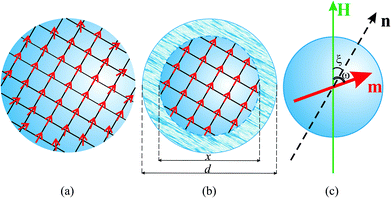
This work concerns the magnetic properties of interacting SNPs with a typical diameter of ∼10 nm, and it is important to define clearly the internal structure of the particles. The particles are considered to be spherical, and smaller than the size of a single magnetic domain in the bulk material. Hence, the particle should be homogeneously magnetized, but the problem is that the magnetization is less than that in the bulk material. Qualitatively, this difference can be explained by the partial frustration of the spin order close to the particle surface, as shown in Fig. 1(a). An additional effect is that, with commonly used iron-oxide materials, incomplete oxidation of the magnetic core leads to a suppression of its magnetic moment. For example, magnetite (Fe3O4) or maghemite (Fe2O3) nanoparticles may actually contain some wustite (FeO).52 As a result of both of these effects, the magnetization of the material becomes dependent on the particle size, and this dependence cannot be calculated easily from first principles. To overcome these problems, a core–shell model is assumed, in which each particle contains an inner, uniformly magnetized spherical core, the magnetization of which is equal to the bulk magnetization of the material; see Fig. 1(b). The core is surrounded by a so-called ‘dead magnetic layer’, which is a non-magnetic shell. Usually, the particles are also covered with an adsorbed layer of surfactant molecules, which provides steric stabilization against irreversible particle coagulation. Thus, the particle is characterized by several dimensions: (i) the diameter of the internal magnetized core x, which determines the particle magnetic moment; (ii) the diameter of the solid part of the particle, which largely determines its mass; and (iii) the hydrodynamic diameter d > x, which includes the magnetized core, the dead layer, and the surfactant layer. d determines both the translational and rotational Brownian mobilities of the particles, which are important for ferrofluids because all translational and rotational degrees of freedom are active. Evidently, in the absence of an external magnetic field, the Brownian motion results in a uniform equilibrium distribution of the orientations of the particle magnetic moments. The core–shell model is very convenient for determining the magnetic interactions between particles, because the interaction between two uniformly magnetized spheres is exactly equivalent to that between two point dipoles, without any multipolar corrections.53
 |
| | Fig. 1 Model of a superparamagnetic nanoparticle. (a) The magnetic ordering of the spins is partially frustrated close to the particle surface, and so the magnetization is less than the magnetization of the bulk material. (b) The core–shell model of the magnetic nanoparticle. The internal magnetic core with diameter x is assumed to be uniformly magnetized without any frustration of the spins. The external particle diameter d > x includes both the non-magnetic surface layer and the adsorbed surfactant layer which prevents particle coagulation. (c) The orientation of the particle is given by the body-fixed, magnetic easy axis vector n. The orientation of the particle magnetic moment m can be different from the easy-axis vector due to superparamagnetic fluctuations. | |
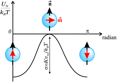
The next issue is the orientation of the magnetic moment m inside the body of a particle. The Brownian translations and rotations of immobilized particles are suppressed, and so the magnetic moment can vary only by superparamagnetic fluctuations (the Néel mechanism). In the simplest case, the crystalline structure of the magnetic material has only one axis of easy magnetization (uni-axis magnetization). Therefore, the orientation of the particle is defined by the direction of the magnetic easy axis, denoted by the vector n; see Fig. 1(c). The magnetic moment of a particle has two degenerate ground-state directions, these being parallel and anti-parallel to the easy axis. The potential energy UN as a function of the angle between m and n is shown schematically in Fig. 2. The energy barrier is proportional to the volume of the magnetic core vm = πx3/6, and the magnetic crystallographic anisotropy constant K, a material property. For common nanosized particles, the barrier (Kvm) may be comparable to the thermal energy, and so thermal fluctuations result in stochastic reorientations of the magnetic moment. The mean value of the particle magnetic moment, measured over a long time, will be equal to zero. This behaviour is known as Néel superparamagnetism, and it is a characteristic of nanosized particles only. Superparamagnetic fluctuations are commonly described as the thermally activated rotations of the magnetic moment inside the particle magnetic core. Importantly, this mechanism means that even if particle positions and orientations (easy axes) are frozen, the magnetic moments are still able to rotate, subject to the potential energy UN, and the interactions with the field and other magnetic moments.
 |
| | Fig. 2 Potential energy UN as a function of the angle between the magnetic moment m and the easy axis n inside a single-domain SNP. The ground states are at angles equal to zero and π radians. The maximum of the energy barrier corresponds to the perpendicular orientation (π/2 radians). The energy is shown in the units of thermal energy kBT. | |
Putting all of this together, the total potential energy of a configuration of N identical SNPs can be written in the form
| |  | (1) |
where the first term contains the single-particle energies, these being the Néel energy (
UN), and the interaction energy between a magnetic moment and an applied field
H (
Um), and the second term includes hard-sphere (
UHS) and dipolar (
Ud) interactions between pairs of particles. The HS potential prevents overlaps of particles with hydrodynamic diameter
d, and the remaining potentials are as follows.
| | UN(i) = −Kvm(![[m with combining circumflex]](https://www.rsc.org/images/entities/b_char_006d_0302.gif) i· i·![[n with combining circumflex]](https://www.rsc.org/images/entities/b_char_006e_0302.gif) i)2 i)2 | (2) |
| | Um(i) = −μ0(mi·H) = −μ0mH(![[m with combining circumflex]](https://www.rsc.org/images/entities/b_char_006d_0302.gif) i·ĥ) i·ĥ) | (3) |
| |  | (4) |
![[m with combining circumflex]](https://www.rsc.org/images/entities/b_char_006d_0302.gif)
and
![[n with combining circumflex]](https://www.rsc.org/images/entities/b_char_006e_0302.gif)
are unit vectors,
μ0 is the vacuum magnetic permeability,
m =
vmM0 is the magnitude of each particle magnetic moment, where
M0 is the magnetization of the bulk material, the applied magnetic field
H has strength
H and orientation
ĥ, and
rij =
rij![[r with combining circumflex]](https://www.rsc.org/images/entities/b_char_0072_0302.gif) ij
ij is the centre–centre separation vector between particles
i and
j. Associated with these interactions are several dimensionless parameters, which measure the corresponding energies with respect to the thermal energy
kBT, where
kB is Boltzmann's constant, and
T is the temperature.
| |  | (5) |
| |  | (6) |
| |  | (7) |
σ is the anisotropy parameter,
λ is the dipolar coupling constant characterizing the particle–particle interactions, and
α is the Langevin parameter characterizing the particle–field interactions.
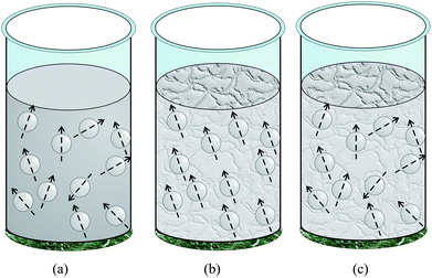
The essential point here is that the magnetic response of immobilized particles is dictated by the internal rotation of the magnetic moments within the particles, rather than by the Brownian rotation of the particles. In sections 3 and 4, the magnetization curve and initial susceptibility will be calculated for systems of particles with various types of orientational distributions of the easy axes (![[n with combining circumflex]](https://www.rsc.org/images/entities/b_char_006e_0302.gif) ). These results will be compared with those for ferrofluids, which will highlight the effects of the textures. The sample geometries and textures studied in this work are illustrated in Fig. 3. Fig. 3(a) represents the case of a ferrofluid, where the particles translate and rotate under the influence of Brownian forces, and the particle–particle and particle–field interactions. Fig. 3(b) shows an immobilized system, where the easy axes are aligned, and the particle positions are random. Fig. 3(c) shows an immobilized system in which the particle positions and easy axes are distributed randomly.
). These results will be compared with those for ferrofluids, which will highlight the effects of the textures. The sample geometries and textures studied in this work are illustrated in Fig. 3. Fig. 3(a) represents the case of a ferrofluid, where the particles translate and rotate under the influence of Brownian forces, and the particle–particle and particle–field interactions. Fig. 3(b) shows an immobilized system, where the easy axes are aligned, and the particle positions are random. Fig. 3(c) shows an immobilized system in which the particle positions and easy axes are distributed randomly.
 |
| | Fig. 3 Sketches of the samples studied: (a) suspension of SNPs undergoing Brownian motion and Néel rotation; (b) immobilized randomly distributed SNPs with perfect alignment of the magnetic easy axes in some direction; (c) immobilized randomly distributed SNPs with no alignment of the magnetic easy axes. In all cases the samples are confined to a highly elongated cylindrical container, with the magnetic field applied along the cylinder axis. The arrows indicate the directions of the easy axes n, and the projections of the magnetic moments m on n can be positive or negative. | |
In all cases, the sample container is taken to be a highly elongated cylinder aligned along the laboratory z axis, and the applied magnetic field H = H(0, 0, 1) is in the same direction. This means that demagnetization effects can be neglected, and the internal magnetic field can be taken to be the same as the external applied field H. The centre-of-mass position of a particle is the radius vector ri = ri![[r with combining circumflex]](https://www.rsc.org/images/entities/b_char_0072_0302.gif) i, where
i, where ![[r with combining circumflex]](https://www.rsc.org/images/entities/b_char_0072_0302.gif) i = (sin
i = (sin![[thin space (1/6-em)]](https://www.rsc.org/images/entities/char_2009.gif) θi
θi![[thin space (1/6-em)]](https://www.rsc.org/images/entities/char_2009.gif) cos
cos![[thin space (1/6-em)]](https://www.rsc.org/images/entities/char_2009.gif) ϕi, sin
ϕi, sin![[thin space (1/6-em)]](https://www.rsc.org/images/entities/char_2009.gif) θi
θi![[thin space (1/6-em)]](https://www.rsc.org/images/entities/char_2009.gif) sin
sin![[thin space (1/6-em)]](https://www.rsc.org/images/entities/char_2009.gif) ϕi, cos
ϕi, cos![[thin space (1/6-em)]](https://www.rsc.org/images/entities/char_2009.gif) θi), θi is the polar angle with respect to the laboratory z axis, and ϕi is the azimuthal angle with respect to the laboratory x axis. The orientation (easy axis) of a particle is the unit vector
θi), θi is the polar angle with respect to the laboratory z axis, and ϕi is the azimuthal angle with respect to the laboratory x axis. The orientation (easy axis) of a particle is the unit vector ![[n with combining circumflex]](https://www.rsc.org/images/entities/b_char_006e_0302.gif) i = (sin
i = (sin![[thin space (1/6-em)]](https://www.rsc.org/images/entities/char_2009.gif) ξi
ξi![[thin space (1/6-em)]](https://www.rsc.org/images/entities/char_2009.gif) cos
cos![[thin space (1/6-em)]](https://www.rsc.org/images/entities/char_2009.gif) ψi, sin
ψi, sin![[thin space (1/6-em)]](https://www.rsc.org/images/entities/char_2009.gif) ξi
ξi![[thin space (1/6-em)]](https://www.rsc.org/images/entities/char_2009.gif) sin
sin![[thin space (1/6-em)]](https://www.rsc.org/images/entities/char_2009.gif) ψi, cos
ψi, cos![[thin space (1/6-em)]](https://www.rsc.org/images/entities/char_2009.gif) ξi), where ξi and ψi are, respectively, the polar and azimuthal angles in the laboratory frame. The magnetic moment on a particle is mi = m
ξi), where ξi and ψi are, respectively, the polar and azimuthal angles in the laboratory frame. The magnetic moment on a particle is mi = m![[m with combining circumflex]](https://www.rsc.org/images/entities/b_char_006d_0302.gif) i, where
i, where ![[m with combining circumflex]](https://www.rsc.org/images/entities/b_char_006d_0302.gif) i = (sin
i = (sin![[thin space (1/6-em)]](https://www.rsc.org/images/entities/char_2009.gif) ωi
ωi![[thin space (1/6-em)]](https://www.rsc.org/images/entities/char_2009.gif) cos
cos![[thin space (1/6-em)]](https://www.rsc.org/images/entities/char_2009.gif) ζi, sin
ζi, sin![[thin space (1/6-em)]](https://www.rsc.org/images/entities/char_2009.gif) ωi
ωi![[thin space (1/6-em)]](https://www.rsc.org/images/entities/char_2009.gif) sin
sin![[thin space (1/6-em)]](https://www.rsc.org/images/entities/char_2009.gif) ζi, cos
ζi, cos![[thin space (1/6-em)]](https://www.rsc.org/images/entities/char_2009.gif) ωi), and ωi and ζi are, respectively, the polar and azimuthal angles in the body-fixed frame of the particle. These vectors are shown in Fig. 1(c). Now the problem is to study the magnetic properties of a system of N particles in a container with volume V at temperature T. The particle concentration ρ = N/V can be expressed in the dimensionless form ρd3, or converted into the hard-sphere volume fraction φ = πρd3/6.
ωi), and ωi and ζi are, respectively, the polar and azimuthal angles in the body-fixed frame of the particle. These vectors are shown in Fig. 1(c). Now the problem is to study the magnetic properties of a system of N particles in a container with volume V at temperature T. The particle concentration ρ = N/V can be expressed in the dimensionless form ρd3, or converted into the hard-sphere volume fraction φ = πρd3/6.
3. Theory
3.1. First-order modified mean-field theory
The magnetization M of the sample is equal to the projection of a randomly chosen magnetic moment (on particle number 1, for example) onto the magnetic field direction (laboratory z axis), weighted by the one-particle distribution function W(1), averaged over all possible orientations, and multiplied by the particle concentration:| |  | (8) |
The integration over the unit vector ![[m with combining circumflex]](https://www.rsc.org/images/entities/b_char_006d_0302.gif) i is defined as
i is defined as
| |  | (9) |
so that

. A similar definition applies to
![[n with combining circumflex]](https://www.rsc.org/images/entities/b_char_006e_0302.gif) i
i,
ξi, and
ψi. The integration over the particle position
ri is defined as
| |  | (10) |
where the domain of integration is a cylinder with volume
V, the radius
R is infinitely larger than the particle diameter in the thermodynamic limit, and

. The saturation magnetization of the system is equal to
M∞ =
ρm. The one-particle distribution function
W(1) is given by the Boltzmann distribution for the
N-particle system averaged over all degrees of freedom except for those of particle 1.
| |  | (11) |
Q is the partition function, given by the integral of the Boltzmann factor exp(−U/kBT) over the degrees of freedom for all N particles. Differentiating eqn (11) with respect to ![[m with combining circumflex]](https://www.rsc.org/images/entities/b_char_006d_0302.gif) 1 gives
1 gives
| |  | (12) |
where
g2(1, 2) is the pair correlation function determining the mutual probability density for two particles (1 and 2) to be found with a particular set of positions and orientations.
| |  | (13) |
It is only the last term in eqn (12) that describes the interparticle correlations. In the limit of low concentration ρ → 0, the system becomes an ideal paramagnetic gas of non-interacting particles. Omitting the correlation term, the ideal one-particle probability density W0(1) is then the solution of
| |  | (14) |
which gives
| |  | (15) |
where
Z0 is the normalization constant.
The next step is to identify the effects of interparticle correlations, represented by the second term in eqn (12). It contains factors of concentration ρ and Ud/kBT ∼ λ, in addition to the dependence of g2(1, 2) on those variables. The following development is limited to the regime of low concentration (ρd3, φ ≪ 1), and weak-to-moderate interactions (λ ∼ 1). The leading-order correction to eqn (12) is of order φλ, and can be separated out by neglecting the concentration dependence of the pair correlation function, and writing it as a product of two one-particle distribution functions:
| | g2(1, 2) = W(1)W0(2)Θ(1, 2) + ![[scr O, script letter O]](https://www.rsc.org/images/entities/char_e52e.gif) (φλ). (φλ). | (16) |
Θ(1, 2) = exp[−UHS(1, 2)/kBT] is the Heaviside step-function, describing the impenetrability of two particles. Combining eqn (12) and (16) gives
| |  | (17) |
where
Ueff(1) represents an additional effective energy term arising from interactions between particle 1 and the other
N − 1 particles.
| |  | (18) |
The solution of eqn (17) is then the one-particle distribution function
| |  | (19) |
Comparing this result with the corresponding equation for the ideal paramagnetic system (15) makes the meaning of −Ueff(1)kBT absolutely clear: it represents the average interaction energy between particle 1 and the effective magnetic field produced by the N − 1 other particles in the system. As a result, this theoretical approach is called the first-order modified mean-field (MMF1) theory.43–45
3.2. Evaluation of Ueff in the case of a highly elongated cylindrical sample
The integration in Ueff (18) can be separated into an average over all possible orientations of the magnetic moment of particle 2, and an integration over all possible positions of particle 2.| | 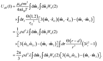 | (20) |
Here the subscript z indicates the z components of the corresponding vectors. The last expression can be written in the succinct form
| | Ueff(1) = (![[m with combining circumflex]](https://www.rsc.org/images/entities/b_char_006d_0302.gif) 1·G) 1·G) | (21) |
where the components of the vector
G=(
Gx,
Gy,
Gz) are defined by
| |  | (22a) |
| |  | (22b) |
| |  | (22c) |
Here χL is the Langevin initial susceptibility
| |  | (23) |
for a system of non-interacting particles. Hence, the interaction correction term is linear in
χL ∼
φλ, which is the essence of the MMF1 theory. The range of validity of the MMF1 approach is
χL ≤ 3.
46,48 An important feature of the MMF1 approach is that
Gz is the component directed along the external magnetic field direction, and is defined similarly to the magnetization
(8). More precisely,
Gz is proportional to the relative magnetization of an ideal system of non-interacting particles, which is determined by the ideal probability density
W0.
3.3. Soft magnetic nanoparticles (σ → 0)
In this limit, the magnetic cores of the SNPs are very small, so that Kvm ≪ kBT. For example, for 5 nm magnetite nanoparticles at room temperature, with a typical value of the magnetic anisotropy constant K ≃ 10 kJ m−3, the dimensionless anisotropy parameter is σ ≃ 0.2. Hence, the intraparticle energy barrier is very low, and the magnetic moment may rotate with respect to the easy axis. Therefore, the orientations of the easy axes are unimportant, and they can be integrated out trivially. In this case, G = (0, 0, χLL(α)) where| |  | (24) |
is the Langevin function. The one-particle distribution function (19) is then| |  | (25) |
where αeff = α + χLL(α) is an effective Langevin parameter, including the interactions between particles. The magnetization and the initial magnetic susceptibility are then given by| |  | (26b) |
These expressions are valid for infinitely soft magnetic nanoparticles irrespective of whether they are suspended in a liquid and may translate or rotate freely, or they are immobilized in some rigid matrix. The only requirement is that the spatial distribution of particles inside the sample is uniform, i.e., no extensive self-assembly induced by magnetic or other colloidal forces takes place. The expressions in eqn (26) are coincident with the MMF1 predictions developed earlier for fluids of spherical particles with central, fixed, point dipoles.44 This equivalence is discussed further in section 4.
3.4. Ferrofluids
The most significant example of a functional material containing magnetic nanoparticles is a ferrofluid.1 The particles are suspended in a carrier liquid [Fig. 3(a)], and undergo both Brownian motion and Néel rotation. Thus, all of the degrees of freedom (![[m with combining circumflex]](https://www.rsc.org/images/entities/b_char_006d_0302.gif) i,
i, ![[n with combining circumflex]](https://www.rsc.org/images/entities/b_char_006e_0302.gif) i, and ri) are active. The vector G depends on W0(2) given by eqn (15), with the normalization constant
i, and ri) are active. The vector G depends on W0(2) given by eqn (15), with the normalization constant| |  | (27) |
where the function| |  | (28) |
was first introduced by Raikher and Shliomis.54 The important point is that Z0(α, σ) is a product of two functions, one of α and one of σ. This means that ![[m with combining circumflex]](https://www.rsc.org/images/entities/b_char_006d_0302.gif) i and
i and ![[n with combining circumflex]](https://www.rsc.org/images/entities/b_char_006e_0302.gif) i are decoupled from one another in ferrofluids. Since the system possesses cylindrical symmetry about the laboratory z axis, the components Gx and Gy are equal to zero. The z component is found to be
i are decoupled from one another in ferrofluids. Since the system possesses cylindrical symmetry about the laboratory z axis, the components Gx and Gy are equal to zero. The z component is found to be| | 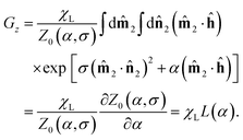 | (29) |
This is precisely the same as the result obtained for soft magnetic nanoparticles in section 3. Therefore, eqn (26) holds true for ferrofluids, and the static (equilibrium) magnetization of a ferrofluid is influenced only by ![[m with combining circumflex]](https://www.rsc.org/images/entities/b_char_006d_0302.gif) i. It means that the easy axes of the particles, at equilibrium, adopt a favourable orientational distribution for a given applied external field due to Brownian rotation. As a result, the static magnetic properties of a fluid suspension of SNPs are independent of the height of the Néel energy barrier σ.
i. It means that the easy axes of the particles, at equilibrium, adopt a favourable orientational distribution for a given applied external field due to Brownian rotation. As a result, the static magnetic properties of a fluid suspension of SNPs are independent of the height of the Néel energy barrier σ.
The MMF1 prediction (26) and its second-order correction (MMF2) were obtained almost twenty years ago for dipolar fluids that correspond to magnetically hard ferroparticles, with σ ≫ 1.43 Nonetheless, the MMF approach describes the static magnetic properties of real ferrofluids containing SNPs rather accurately,46 because the Brownian rotation means that the easy axes cannot influence the equilibrium distribution of the magnetic moments. The same MMF1 results also apply to soft magnetic particles (σ → 0) because the Néel rotation of the magnetic moments is unhindered. The static magnetic properties of dipolar fluids have been well studied by means of computer simulations (both MC and molecular dynamics), and the high accuracy of the MMF1 expressions has been demonstrated over the range χL ≤ 3.46,48 Higher-order corrections for treating concentrated ferrofluids at low temperatures have also been derived.47,49
4. Immobilized nanoparticles
In this section, the static magnetic properties of immobilized SNPs will be calculated, assuming a uniform distribution of particles throughout an elongated cylindrical sample. This case differs strongly from those considered in sections 3.3 and 3.4 because the Brownian motion is suppressed, and the Néel rotation may be hindered. Instead, the easy axes are distributed in fixed configurations, according to several different textures: parallel texture (section 4.1), perpendicular texture (section 4.2), unidirectional texture (section 4.3), and a random distribution (section 4.4).
4.1. Parallel texture
Parallel texturing means that all of the easy axes are aligned parallel to the laboratory z axis, i.e., ![[n with combining circumflex]](https://www.rsc.org/images/entities/b_char_006e_0302.gif) i = (0, 0, 1). It corresponds to the illustration in Fig. 3(b), but with all of the easy axes aligned along the cylinder axis. This means that (
i = (0, 0, 1). It corresponds to the illustration in Fig. 3(b), but with all of the easy axes aligned along the cylinder axis. This means that (![[m with combining circumflex]](https://www.rsc.org/images/entities/b_char_006d_0302.gif) i·
i·![[n with combining circumflex]](https://www.rsc.org/images/entities/b_char_006e_0302.gif) i) = (
i) = (![[m with combining circumflex]](https://www.rsc.org/images/entities/b_char_006d_0302.gif) i·ĥ) = cos
i·ĥ) = cos![[thin space (1/6-em)]](https://www.rsc.org/images/entities/char_2009.gif) ωi. The ideal-gas one-particle distribution function is
ωi. The ideal-gas one-particle distribution function is| |  | (30) |
where| |  | (31) |
Note that R1(α, 0) = sinh(α)/α. By symmetry, Gx = Gy = 0, and the z component is
| |  | (32) |
where
| |  | (33) |
| |  | (34) |
Note that R2(α, 0) = L(α)sinh(α)/α. Substituting these expressions into eqn (21) and (19), gives for the magnetization
| |  | (35) |
where
| |  | (36) |
is the effective Langevin parameter including the interactions between particles. The initial susceptibility is given by
| |  | (37) |
where
| |  | (38) |
Note that R1(0, σ) = R(σ), and the function A‖(σ) coincides with the corresponding value introduced by Raikher and Shliomis.54 For magnetically soft particles, A‖(0) = 1, and then eqn (35) and (37) coincide with (26). The limit of magnetically hard particles (σ → ∞) gives A‖ → 3 and the largest value of the initial magnetic susceptibility, χ‖ → 3χL(1 + χL). This limit is worth mentioning because it corresponds to the case of Ising particles, the magnetic moments of which are quantized in only two states: ![[m with combining circumflex]](https://www.rsc.org/images/entities/b_char_006d_0302.gif) i = ±1. The magnetization (35) in this limit becomes
i = ±1. The magnetization (35) in this limit becomes
| | M‖ → M∞![[thin space (1/6-em)]](https://www.rsc.org/images/entities/char_2009.gif) tanh(α + χL tanh(α + χL![[thin space (1/6-em)]](https://www.rsc.org/images/entities/char_2009.gif) tanh tanh![[thin space (1/6-em)]](https://www.rsc.org/images/entities/char_2009.gif) α) α) | (39) |
which is similar to
eqn (26a) but with the Langevin function
L(
α) replaced by the faster growing function tanh
![[thin space (1/6-em)]](https://www.rsc.org/images/entities/char_2009.gif) α
α. The typical behaviour of the magnetization
(35) is illustrated in
Fig. 4(a) with
σ = 0, 3, and 10, and a rather large value of the Langevin susceptibility
χL = 2 chosen to magnify the effect. Interactions lead to higher magnetization in comparison with non-interacting particles, and the magnetization also increases with increasing anisotropy parameter
σ.
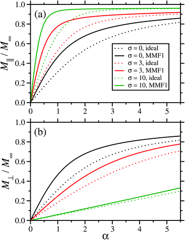 |
| | Fig. 4 Static magnetization curves for immobilized particles with χL = 2, and with parallel (a) and perpendicular (b) textures of the magnetic easy axes. The results are plotted as the reduced magnetization M/M∞ as a function of the dimensionless magnetic field strength (Langevin parameter) α. The dashed lines are for non-interacting (NI) particles, and the solid lines are the theoretical predictions for interacting particles according to eqn (35) (a) and eqn (44) (b). The relative anisotropy energies are σ = 0 (black), 3 (red), and 10 (green). | |
4.2. Perpendicular texture
Perpendicular texturing is when all of the easy axes are aligned parallel to the laboratory x axis, and hence perpendicular to the applied field, i.e., ![[n with combining circumflex]](https://www.rsc.org/images/entities/b_char_006e_0302.gif) i = (1, 0, 0). This means that (
i = (1, 0, 0). This means that (![[m with combining circumflex]](https://www.rsc.org/images/entities/b_char_006d_0302.gif) i·
i·![[n with combining circumflex]](https://www.rsc.org/images/entities/b_char_006e_0302.gif) i) = sin
i) = sin![[thin space (1/6-em)]](https://www.rsc.org/images/entities/char_2009.gif) ωi
ωi![[thin space (1/6-em)]](https://www.rsc.org/images/entities/char_2009.gif) cos
cos![[thin space (1/6-em)]](https://www.rsc.org/images/entities/char_2009.gif) ζi, and (
ζi, and (![[m with combining circumflex]](https://www.rsc.org/images/entities/b_char_006d_0302.gif) i·ĥ) = cos
i·ĥ) = cos![[thin space (1/6-em)]](https://www.rsc.org/images/entities/char_2009.gif) ωi. The ideal-gas one-particle distribution function is
ωi. The ideal-gas one-particle distribution function is| |  | (40) |
where| |  | (41) |
Note that R3(α, 0) = R1(α, 0) = sinh(α)/α. By symmetry, Gx = Gy = 0, and the z component is
| |  | (42) |
where
| |  | (43) |
Note that R4(α, 0) = R2(α, 0) = L(α)sinh(α)/α. Here I0(z) and I1(z) are the modified Bessel functions of zero and first orders, respectively. Following the same development as in the parallel-texture case, the magnetization in the perpendicular case is
| |  | (44) |
where
| |  | (45) |
is the effective Langevin parameter including the interactions between particles. The initial susceptibility is
| |  | (46) |
where
| |  | (47) |
For magnetically soft particles, A⊥(0) = 1, and eqn (44) and (46) coincide with (26). For magnetically hard particles, A⊥(∞) = 0, and χ⊥ = 0.
Similar to the parallel-texture case, the interparticle interactions lead to an increase in the magnetization, as shown in Fig. 4(b). But the growth of the anisotropy parameter results in the opposite effect, because for higher barriers, a stronger magnetic field is required to rotate the magnetic moment away from the easy axis. Hence, the magnetization is a decreasing function of σ in this case.
4.3. Unidirectional texture
In the general case of perfect alignment [Fig. 3(b)], the easy axes are oriented at an angle ξ with respect to the magnetic field; see Fig. 1(c). In this case, ![[n with combining circumflex]](https://www.rsc.org/images/entities/b_char_006e_0302.gif) i = (sin
i = (sin![[thin space (1/6-em)]](https://www.rsc.org/images/entities/char_2009.gif) ξ
ξ![[thin space (1/6-em)]](https://www.rsc.org/images/entities/char_2009.gif) cos
cos![[thin space (1/6-em)]](https://www.rsc.org/images/entities/char_2009.gif) ψ, sin
ψ, sin![[thin space (1/6-em)]](https://www.rsc.org/images/entities/char_2009.gif) ξ
ξ![[thin space (1/6-em)]](https://www.rsc.org/images/entities/char_2009.gif) sin
sin![[thin space (1/6-em)]](https://www.rsc.org/images/entities/char_2009.gif) ψ, cos
ψ, cos![[thin space (1/6-em)]](https://www.rsc.org/images/entities/char_2009.gif) ξ), so that (
ξ), so that (![[m with combining circumflex]](https://www.rsc.org/images/entities/b_char_006d_0302.gif) i·
i·![[n with combining circumflex]](https://www.rsc.org/images/entities/b_char_006e_0302.gif) i) = sin
i) = sin![[thin space (1/6-em)]](https://www.rsc.org/images/entities/char_2009.gif) ξ
ξ![[thin space (1/6-em)]](https://www.rsc.org/images/entities/char_2009.gif) sin
sin![[thin space (1/6-em)]](https://www.rsc.org/images/entities/char_2009.gif) ωi cos(ζi − ψ) + cos
ωi cos(ζi − ψ) + cos![[thin space (1/6-em)]](https://www.rsc.org/images/entities/char_2009.gif) ξ
ξ![[thin space (1/6-em)]](https://www.rsc.org/images/entities/char_2009.gif) cos
cos![[thin space (1/6-em)]](https://www.rsc.org/images/entities/char_2009.gif) ωi, and (
ωi, and (![[m with combining circumflex]](https://www.rsc.org/images/entities/b_char_006d_0302.gif) i·ĥ) = cos
i·ĥ) = cos![[thin space (1/6-em)]](https://www.rsc.org/images/entities/char_2009.gif) ωi. An important difference from the preceding cases is that the one-particle distribution function becomes dependent on the angles ξ and ψ.
ωi. An important difference from the preceding cases is that the one-particle distribution function becomes dependent on the angles ξ and ψ.| |  | (48) |
Here
| |  | (49) |
with the special cases R5(α, 0, ξ) = R1(α, 0) = sinh(α)/α, R5(α, σ, 0) = R1(α, σ), and R5(α, σ, π/2) = R3(α, σ). The x and y components of G are in general non-zero, and complicated, but they do not affect the magnetization, which is in the z direction. The z component is
| |  | (50) |
where
| |  | (51) |
and R6(α, 0, ξ) = R2(α, 0) = L(α)sinh(α)/α. For the arbitrary angle ξ, the z component of the magnetization is given by
| |  | (52) |
where the effective Langevin parameter is
| |  | (53) |
The initial susceptibility is
| |  | (54) |
where
| |  | (55) |
It is interesting that there is a magic angle  at which the coefficient Aξ(σ, ξ0) = 1 and is hence independent of σ. At this angle, the initial susceptibility of immobilized SNPs is given by the soft magnetic particle/ferrofluid expression in eqn (26b).
4.4. Random distribution of particle easy axes
The final case considered here is the isotropic – or random – distribution of easy axes, depicted in Fig. 3(c). To be precise, the probability density function of −1 ≤ cos![[thin space (1/6-em)]](https://www.rsc.org/images/entities/char_2009.gif) ξ ≤ 1 is uniform. For a particle with its easy axes at an angle ξ1 with respect to the laboratory z axis, the ideal one-particle distribution function is W0(1) (48). Note that this function is dependent on ξ1 in both the exponent of the numerator, and the normalization coefficient R5 in the denominator. So, to calculate the z component of the effective dipole field (21), one has to average the ratio R6/R5 over the angle ξ1, and the magnetization becomes
ξ ≤ 1 is uniform. For a particle with its easy axes at an angle ξ1 with respect to the laboratory z axis, the ideal one-particle distribution function is W0(1) (48). Note that this function is dependent on ξ1 in both the exponent of the numerator, and the normalization coefficient R5 in the denominator. So, to calculate the z component of the effective dipole field (21), one has to average the ratio R6/R5 over the angle ξ1, and the magnetization becomes| |  | (56) |
where the effective Langevin parameter is also an average, over a second angle ξ2:| |  | (57) |
To calculate the initial susceptibility, it is necessary to first linearize the effective Langevin parameter with respect to the bare Langevin parameter. For small values of α,
| |  | (58) |
Therefore, the effective field is independent of the anisotropy parameter σ, and the initial susceptibility is equal to the usual MMF1 expression for soft magnetic particles and ferrofluids:
| |  | (59) |
Typical magnetization curves are shown in Fig. 5 for both interacting and non-interacting particles with χL = 2. It is clear that the initial linear response of the magnetization is independent of the anisotropy parameter σ. But the approach to the saturation magnetization is much slower with a large value of σ, and as in all of the preceding cases, interactions increase the magnetization for a given field strength.
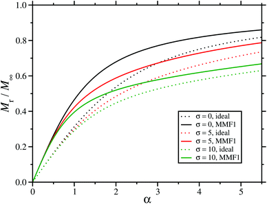 |
| | Fig. 5 Static magnetization curves for immobilized particles with χL = 2, and with random orientations of the magnetic easy axes. The results are plotted as the reduced magnetization M/M∞ as a function of the dimensionless magnetic field strength (Langevin parameter) α. The dashed lines are for non-interacting particles, and the solid lines are the theoretical predictions for interacting particles according to eqn (56). The relative anisotropy energies are σ = 0 (black), 5 (red), and 10 (green). | |
5. Monte Carlo simulations
To test the obtained theoretical predictions, and to determine the range of validity of the MMF1 theory, MC simulations were carried out in the canonical (NVT) ensemble.55 Random configurations of N = 500 dipolar hard spheres were generated in a cubic box of volume V, by sequentially inserting particles at random positions, subject to there being no overlaps. Then, depending on the texture, an easy axis was assigned to each particle. For both parallel and perpendicular textures, the easy axes were unit vectors parallel to the laboratory z axis (the identification of x and z axes being arbitrary in the simulations). For the random texture, the easy axes were randomly generated unit vectors. Periodic boundary conditions were applied, and particle interactions were computed using the Ewald summation with conducting boundary conditions, so as to eliminate all demagnetization effects. Two types of reorientation move were attempted, with equal probability. The first one was a conventional random displacement, with a maximum rotation angle about a random axis tuned to give an acceptance rate of 50%. The second one was a flip move m → −m, which was needed to overcome the anisotropy barrier, particularly with large values of σ. One MC cycle consisted of one attempted move for each of N randomly selected particles. A typical run consisted of 5 × 10⁵ MC cycles after equilibration. Simulations were carried out with dipolar coupling constant λ = 1, and volume fractions φ = 0.02 and 0.05. As a check of the simulation algorithm, and particularly the flip move with large values of σ, some calculations were done for non-interacting systems for comparison with the exact theoretical results. Eight independent configurations were studied for each system and texture, and the results were averaged.
The initial susceptibility in the x direction was computed using the fluctuation formula
| |  | (60) |
where
Mx is a component of the instantaneous magnetization

. Similar equations hold for the
y and
z directions. In the random-texture case,
χr = (
χx +
χy +
χz)/3. With parallel and perpendicular textures,
χ‖ =
χz, and
χ⊥ = (
χx +
χy)/2. The magnetization curves were computed by applying appropriate fields in the
x direction (perpendicular texture) or
z direction (parallel and random textures).
6. Results
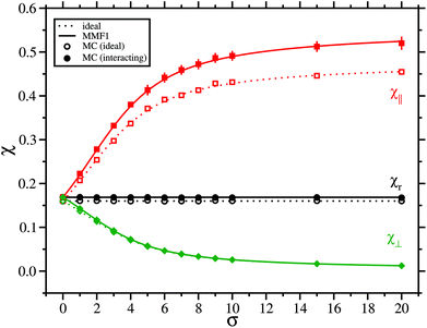
Systems at very low volume fraction φ = 0.02, and with λ = 1, are considered first. These are magnetically very weak, in the sense that the Langevin susceptibility is only χL = 0.16. MC data for the static initial susceptibility, and the corresponding theoretical predictions, are shown in Fig. 6. Results are shown for both interacting and non-interacting systems, and with parallel, perpendicular, and random textures. The first point is that the MC data confirm the qualitative theoretical predictions: the susceptibility for the random distribution is independent of σ for both the interacting and non-interacting systems. The susceptibility for the parallel texture increases with σ, while the susceptibility decreases for the perpendicular texture. Interactions lead to increases in the susceptibility, and here the MMF1 theory is sufficient to give a very accurate description of the magnetic properties. The results for the parallel texture display a surprising effect: even for this weakly interacting system, the difference between the susceptibilities of the non-interacting and interacting particles is unexpectedly large (red squares and red lines), and this difference grows with increasing σ. It means that immobilized SNPs with the easy axes aligned with the field are very sensitive to interparticle magnetic correlations. This can be understood in terms of the long-range nature of the dipole–dipole interaction and the role of orientational averaging; this will be discussed further at the end of this section.
 |
| | Fig. 6 The initial magnetic susceptibility χ as a function of the anisotropy parameter σ for systems with λ = 1 and φ = 0.02, so that χL = 0.16. The solid lines and filled points are for interacting systems, and the dashed lines and unfilled points are for non-interacting systems. Results are shown for random (r, black circles and lines), parallel (‖, red squares and lines), and perpendicular (⊥, green diamonds and lines) textures. | |
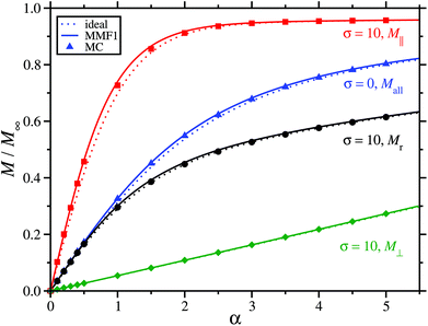
The magnetization curves of dilute systems with various textures are shown in Fig. 7. With σ = 0, the magnetization curves are of course coincident for all textures. With σ = 10, the magnetization for the parallel texture grows rapidly with the applied field, while the magnetization remains low for the perpendicular texture. This is obviously consistent with the initial-susceptibility results presented in Fig. 6. For the random distribution, the initial slope is the same as that for the σ = 0 case, since the initial susceptibility is independent of σ, but the high-field behaviour is different due to the energetic cost of rotating the magnetic moments with respect to the easy axes; this effect was demonstrated already in Fig. 5. In all cases, the effects of interactions are weak, but they are nonetheless described well by the MMF1 theory, eqn (35), (44), and (56). Note that results are shown for σ = 10, but the behaviour of the magnetization curves is typical. As demonstrated in Fig. 4 and 5, the magnetization increases with increasing σ in the parallel case, and decreases in the random and perpendicular cases.
 |
| | Fig. 7 The magnetization M as a function of the Langevin parameter α for systems with λ = 1 and φ = 0.02. The solid lines and filled points are for interacting systems, and the dashed lines are for non-interacting systems. Results are shown for random (r, black circles and lines), parallel (‖, red squares and lines), and perpendicular (⊥, green diamonds and lines) textures with σ = 10, and for a system with σ = 0 (all textures, blue triangles and lines). | |
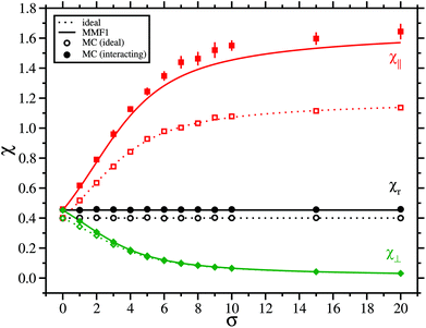
The initial susceptibilities of systems with φ = 0.05 and λ = 1 are shown in Fig. 8. The qualitative behaviour is no different from that of the more-dilute system, but the effects of interactions are more pronounced in this case. For the random and perpendicular textures, the MMF1 theory gives an excellent account of the interactions, with practically no deviation from the MC data. But for the parallel texture, there is a surprising effect: for non-interacting particles, the MC data agree exactly with the theory over the whole range of σ, showing that the flip algorithm is working as intended; but at the same time, the MMF1 susceptibility of interacting particles (37) appears to be valid only for low-to-moderate values of σ. Here, the MC susceptibility increases with σ more rapidly than the prediction of the model (filled red squares and solid red line). Moreover, with high values of σ, the susceptibility of interacting particles is about forty percent larger than that of non-interacting particles, despite the system being only weakly magnetic, with a Langevin susceptibility χL = 0.40. Increasing the concentration further does not change these trends (data not shown): the model (37) agrees well with MC data with low values of σ, but it underestimates the simulated susceptibility with large values of σ.
 |
| | Fig. 8 The initial magnetic susceptibility χ as a function of the anisotropy parameter σ for systems with λ = 1 and φ = 0.05, so that χL = 0.40. The solid lines and filled points are for interacting systems, and the dashed lines and unfilled points are for non-interacting systems. Results are shown for random (r, black circles and lines), parallel (‖, red squares and lines), and perpendicular (⊥, green diamonds and lines) textures. | |
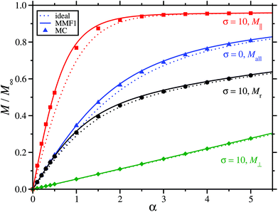
The corresponding magnetization curves for systems with σ = 0 and σ = 10 are shown in Fig. 9. On the whole, the agreement between theory and simulation is good: the effects of texture and the interactions are captured well by the theory. Qualitatively, the trends are the same as those discussed in connection with Fig. 7, but with the increased interactions giving a greater enhancement of the magnetization for a given texture and magnetic-field strength.
 |
| | Fig. 9 The magnetization M as a function of the Langevin parameter α for systems with λ = 1 and φ = 0.05. The solid lines and filled points are for interacting systems, and the dashed lines are for non-interacting systems. Results are shown for random (r, black circles and lines), parallel (‖, red squares and lines), and perpendicular (⊥, green diamonds and lines) all textures with σ = 10, and for a system with σ = 0 (alltextures, blue triangles and lines). | |
The comparison with simulation shows that the MMF1 theory is accurate at least for χL ≤ 0.40. In many biomedical applications, the volume fractions of magnetic material may be an order of magnitude smaller than those considered here. For instance, if φ ∼ 10–3, then with λ = 1, χL ∼ 10–2. The effects of interactions can be assessed using the initial magnetic susceptibility (χ, with interactions) divided by the ideal susceptibility (χideal, without interactions). For the random texture, this ratio is simply
| |  | (61) |
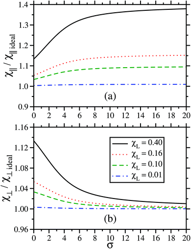
and it is independent of σ. Taking this texture as a guide, enhancements of around 10% are to be expected when χL is about 0.3. Fig. 10 shows the ratios for parallel and perpendicular textures, and with χL = 0.01, 0.10, 0.16, and 0.40. Fig. 10(a) shows that over the range 0 ≤ σ ≤ 20, interactions within the parallel texture enhance the initial magnetic susceptibility by less than 1% with χL = 0.01, 3.3–9.5% with χL = 0.10, 5.3–15% with χL = 0.16, and 13–38% with χL = 0.40. With the perpendicular texture, the enhancements for σ = 0 are the same as with the random and parallel textures, and they decrease with increasing σ. The effects of interactions on χ are obviously mirrored in the initial, linear portion of the magnetization curve (not shown), but the effects on the magnetization decrease with increasing field strength due to the field–particle interactions overcoming the particle–particle interactions.
 |
| | Fig. 10 The initial magnetic susceptibility (χ) divided by the ideal susceptibility (χideal) as a function of the anisotropy parameter σ with parallel (a) and perpendicular (b) textures. Results are shown for systems with χL = 0.40 (black solid line), 0.16 (red dotted line), 0.10 (green dashed line), and 0.01 (blue dot-dashed line). | |
Summing up this section, a comparison of theoretical and simulation results shows that the effects of interactions on the initial static magnetic response of immobilized SNPs are much stronger when the easy axes are aligned parallel with the external field direction, than when they are randomly distributed or perpendicular to the field. While the MMF1 theory (accurate to leading order in the Langevin susceptibility χL) gives excellent predictions in the random and perpendicular cases, it is only accurate in the parallel case when the magnetic crystallographic anisotropy barrier Kvm is not too large compared to the thermal energy kBT (σ ∼ 1). This last condition means that the magnetic moment is not ‘blocked’ inside the body of the particle.
With large energy barriers (σ ≫ 1), the magnetic moments in the parallel texture appear to be strongly correlated, which results in a strong enhancement of the magnetic response, and especially the initial susceptibility. This can be explained in terms of the effect of orientational averaging on the range and strength of the (effective) interactions and correlations between the particles. With low-to-moderate values of σ, the superparamagnetic rotation is not blocked, and the orientational averaging produces an effective interaction between particles that is short ranged (∼−1/rij6). Hence, the resulting correlations are weak. With large values of σ, all of the particle magnetic moments are approximately (anti-)parallel to one another, and hence the dipolar interactions and the resulting correlations are long-ranged (∼1/rij3). Here, the interactions between particles are evaluated on the basis of two-particle correlations (17), and the many-body contributions to the pair correlation function should be included to improve the accuracy of the theory.
Orientational averaging also explains the relatively weak effects of interactions on the initial susceptibility with random and perpendicular textures. In these cases, the effective interactions are short-ranged, due to the azimuthal rotations of the magnetic moments in the perpendicular case, and the isotropic distribution of easy axes in the random case. Hence, the orientational correlations and the enhancement of the initial susceptibility are weak.
7. Conclusions
A theoretical and simulation study of immobilized SNPs has shown the dependence of the static magnetic response on the orientational texture of the easy axes, and the effects of interactions between particles. The particle model included the energy barrier to Néel rotation, and the particle–field and particle–particle interactions. In all cases, the SNPs were distributed randomly in an implicit solid matrix. The theory includes corrections to the non-interacting case at the MMF1 level, i.e., to an accuracy proportional to the Langevin susceptibility χL. Several distributions of the SNP easy axes were considered, all with respect to an external magnetic field: parallel, perpendicular, unidirectional, and random. Connections were made with the relevant limiting cases of soft magnetic particles (σ = 0) and ferrofluids (magnetically hard particles undergoing Brownian translation and rotation). The theoretical predictions were compared with numerical results from MC simulations.
The initial susceptibility χ was found to depend on σ in very different ways, depending on the texture. With a random distribution, χ is independent of σ. With a parallel texture, χ increases with increasing σ, while with a perpendicular texture, χ decreases. In all cases, including interactions between particles leads to an enhancement of χ, but the enhancement is much stronger for the parallel texture than for the random and perpendicular textures. The MMF1 theory is accurate for the random and perpendicular cases with all values of σ, but for the parallel case, it is only reliable with small values of σ. All of these effects can be explained in terms of the effective interactions between the particles, after taking into account orientational averaging of the magnetic moments. When the magnetic moments are blocked and aligned parallel with the external magnetic field, the correlations that control the initial susceptibility are strong and long-ranged. The susceptibility in the random and perpendicular cases remains relatively low because of the possibility of orientational averaging, which renders the correlations short-ranged. Qualitatively, the theory captures all of the main effects of textures and interactions on the initial susceptibility.
The magnetization curves show several interesting features. Although the initial susceptibility of the random texture does not depend on σ, the high-field behaviour does, with the magnetization decreasing with increasing σ. This is due to the increasing energetic cost of rotating the magnetic moments with respect to the easy axes. The magnetization is strongly enhanced by a parallel texture, due to the alignment of the magnetic moments with the easy axes and the field. In contrast, the magnetization is strongly suppressed by a perpendicular texture, as it is restrained by the easy axes. The agreement between the MMF1 theory and MC simulation data is generally good, as the particle–field interaction energy becomes at least as significant as the particle–particle interaction energy.
The basic magnetic properties of immobilized SNPs are becoming increasingly important, due to the development of magnetic gels, elastomers, rubbers, glasses, etc. This work represents a significant step towards a detailed quantitative description of this technologically important class of functional materials.
Conflicts of interest
There are no conflicts of interest to declare.
Acknowledgements
A. O. I. and E. A. E. gratefully acknowledge research funding from the Ministry of Science and Higher Education of the Russian Federation (Contract No. 02.A03.21.006, Project No. 3.1438.2017/4.6).
References
-
R. E. Rosensweig, Ferrohydrodynamics, Dover Publications, Inc., New York, 1998 Search PubMed.
- S. R. Mishra, M. D. Dickey, O. D. Velev and J. B. Tracy, Nanoscale, 2016, 8, 1309–1313 RSC.
- P. Sanchez, T. Gundermann, A. Dobroserdova, S. Kantorovich and S. Odenbach, Soft Matter, 2018, 14, 2170–2183 RSC.
- R. Weeber, M. Hermes, A. Schmidt and C. Holm, J. Phys.: Condens. Matter, 2018, 30, 063002 CrossRef PubMed.
- P. A. Sanchez, E. S. Minina, S. S. Kantorovich and E. Y. Kramarenko, Soft Matter, 2019, 15, 175–189 RSC.
- A. Shankar, A. Safronov, E. Mikhnevich, I. Beketov and G. Kurlyandskaya, Soft Matter, 2017, 13, 3359–3372 RSC.
- F. Blyakhman, N. Buznikov, T. Sklyar, A. Safronov, E. Golubeva, A. Svalov, S. Sokolov, G. Melnikov, I. Orue and G. Kurlyandskaya, Sensors, 2018, 18, 872 CrossRef PubMed.
- G. Kurlyandskaya, S. Shcherbinin, S. Volchkov, S. Bhagat, E. Calle, R. Pérez and M. Vazquez, J. Magn. Magn. Mater., 2018, 459, 154–158 CrossRef CAS.
- T. Tóth-Katona, P. Salamon, N. Éber, N. Tomašovičová, Z. Mitróová and P. Kopčanský, J. Magn. Magn. Mater., 2014, 372, 117–121 CrossRef.
- Y. Raikher and V. Stepanov, J. Mol. Liq., 2018, 267, 367–376 CrossRef CAS.
- Y. Ji, F. Fan, S. Xu, J. Yu and S. Chang, Nanoscale, 2019, 11, 4933–4941 RSC.
- S. Garcia-Jimeno, J. Estelrich, J. Callejas-Fernandez and S. Roldan-Vargas, Nanoscale, 2017, 9, 15131–15143 RSC.
- A. Ruiz, L. Gutierrez, P. R. Caceres-Velez, D. Santos, S. B. Chaves, M. L. Fascineli, M. P. Garcia, R. B. Azevedo and M. P. Morales, Nanoscale, 2015, 7, 16321–16329 RSC.
- W. Wu, C. Z. Jiang and V. A. L. Roy, Nanoscale, 2016, 8, 19421–19474 RSC.
- A. Ryzhkov and Y. Raikher, Nanomaterials, 2018, 8, 763 CrossRef PubMed.
- D. Serantes, R. Chantrell, H. Gavilán, M. del Puerto Morales, O. Chubykalo-Fesenko, D. Baldomir and A. Satoh, Phys. Chem. Chem. Phys., 2018, 20, 30445–30454 RSC.
- Q. A. Pankhurst, J. Connolly, S. K. Jones and J. Dobson, J. Phys. D: Appl. Phys., 2003, 36, R167–R181 CrossRef CAS.
- Q. A. Pankhurst, N. T. K. Thanh, S. K. Jones and J. Dobson, J. Phys. D: Appl. Phys., 2009, 42, 224001 CrossRef.
- C. Blanco-Andujar, D. Ortega, P. Southern, Q. A. Pankhurst and N. T. K. Thanh, Nanoscale, 2015, 7, 1768–1775 RSC.
- G. Bell, L. Bogart, P. Southern, M. Olivo, Q. Pankhurst and I. Parkin, Eur. J. Inorg. Chem., 2017, 2017, 2386–2395 CrossRef CAS.
- C. Jonasson, V. Schaller, L. Zeng, E. Olsson, C. Frandsen, A. Castro, L. Nilsson, L. Bogart, P. Southern, Q. Pankhurst, M. P. Morales and C. Johansson, J. Magn. Magn. Mater., 2019, 477, 198–202 CrossRef CAS.
- M. Coïsson, G. Barrera, C. Appino, F. Celegato, L. Martino, A. Safronov, G. Kurlyandskaya and P. Tiberto, J. Magn. Magn. Mater., 2019, 473, 403–409 CrossRef.
- V. Malik, A. Pal, O. Pravaz, J. J. Crassous, S. Granville, B. Grobety, A. M. Hirt, H. Dietsch and P. Schurtenberger, Nanoscale, 2017, 9, 14405–14413 RSC.
- P.-M. Dejardin and Y. Kalmykov, J. Magn. Magn. Mater., 2010, 322, 3112–3116 CrossRef CAS.
- W. T. Coffey and Y. P. Kalmykov, J. Appl. Phys., 2012, 112, 121301 CrossRef.
- A. Lak, M. Kraken, F. Ludwig, A. Kornowski, D. Eberbeck, S. Sievers, F. J. Litterst, H. Weller and M. Schilling, Nanoscale, 2013, 5, 12286–12295 RSC.
- J. Fock, C. Balceris, R. Costo, L. Zeng, F. Ludwig and M. F. Hansen, Nanoscale, 2018, 10, 2052–2066 RSC.
- I. S. Poperechny and Y. L. Raikher, Phys. Rev. B: Condens. Matter Mater. Phys., 2018, 98, 014434 CrossRef CAS.
- I. Klik, J. McHugh, R. Chantrell and C.-R. Chang, Sci. Rep., 2018, 8, 3271 CrossRef PubMed.
- P.-M. Dejardin, J. Appl. Phys., 2011, 110, 113921 CrossRef.
- N. A. Usov, O. N. Serebryakova and V. P. Tarasov, Nanoscale Res. Lett., 2017, 12, 489 CrossRef CAS PubMed.
- M.-D. Yang, C.-H. Ho, S. Ruta, R. Chantrell, K. Krycka, O. Hovorka, F.-R. Chen, P.-S. Lai and C.-H. Lai, Adv. Mater., 2018, 30, 1802444 CrossRef PubMed.
- P. Ilg, Phys. Rev. B: Condens. Matter Mater. Phys., 2017, 95, 214427 CrossRef.
- P. Ilg and A. Evangelopoulos, Phys. Rev. E, 2018, 97, 032610 CrossRef CAS PubMed.
- A. Kuznetsov, Phys. Rev. B: Condens. Matter Mater. Phys., 2018, 98, 144418 CrossRef CAS.
- A. Kuznetsov, J. Magn. Magn. Mater., 2019, 470, 28–32 CrossRef CAS.
- R. Weeber, P. Kreissl and C. Holm, Arch. Appl. Mech., 2019, 89, 3–16 CrossRef.
- R. E. Rosensweig, J. Magn. Magn. Mater., 2002, 252, 370–374 CrossRef CAS.
- A. Zubarev, Phys. Rev. E, 2018, 98, 032610 CrossRef CAS.
- A. Zubarev and L. Iskakova, Phys. A, 2019, 528, 121500 CrossRef.
- A. Abu-Bakr and A. Zubarev, Philos. Trans. R. Soc., A, 2019, 377, 20180216 CrossRef CAS PubMed.
- D. Cabrera, A. Lak, T. Yoshida, M. E. Materia, D. Ortega, F. Ludwig, P. Guardia, A. Sathya, T. Pellegrino and F. J. Teran, Nanoscale, 2017, 9, 5094–5101 RSC.
- A. O. Ivanov and O. B. Kuznetsova, Phys. Rev. E: Stat., Nonlinear, Soft Matter Phys., 2001, 64, 041405 CrossRef CAS PubMed.
- A. O. Ivanov and O. B. Kuznetsova, Colloid J., 2006, 68, 430–440 CrossRef CAS.
- A. O. Ivanov, V. S. Zverev and S. S. Kantorovich, Soft Matter, 2016, 12, 3507–3513 RSC.
- A. O. Ivanov, S. S. Kantorovich, E. N. Reznikov, C. Holm, A. F. Pshenichnikov, A. V. Lebedev, A. Chremos and P. J. Camp, Phys. Rev. E: Stat., Nonlinear, Soft Matter Phys., 2007, 75, 061405 CrossRef PubMed.
- P. J. Camp, E. A. Elfimova and A. O. Ivanov, J. Phys.: Condens. Matter, 2014, 26, 456002 CrossRef PubMed.
- J. O. Sindt, P. J. Camp, S. S. Kantorovich, E. A. Elfimova and A. O. Ivanov, Phys. Rev. E, 2016, 93, 063117 CrossRef PubMed.
- A. Y. Solovyova, E. A. Elfimova, A. O. Ivanov and P. J. Camp, Phys. Rev. E, 2017, 96, 052609 CrossRef PubMed.
- J. Carrey, B. Mehdaoui and M. Respaud, J. Appl. Phys., 2011, 109, 083921 CrossRef.
- A. L. Elrefai, T. Sasayama, T. Yoshida and K. Enpuku, AIP Adv., 2018, 8, 056803 CrossRef.
- A. Lak, M. Kraken, F. Ludwig, A. Kornowski, D. Eberbeck, S. Sievers, F. J. Litterst, H. Weller and M. Schilling, Nanoscale, 2013, 5, 12286–12295 RSC.
- B. F. Edwards, D. M. Riffe, J.-Y. Ji and W. A. Booth, Am. J. Phys., 2017, 85, 130–134 CrossRef.
- Y. Raikher and M. Shliomis, J. Exp. Theor. Phys., 1994, 40, 526–532 Search PubMed.
-
M. P. Allen and D. J. Tildesley, Computer simulation of liquids, Oxford University Press, Oxford, 2nd edn, 2016 Search PubMed.
|
| This journal is © The Royal Society of Chemistry 2019 |
Click here to see how this site uses Cookies. View our privacy policy here.  Open Access Article
 a,
Alexey O.
Ivanov
 a and
Philip J.
Camp
 *ab
*ab

![[m with combining circumflex]](https://www.rsc.org/images/entities/b_char_006d_0302.gif) i·
i·![[n with combining circumflex]](https://www.rsc.org/images/entities/b_char_006e_0302.gif) i)2
i)2![[m with combining circumflex]](https://www.rsc.org/images/entities/b_char_006d_0302.gif) i·ĥ)
i·ĥ)
![[m with combining circumflex]](https://www.rsc.org/images/entities/b_char_006d_0302.gif) and
and ![[n with combining circumflex]](https://www.rsc.org/images/entities/b_char_006e_0302.gif) are unit vectors, μ0 is the vacuum magnetic permeability, m = vmM0 is the magnitude of each particle magnetic moment, where M0 is the magnetization of the bulk material, the applied magnetic field H has strength H and orientation ĥ, and rij = rij
are unit vectors, μ0 is the vacuum magnetic permeability, m = vmM0 is the magnitude of each particle magnetic moment, where M0 is the magnetization of the bulk material, the applied magnetic field H has strength H and orientation ĥ, and rij = rij![[r with combining circumflex]](https://www.rsc.org/images/entities/b_char_0072_0302.gif) ij is the centre–centre separation vector between particles i and j. Associated with these interactions are several dimensionless parameters, which measure the corresponding energies with respect to the thermal energy kBT, where kB is Boltzmann's constant, and T is the temperature.
ij is the centre–centre separation vector between particles i and j. Associated with these interactions are several dimensionless parameters, which measure the corresponding energies with respect to the thermal energy kBT, where kB is Boltzmann's constant, and T is the temperature.


![[n with combining circumflex]](https://www.rsc.org/images/entities/b_char_006e_0302.gif) ). These results will be compared with those for ferrofluids, which will highlight the effects of the textures. The sample geometries and textures studied in this work are illustrated in Fig. 3. Fig. 3(a) represents the case of a ferrofluid, where the particles translate and rotate under the influence of Brownian forces, and the particle–particle and particle–field interactions. Fig. 3(b) shows an immobilized system, where the easy axes are aligned, and the particle positions are random. Fig. 3(c) shows an immobilized system in which the particle positions and easy axes are distributed randomly.
). These results will be compared with those for ferrofluids, which will highlight the effects of the textures. The sample geometries and textures studied in this work are illustrated in Fig. 3. Fig. 3(a) represents the case of a ferrofluid, where the particles translate and rotate under the influence of Brownian forces, and the particle–particle and particle–field interactions. Fig. 3(b) shows an immobilized system, where the easy axes are aligned, and the particle positions are random. Fig. 3(c) shows an immobilized system in which the particle positions and easy axes are distributed randomly.![[r with combining circumflex]](https://www.rsc.org/images/entities/b_char_0072_0302.gif) i, where
i, where ![[r with combining circumflex]](https://www.rsc.org/images/entities/b_char_0072_0302.gif) i = (sin
i = (sin![[thin space (1/6-em)]](https://www.rsc.org/images/entities/char_2009.gif) θi
θi![[thin space (1/6-em)]](https://www.rsc.org/images/entities/char_2009.gif) cos
cos![[thin space (1/6-em)]](https://www.rsc.org/images/entities/char_2009.gif) ϕi, sin
ϕi, sin![[thin space (1/6-em)]](https://www.rsc.org/images/entities/char_2009.gif) θi
θi![[thin space (1/6-em)]](https://www.rsc.org/images/entities/char_2009.gif) sin
sin![[thin space (1/6-em)]](https://www.rsc.org/images/entities/char_2009.gif) ϕi, cos
ϕi, cos![[thin space (1/6-em)]](https://www.rsc.org/images/entities/char_2009.gif) θi), θi is the polar angle with respect to the laboratory z axis, and ϕi is the azimuthal angle with respect to the laboratory x axis. The orientation (easy axis) of a particle is the unit vector
θi), θi is the polar angle with respect to the laboratory z axis, and ϕi is the azimuthal angle with respect to the laboratory x axis. The orientation (easy axis) of a particle is the unit vector ![[n with combining circumflex]](https://www.rsc.org/images/entities/b_char_006e_0302.gif) i = (sin
i = (sin![[thin space (1/6-em)]](https://www.rsc.org/images/entities/char_2009.gif) ξi
ξi![[thin space (1/6-em)]](https://www.rsc.org/images/entities/char_2009.gif) cos
cos![[thin space (1/6-em)]](https://www.rsc.org/images/entities/char_2009.gif) ψi, sin
ψi, sin![[thin space (1/6-em)]](https://www.rsc.org/images/entities/char_2009.gif) ξi
ξi![[thin space (1/6-em)]](https://www.rsc.org/images/entities/char_2009.gif) sin
sin![[thin space (1/6-em)]](https://www.rsc.org/images/entities/char_2009.gif) ψi, cos
ψi, cos![[thin space (1/6-em)]](https://www.rsc.org/images/entities/char_2009.gif) ξi), where ξi and ψi are, respectively, the polar and azimuthal angles in the laboratory frame. The magnetic moment on a particle is mi = m
ξi), where ξi and ψi are, respectively, the polar and azimuthal angles in the laboratory frame. The magnetic moment on a particle is mi = m![[m with combining circumflex]](https://www.rsc.org/images/entities/b_char_006d_0302.gif) i, where
i, where ![[m with combining circumflex]](https://www.rsc.org/images/entities/b_char_006d_0302.gif) i = (sin
i = (sin![[thin space (1/6-em)]](https://www.rsc.org/images/entities/char_2009.gif) ωi
ωi![[thin space (1/6-em)]](https://www.rsc.org/images/entities/char_2009.gif) cos
cos![[thin space (1/6-em)]](https://www.rsc.org/images/entities/char_2009.gif) ζi, sin
ζi, sin![[thin space (1/6-em)]](https://www.rsc.org/images/entities/char_2009.gif) ωi
ωi![[thin space (1/6-em)]](https://www.rsc.org/images/entities/char_2009.gif) sin
sin![[thin space (1/6-em)]](https://www.rsc.org/images/entities/char_2009.gif) ζi, cos
ζi, cos![[thin space (1/6-em)]](https://www.rsc.org/images/entities/char_2009.gif) ωi), and ωi and ζi are, respectively, the polar and azimuthal angles in the body-fixed frame of the particle. These vectors are shown in Fig. 1(c). Now the problem is to study the magnetic properties of a system of N particles in a container with volume V at temperature T. The particle concentration ρ = N/V can be expressed in the dimensionless form ρd3, or converted into the hard-sphere volume fraction φ = πρd3/6.
ωi), and ωi and ζi are, respectively, the polar and azimuthal angles in the body-fixed frame of the particle. These vectors are shown in Fig. 1(c). Now the problem is to study the magnetic properties of a system of N particles in a container with volume V at temperature T. The particle concentration ρ = N/V can be expressed in the dimensionless form ρd3, or converted into the hard-sphere volume fraction φ = πρd3/6.
![[m with combining circumflex]](https://www.rsc.org/images/entities/b_char_006d_0302.gif) i is defined as
i is defined as
 . A similar definition applies to
 ![[n with combining circumflex]](https://www.rsc.org/images/entities/b_char_006e_0302.gif) i, ξi, and ψi. The integration over the particle position ri is defined as
i, ξi, and ψi. The integration over the particle position ri is defined as
 . The saturation magnetization of the system is equal to M∞ = ρm. The one-particle distribution function W(1) is given by the Boltzmann distribution for the N-particle system averaged over all degrees of freedom except for those of particle 1.
![[m with combining circumflex]](https://www.rsc.org/images/entities/b_char_006d_0302.gif) 1 gives
1 gives


![[scr O, script letter O]](https://www.rsc.org/images/entities/char_e52e.gif) (φλ).
(φλ).


![[m with combining circumflex]](https://www.rsc.org/images/entities/b_char_006d_0302.gif) 1·G)
1·G)


![[m with combining circumflex]](https://www.rsc.org/images/entities/b_char_006d_0302.gif) i,
i, ![[n with combining circumflex]](https://www.rsc.org/images/entities/b_char_006e_0302.gif) i, and ri) are active. The vector G depends on W0(2) given by eqn (15), with the normalization constant
i, and ri) are active. The vector G depends on W0(2) given by eqn (15), with the normalization constant

![[m with combining circumflex]](https://www.rsc.org/images/entities/b_char_006d_0302.gif) i and
i and ![[n with combining circumflex]](https://www.rsc.org/images/entities/b_char_006e_0302.gif) i are decoupled from one another in ferrofluids. Since the system possesses cylindrical symmetry about the laboratory z axis, the components Gx and Gy are equal to zero. The z component is found to be
i are decoupled from one another in ferrofluids. Since the system possesses cylindrical symmetry about the laboratory z axis, the components Gx and Gy are equal to zero. The z component is found to be
![[m with combining circumflex]](https://www.rsc.org/images/entities/b_char_006d_0302.gif) i. It means that the easy axes of the particles, at equilibrium, adopt a favourable orientational distribution for a given applied external field due to Brownian rotation. As a result, the static magnetic properties of a fluid suspension of SNPs are independent of the height of the Néel energy barrier σ.
i. It means that the easy axes of the particles, at equilibrium, adopt a favourable orientational distribution for a given applied external field due to Brownian rotation. As a result, the static magnetic properties of a fluid suspension of SNPs are independent of the height of the Néel energy barrier σ.![[n with combining circumflex]](https://www.rsc.org/images/entities/b_char_006e_0302.gif) i = (0, 0, 1). It corresponds to the illustration in Fig. 3(b), but with all of the easy axes aligned along the cylinder axis. This means that (
i = (0, 0, 1). It corresponds to the illustration in Fig. 3(b), but with all of the easy axes aligned along the cylinder axis. This means that (![[m with combining circumflex]](https://www.rsc.org/images/entities/b_char_006d_0302.gif) i·
i·![[n with combining circumflex]](https://www.rsc.org/images/entities/b_char_006e_0302.gif) i) = (
i) = (![[m with combining circumflex]](https://www.rsc.org/images/entities/b_char_006d_0302.gif) i·ĥ) = cos
i·ĥ) = cos![[thin space (1/6-em)]](https://www.rsc.org/images/entities/char_2009.gif) ωi. The ideal-gas one-particle distribution function is
ωi. The ideal-gas one-particle distribution function is


![[m with combining circumflex]](https://www.rsc.org/images/entities/b_char_006d_0302.gif) i = ±1. The magnetization (35) in this limit becomes
i = ±1. The magnetization (35) in this limit becomes![[thin space (1/6-em)]](https://www.rsc.org/images/entities/char_2009.gif) tanh(α + χL
tanh(α + χL![[thin space (1/6-em)]](https://www.rsc.org/images/entities/char_2009.gif) tanh
tanh![[thin space (1/6-em)]](https://www.rsc.org/images/entities/char_2009.gif) α)
α)![[thin space (1/6-em)]](https://www.rsc.org/images/entities/char_2009.gif) α. The typical behaviour of the magnetization (35) is illustrated in Fig. 4(a) with σ = 0, 3, and 10, and a rather large value of the Langevin susceptibility χL = 2 chosen to magnify the effect. Interactions lead to higher magnetization in comparison with non-interacting particles, and the magnetization also increases with increasing anisotropy parameter σ.
α. The typical behaviour of the magnetization (35) is illustrated in Fig. 4(a) with σ = 0, 3, and 10, and a rather large value of the Langevin susceptibility χL = 2 chosen to magnify the effect. Interactions lead to higher magnetization in comparison with non-interacting particles, and the magnetization also increases with increasing anisotropy parameter σ.

![[n with combining circumflex]](https://www.rsc.org/images/entities/b_char_006e_0302.gif) i = (1, 0, 0). This means that (
i = (1, 0, 0). This means that (![[m with combining circumflex]](https://www.rsc.org/images/entities/b_char_006d_0302.gif) i·
i·![[n with combining circumflex]](https://www.rsc.org/images/entities/b_char_006e_0302.gif) i) = sin
i) = sin![[thin space (1/6-em)]](https://www.rsc.org/images/entities/char_2009.gif) ωi
ωi![[thin space (1/6-em)]](https://www.rsc.org/images/entities/char_2009.gif) cos
cos![[thin space (1/6-em)]](https://www.rsc.org/images/entities/char_2009.gif) ζi, and (
ζi, and (![[m with combining circumflex]](https://www.rsc.org/images/entities/b_char_006d_0302.gif) i·ĥ) = cos
i·ĥ) = cos![[thin space (1/6-em)]](https://www.rsc.org/images/entities/char_2009.gif) ωi. The ideal-gas one-particle distribution function is
ωi. The ideal-gas one-particle distribution function is


![[n with combining circumflex]](https://www.rsc.org/images/entities/b_char_006e_0302.gif) i = (sin
i = (sin![[thin space (1/6-em)]](https://www.rsc.org/images/entities/char_2009.gif) ξ
ξ![[thin space (1/6-em)]](https://www.rsc.org/images/entities/char_2009.gif) cos
cos![[thin space (1/6-em)]](https://www.rsc.org/images/entities/char_2009.gif) ψ, sin
ψ, sin![[thin space (1/6-em)]](https://www.rsc.org/images/entities/char_2009.gif) ξ
ξ![[thin space (1/6-em)]](https://www.rsc.org/images/entities/char_2009.gif) sin
sin![[thin space (1/6-em)]](https://www.rsc.org/images/entities/char_2009.gif) ψ, cos
ψ, cos![[thin space (1/6-em)]](https://www.rsc.org/images/entities/char_2009.gif) ξ), so that (
ξ), so that (![[m with combining circumflex]](https://www.rsc.org/images/entities/b_char_006d_0302.gif) i·
i·![[n with combining circumflex]](https://www.rsc.org/images/entities/b_char_006e_0302.gif) i) = sin
i) = sin![[thin space (1/6-em)]](https://www.rsc.org/images/entities/char_2009.gif) ξ
ξ![[thin space (1/6-em)]](https://www.rsc.org/images/entities/char_2009.gif) sin
sin![[thin space (1/6-em)]](https://www.rsc.org/images/entities/char_2009.gif) ωi cos(ζi − ψ) + cos
ωi cos(ζi − ψ) + cos![[thin space (1/6-em)]](https://www.rsc.org/images/entities/char_2009.gif) ξ
ξ![[thin space (1/6-em)]](https://www.rsc.org/images/entities/char_2009.gif) cos
cos![[thin space (1/6-em)]](https://www.rsc.org/images/entities/char_2009.gif) ωi, and (
ωi, and (![[m with combining circumflex]](https://www.rsc.org/images/entities/b_char_006d_0302.gif) i·ĥ) = cos
i·ĥ) = cos![[thin space (1/6-em)]](https://www.rsc.org/images/entities/char_2009.gif) ωi. An important difference from the preceding cases is that the one-particle distribution function becomes dependent on the angles ξ and ψ.
ωi. An important difference from the preceding cases is that the one-particle distribution function becomes dependent on the angles ξ and ψ.


 at which the coefficient Aξ(σ, ξ0) = 1 and is hence independent of σ. At this angle, the initial susceptibility of immobilized SNPs is given by the soft magnetic particle/ferrofluid expression in eqn (26b).
![[thin space (1/6-em)]](https://www.rsc.org/images/entities/char_2009.gif) ξ ≤ 1 is uniform. For a particle with its easy axes at an angle ξ1 with respect to the laboratory z axis, the ideal one-particle distribution function is W0(1) (48). Note that this function is dependent on ξ1 in both the exponent of the numerator, and the normalization coefficient R5 in the denominator. So, to calculate the z component of the effective dipole field (21), one has to average the ratio R6/R5 over the angle ξ1, and the magnetization becomes
ξ ≤ 1 is uniform. For a particle with its easy axes at an angle ξ1 with respect to the laboratory z axis, the ideal one-particle distribution function is W0(1) (48). Note that this function is dependent on ξ1 in both the exponent of the numerator, and the normalization coefficient R5 in the denominator. So, to calculate the z component of the effective dipole field (21), one has to average the ratio R6/R5 over the angle ξ1, and the magnetization becomes


 . Similar equations hold for the y and z directions. In the random-texture case, χr = (χx + χy + χz)/3. With parallel and perpendicular textures, χ‖ = χz, and χ⊥ = (χx + χy)/2. The magnetization curves were computed by applying appropriate fields in the x direction (perpendicular texture) or z direction (parallel and random textures).


