
 Open Access Article
 This Open Access Article is licensed under a Creative Commons Attribution-Non Commercial 3.0 Unported Licence
Wetting and recovery of nano-patterned surfaces beyond the classical picture†
Sara
Marchio
a,
Simone
Meloni
 *ab,
Alberto
Giacomello
*a and
Carlo Massimo
Casciola
a
*ab,
Alberto
Giacomello
*a and
Carlo Massimo
Casciola
a
aDipartimento di Ingegneria Meccanica e Aerospaziale, Università di Roma Sapienza, Via Eudossiana 18, 00184 Roma, Italy. E-mail: alberto.giacomello@uniroma1.it
bDipartimento di Scienze Chimiche e Farmaceutiche (DipSCF), Universitá degli Studi di Ferrara (Unife), Via Luigi Borsari 46, I-44121, Ferrara, Italy. E-mail: simone.meloni@unife.it
First published on 4th November 2019
Abstract
Hydrophobic (nano)textured surfaces, also known as superhydrophobic surfaces, have a wide range of technological applications, including in the self-cleaning, anti-moisture, anti-icing, anti-fogging and friction/drag reduction fields, and many more. The accidental complete wetting of surface textures, which destroys superhydrophobicity, and the opposite process of recovery are two crucial processes that can prevent or enable the technological applications mentioned before. Understanding these processes is key to designing surfaces with tailored wetting and recovery properties. However, recent experiments have suggested that the currently available theories are insufficient for describing the observed phenomena. In this work we offer a dynamic picture of these processes beyond the state of the art showing that the key ingredient determining the experimental behavior is the inertia of the liquid in the wetting and dewetting processes, which is neglected in microscopic and macroscopic quasi-static theories inspired by the classical nucleation theory. The present findings are also important for other related phenomena, such as heterogeneous cavitation, where vapor/gas bubbles form at surface asperities, condensation, dynamics of the triple line, micelle formation, etc.
Introduction
A textured hydrophobic surface can entrap gas/vapor in its surface corrugations which keeps a liquid deposited on it in a suspended state, also known as the Cassie–Baxter state.1 This suspended state is characterized by a reduced solid/liquid contact area to which a set of properties, such as a large (apparent) contact angle,2 low contact angle hysteresis,3 and low tilting angle,4 are associated. These properties are collectively denominated superhydrophobicity.5–9 Superhydrophobic surfaces are suitable for many technological applications including self-cleaning, anti-moisture, anti-icing, anti-fogging,10–12 and friction/drag reduction surfaces,13 and many more.Textured surfaces can be fabricated using several top down and bottom up techniques (see ref. 14 for a comprehensive review of fabrication techniques). Among others, a widely used technique is lithography in its different forms: photolithography, soft lithography, nanoimprint lithography, electron beam lithography, X-ray lithography, and colloidal lithography. In lithography, textured surfaces are prepared by copying the information from a master on a substrate using a mask. Very promising is thermal scanning probe lithography,15 enabling the fabrication of surfaces with sub-10 nm features. Another emerging approach is self-assembly, in which the formation of structures, aggregates and films is a spontaneous process driven by molecular and/or supramolecular forces. Recently, self-assembly of block-copolymers has been used to fabricate superhydrophobic surfaces with ∼10 nm textures.16
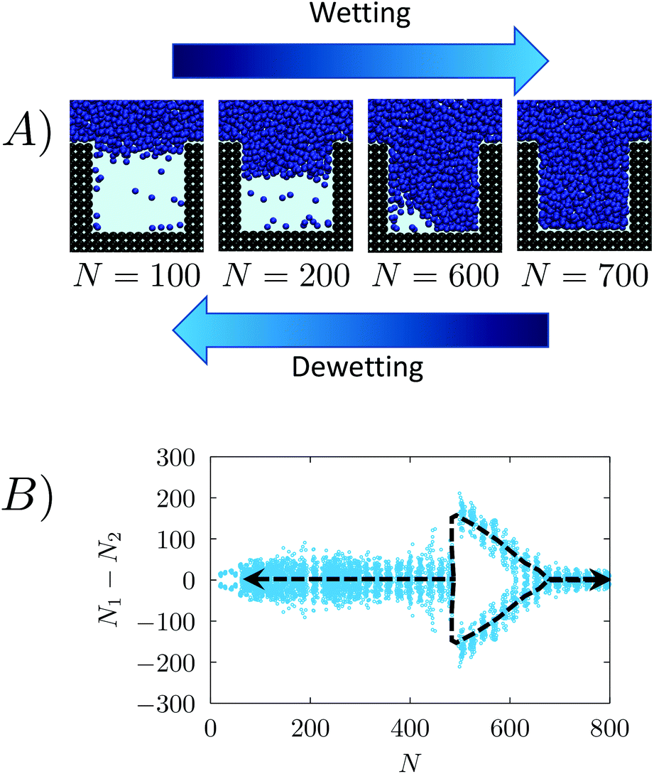
In addition to the Cassie–Baxter state a second state exists, known as the Wenzel state,17 in which the liquid completely wets the corrugations of the hydrophobic surface. In the Wenzel state the liquid/solid contact area is much larger and the superhydrophobic properties are lost. The Cassie–Baxter/Wenzel transition (wetting – Fig. 1) can be induced by changes of pressure and/or temperature.18,19 The fragility of the Cassie–Baxter state and the difficulty of recovery (Wenzel/Cassie–Baxter transition20–22) have hindered the use of superhydrophobic surfaces in practical applications. Thus, intense experimental and theoretical research has been devoted to the investigation of the wetting and recovery mechanisms.20,22–38
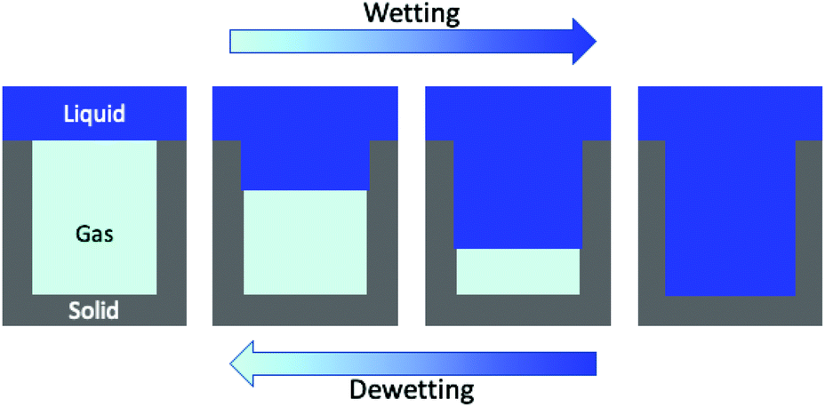 | ||
| Fig. 1 Cartoon of the wetting (left-to-right) and recovery (right-to-left) paths. | ||
In their seminal work, Lafuma and Quéré22 have investigated the variation of the contact angle hysteresis as a function of the pressure of a liquid droplet deposited between two textured hydrophobic surfaces. A large and sudden increase of the contact angle hysteresis is a measure of the transition from the Cassie–Baxter to the Wenzel state. In particular, Lafuma and Quéré have shown that upon relaxing the pressure the contact angle hysteresis does not recover the original value; that is, the transition is irreversible.
The experimental investigation of the wetting mechanism in submerged surfaces poses challenges for following the evolution of the state of the system with the change of external conditions. Optical techniques have been employed for this purpose, such as light reflection stereo microscopy (see, e.g., ref. 39) and transmission diffraction (see, e.g., ref. 20, 40 and 41). In contrast with these indirect techniques, confocal microscopy directly follows the evolution of the liquid–air meniscus,24,42,43 which makes it an optimal tool for investigating the wetting and recovery mechanism. In particular, Duan and coworkers used confocal microscopy to follow the evolution of the water meniscus while the pressurized liquid enters into the cylindrical pores decorating a hydrophobic surface.24,43 They have shown that water intrudes the pores with a symmetric, almost flat, meniscus. Indeed, also an asymmetric wetting path has been observed in these experiments, which consists in the formation of a gas bubble at the bottom of corrugations which is then absorbed. The observation of this second wetting path has been attributed to the presence of impurities accumulating on the side walls of corrugations that pin the meniscus during its advancement.
Under the conditions of interest for experiments and technological applications the wetting and recovery transitions are often characterized by (relatively) large free-energy barriers (ΔΩ†w and ΔΩ†r, respectively) separating the initial and final states. In the presence of barriers larger than the thermal energy kBT (kB Boltzmann constant and T temperature) the transition time scales exponentially with ΔΩ†w/r:44,45
| τw/r = τ0w/r exp(ΔΩ†w/r/kBT). | (1) |
Because of this long transition time, largely exceeding the timescale accessible to brute force (continuum and/or atomistic) simulations, special techniques are necessary to investigate the wetting and recovery transitions. Apart from notable exceptions,46,47 the wetting and recovery of textured surfaces has been studied via quasi-static methods, such as umbrella sampling,31 restrained molecular dynamics,27,37,48 string and nudged elastic band methods.32,33,36,48–51 These methods assume that the process is slow and the system is at the local equilibrium all along wetting or recovery. In other words, these methods neglect dynamic effects, such as inertia. For a set of textured surfaces, e.g. surfaces with circular and square pores, ridges and pillars, the most probable wetting path predicted by quasi-static approaches – the one associated with the lowest free-energy barrier – breaks the symmetry of the system; for example, it is characterized by the formation of a gas bubble in the corner of the corrugations.27–29,48,52 The comparison with complementary quasi-static macroscopic theories and simulations28,32 confirms that the characteristic length of surface corrugations does not alter the overall picture of the wetting mechanism, which remains asymmetric. These results confirm that quasi-static theoretical predictions are at odds with the recent experiments discussed above.
The objective of this work is to reconcile the mismatch between theory and experiments, i.e. to identify the neglected terms that are responsible for the symmetric wetting and to extend existing theories to predict a wetting path consistent with experimental observations. This extended framework is expected to be relevant also for related phenomena, such as homogeneous and heterogeneous bubble nucleation, which hardly conforms to a quasi-static picture.53,54 To achieve our aim we perform molecular dynamics (MD) simulations that, as discussed in more detail in the next section, embodies all relevant phenomena affecting the evolution of the solid–liquid–gas three phase system. The use of atomistic simulations, however, imposes some constraint on the size of textures that can be simulated, between 1 and 10 nm. Nevertheless, as discussed in more detail in the next section, fluid mechanics arguments based on dimensionless numbers, namely the Womersley number, confirm that our conclusions can be extended to larger textures of experimental and applicative interest.
We investigate a wide range of thermodynamic conditions. In particular, we run simulations at pressures corresponding to high and low wetting barriers associated, respectively, with long and short transition times. The former corresponds to ambient conditions, of practical interest for most of the common textured hydrophobic surfaces, and the latter to more extreme conditions used in wetting experiments.
The present results are of interest from both the fundamental and the application points of view: in addition to revealing paramount dynamic effects in nucleation, such a theory opens a way to design surfaces with tailored properties that can better resist wetting32,55,56 and enable facile recovery.31,52 Similar dynamic effects are expected to play a role in the broader context of heterogeneous nucleation, liquid fronts moving on actual surfaces, self-assembly, micelle formation, etc. Moreover, wetting and recovery, liquid intrusion in and extrusion from lyophobic pores, is important for the emerging field of mechanical energy storage and energy dissipation using nanometric hydrophobic porous systems, such as mesoporous silica, e.g. MCM-4157 (pore size ∼2–6.5 nm), or metal–organic frameworks (MOFs), e.g. ZIF-858,59 (pore size ∼1.2 nm).
We remark that our simulations allow reconciling the experimental and theoretical pictures of wetting: when the free-energy barrier is sufficiently low – close to the values at which the experimental transition is expected to occur – dynamic effects dominate and the meniscus advances inertially in the pores, preserving the initial symmetric shape. In addition, our results support the interpretation that the asymmetric wetting observed from time to time in experiments is due to the deposition of impurities on the textured walls. Finally, in contrast with the quasi-static picture,28,31–33,36,37,48,50,51 the present results show that dynamic effects are strongly dependent on the liquid pressure.
Results and discussion
We investigated the wetting and recovery by the atomistic simulations summarized below and described it in more detail in the Methods section. The advantage of atomistic simulations is that all the complex and, possibly, relevant properties and phenomena, e.g. line and surface tension, and their dependence on the meniscus curvature during wetting/recovery, are consistently contained in the interaction potential between the fluid and solid particles. As anticipated in the Introduction, apart from notable exceptions,34 the wetting and recovery has been investigated at a theoretical level using quasi-static approaches, such as suitable extensions of the classical nucleation theory (CNT28), umbrella sampling (US31), restrained molecular dynamics (RMD27) or analogous techniques. In quasi-static methods one acts as a Maxwell daemon increasing or decreasing the level of filling of the pore (Fig. 1) starting from the empty (wetting) or completely filled pore (recovery). At each level of filling one computes the properties of the system, including its (conditional) distribution and energetics. It must be remarked that under quasi-static conditions the process is reversible and the recovery path is just the reverse of the wetting one.48In the present work we use RMD to provide (quasi-static) reference results for comparison. Here, we control (restrain) the number of fluid particles in the pore N (Fig. 2A). A continuum fluid dynamics analysis (Navier–Stokes equations60) may help understanding the limitations of quasi-static approaches. In atomistic simulations the wetting/recovery liquid velocity can be recast into the form u = mṄ/(Aρ), where Ṅ is liquid particles’ wetting/recovery rate, A is the area of the pore, and m and ρ are the particle mass and the liquid density, respectively. In quasi-static approaches Ṅ is set to 0 by the restraint at any point along the process and so is the liquid velocity u. This amounts to neglecting inertial over viscous forces, as quantified by the Womersley number
| α2 = 2π Sr Re = ρL2/μτ = mṄ/μL = 0, | (2) |
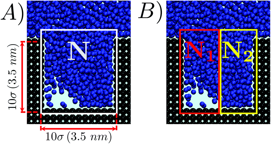 | ||
| Fig. 2 (A) Computational sample used in the simulations. The blue and brown spheres represent the fluid and solid particles, respectively. The order parameter N(r) is the number of particles within the white frame. (B) The red and yellow frames define the boxes used to determine N1 and N2 for the calculation of ΔN = N1(r) − N2(r). | ||
Our FFS simulations show that, when wetting and recovery take place on the experimental timescale, α2 reaches values up to 0.33 (see below), suggesting that inertia may play an important role in modeling these processes. We remark that, when dimensionless numbers are invaluable to quantify inertial effects, (mean-field) Navier–Stokes equations cannot be used to simulate thermally activated processes, where thermal fluctuations are the key to overcome free-energy barriers. The atomistic simulations discussed in the following incorporate such thermal fluctuations and enabled us to assess the relevance of inertia in the wetting/recovery process under varying thermodynamic conditions – specifically liquid pressure.
We first consider a Lennard–Jones (LJ) liquid wetting a surface made of LJ particles and featuring a 10 × 10 ridge (∼3.5 nm × 3.5 nm if the liquid were water), i.e. a square cavity extending infinitely in the direction orthogonal to the plane of Fig. 1. This geometry has been extensively investigated in previous theoretical28,38,61,62 and computational27,30,48 studies because despite its simplicity it embodies all the ingredients governing the wetting/recovery transition.61 The fluid and solid particles interact via the modified LJ potential
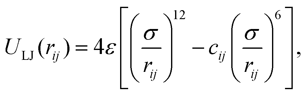 | (3) |
We performed RMD simulations, i.e. without inertia, of the wetting and recovery processes at different liquid pressures, corresponding to different values of the free energy difference ΔΩCB/W between the Cassie–Baxter and Wenzel states and of the wetting/recovery barrier ΔΩ†w/r: higher pressures favor the stability of the Wenzel state and reduce the wetting barrier and vice versa (see Fig. 3 and Table 1). In particular, at P = −0.168 and P = −0.08 Cassie–Baxter is the stable state and Wenzel is the metastable one; the situation is reversed at P = −0.005, 0.01, and 0.035: Wenzel is the stable state and Cassie–Baxter is the metastable one. According to eqn (1), only when the barrier is of the order of few kBT does the transition take place on the experimental timescale (milliseconds to seconds). Thus, considering the wetting and recovery barriers reported in the table, our RMD results suggest that, among the pressures considered, wetting readily takes place at P = 0.035 and recovery at P = −0.168.
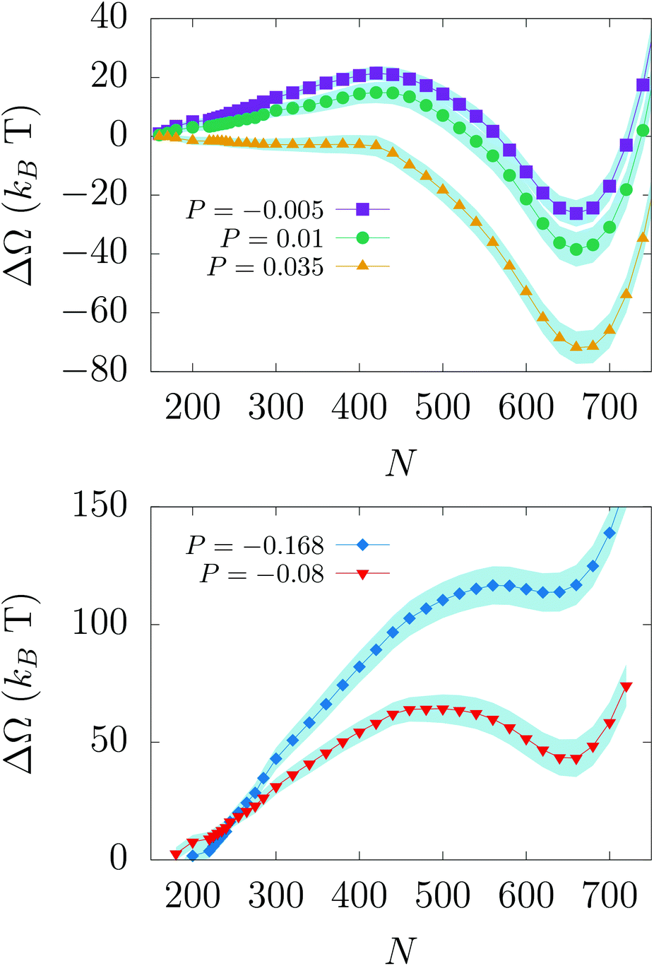 | ||
| Fig. 3 Free energy profiles as a function of the number of particles inside the pore computed via RMD at various pressures. The Cassie–Baxter state is at N ≈ 200, while the Wenzel one is at N ≈ 700. The shadow regions beneath the symbols represent the error on the free energy, namely three times the standard deviation of ΔΩ (see the Methods section for technical details). An arbitrary constant is added to the free energy so that ΔΩ = 0 at the Cassie–Baxter state. | ||
| P | ΔΩCB/W | ΔΩ†w | ΔΩ†r |
|---|---|---|---|
| -0.168 (−3.8) | −130 | 133 | 3 |
| -0.08 (−1.8) | -74 | 91 | 17 |
| -0.005 (−0.1) | 21 | 17 | 38 |
| 0.01 (0.2) | 31 | 12 | 43 |
| 0.035 (0.8) | 57 | 0 | 57 |
Consistent with literature results,27,28,32 the RMD wetting transition begins with liquid depinning from the top corners and entering in the cavity with an (almost) flat meniscus (see Fig. 4A); in correspondence of the transition state (the maximum of the free-energy profile, N ∼ 450) the meniscus bends to form a vapor bubble in one of the two bottom corners of the cavity. Then, the bubble shrinks until it disappears when the system reaches the Wenzel state.
 | ||
| Fig. 4 (A) Sequence of snapshots along the wetting (left-to-right) and recovery (right-to-left) paths as obtained by restrained molecular dynamics.27,37,69 During the wetting the liquid initially enters in the pore with a flat meniscus, and then forms a bubble in a corner and finally the bubble is absorbed and the meniscus touches the bottom wall. The quasi-static process is reversible and thus the recovery path is the reverse of the wetting path. (B) Pairs of (ΔN, N) values sampled in RMD simulations of the wetting/recovery process at P = −0.08. Analogous graphs for the other pressures are shown in Fig. SM2.† The black dashed line, introduced to help the reader to follow the wetting/recovery path, is obtained by connecting the average value of ΔN at each N, 〈ΔN〉N; in the region in which the graph is split into two parts (N > 450) 〈ΔN〉N is computed within the domain of each mode. Consistent with the snapshots of panel (A), in the early part of the wetting ΔN values are concentrated about 0. At N ∼ 450 one observes a sharp change, with sizably negative and positive ΔN values. | ||
A more quantitative determination of the asymmetry of the liquid front along the wetting process is provided by ΔN = N1 − N2vs. N, where N1 and N2 are the numbers of liquid particles in the left and right halves of the cavity, respectively (Fig. 2B). When the meniscus is flat ΔN ∼ 0, and when a bubble is formed in a corner ΔN is either sizably negative or positive. The graph ΔN vs N for RMD is shown in Fig. 4B. Here we report the values of ΔN sampled at various N in RMD simulations at P = −0.08. The black dashed line, introduced to help the reader to follow the wetting/recovery path, is obtained by connecting the average values of ΔN at each N, 〈ΔN〉N; in the region in which the graph is split into two parts (N > 450) 〈ΔN〉N is computed within the domain of each mode. One notices that the wetting starts (low N) with a symmetric meniscus (ΔN is concentrated about 0). Then, in correspondence of the transition state, the system follows either the bubble-in-the-left (ΔN ≫ 0) or bubble-in-the-right (ΔN ≪ 0) corner paths. With the progress of the wetting process the bubble is absorbed and ΔN tends again to zero. Within the quasi-static approximation, the recovery path is just the reverse of the wetting one, as indicated by the arrows at both ends of the dashed line in Fig. 4B. The ΔN vs. N plots at the different pressures (Fig. SM2†) overlap, indicating that the wetting path is independent of the pressure triggering the process, as predicted by continuum theories of wetting.28
The same analysis is performed on the FFS simulations. In Fig. 5A–C is reported the probability m(ΔN, N) along the wetting at P = −0.005, 0.01 and 0.035. This figure is the FFS analogue of Fig. 4B, representing the probability to observe a value of ΔN at a given level of progress of the wetting as measured by N. One immediately notices that, at a variance with RMD, in this case the wetting path depends on the pressure: the m(ΔN, N) probabilities at different P are sizably different. Like in RMD, at low and moderate liquid pressures (panels A and B) the trajectories are initially (N ≤ 450) symmetric, with m(ΔN, N) concentrated about at ΔN = 0. Then, m(ΔN, N) splits into two branches corresponding to the bubble-in-the-left and bubble-in-the-right corner configurations. At P = 0.035, however, m(ΔN, N) is concentrated about zero all along the process, indicating that at high pressures the mechanism becomes symmetric (Fig. 5C).
 | ||
| Fig. 5 Logarithm of the probability density, log[m(ΔN,N)], along the wetting (A–C) and recovery (D–F) trajectories at different pressures. We refrain from using the same representation of Fig. 4 to highlight that while for RMD one refers to the equilibrium distribution data for FFS obtained by sampling ΔN at prescribed values of N along reactive trajectories. As in the case of Fig. 4, the black dashed line obtained from 〈ΔN〉N is introduced to guide the eye of the reader. At low (P = −0.005) and moderate (P = 0.01) pressures the wetting follows a path consistent with the quasi-static picture of panel D. At higher pressures (P = 0.035) m(ΔN, N) is concentrated about ΔN = 0 all along the wetting path. The recovery always follows a path characterized by initial (N > 400) large positive or negative values of ΔN. However, at small and moderate negative pressures (P = −0.005, −0.08) in the second part of the path (N < 400 and N < 200, respectively) m(ΔN, N) is concentrated about 0, indicating a recovery of the symmetrical morphology of the meniscus. At P = −0.08 we observe multiple transition channels, as highlighted by multiple dashed lines in the central part of the process, between N = 500 and 200. At more negative pressures (P = −0.168) m(ΔN, N) remains centered at large negative or positive values all along the recovery. | ||
The discrepancies between FFS and RMD suggest that inertia, neglected in the latter approach, plays a crucial role in the wetting of the cavity when the corresponding barrier is low, i.e. when the pressure is high: under these pressure conditions the thermodynamic and viscous forces are insufficient to change the shape of the liquid/gas interface to the minimum free-energy morphology. This claim is supported by the observation that the velocity of advancement of the meniscus, measured by Ṅ, significantly increases with the liquid pressure in correspondence of the transition state. This, indeed, is reflected on the doubling of the Womersley number with pressure, which goes from α2 ∼ 0.035 at P = −0.005 and 0.01 to α2 ∼ 0.07 at P = 0.035.70 In contrast, we observe no significant change of the velocity of bending of the meniscus, estimated by ΔṄ, with P (Fig. 6).
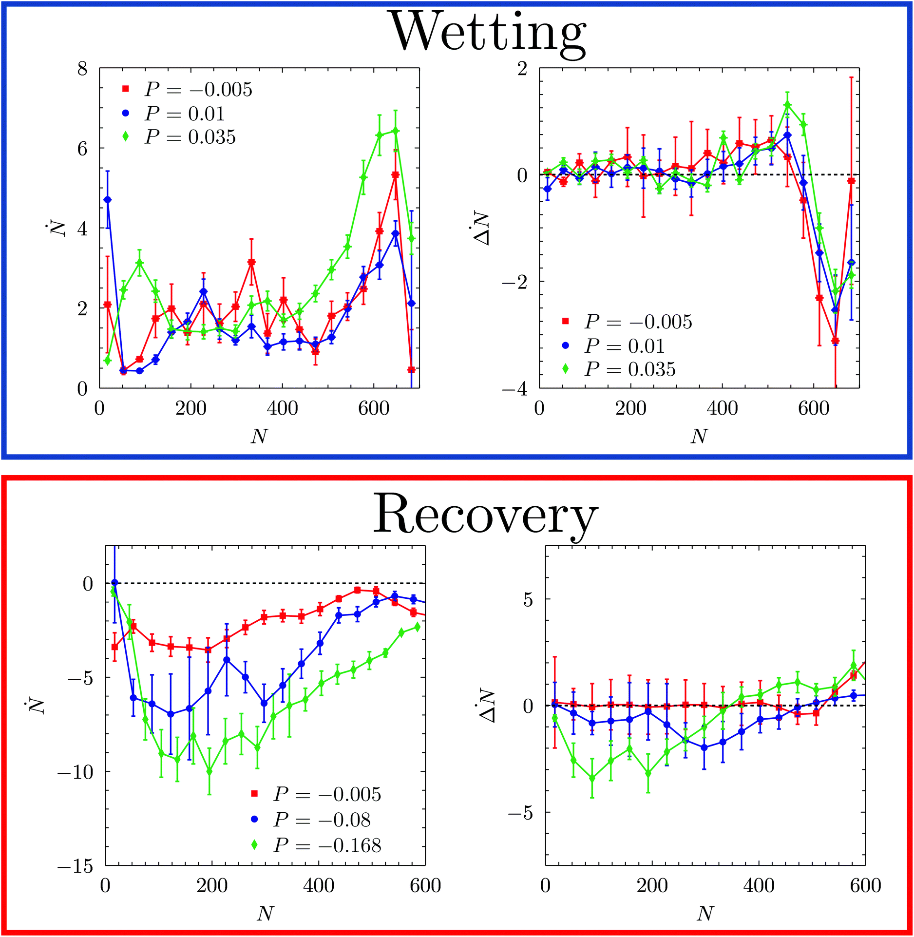 | ||
Fig. 6
Ṅ (left) and  (right) as a function of N. Ṅ measures the velocity of advancement of the liquid in the pore and (right) as a function of N. Ṅ measures the velocity of advancement of the liquid in the pore and  , the velocity of sloshing of the liquid from one half box to the other, measures the velocity of bending of the meniscus. In the top and bottom rows we report data for wetting and recovery, respectively. The dashed line representing zero velocity is reported when necessary. , the velocity of sloshing of the liquid from one half box to the other, measures the velocity of bending of the meniscus. In the top and bottom rows we report data for wetting and recovery, respectively. The dashed line representing zero velocity is reported when necessary. | ||
One question arises: to what extent the phenomena we observed on the 10 × 10 (3.5 nm × 3.5 nm) texture are relevant to experimentally accessible lateral scales, ∼10 nm (ref. 15 and 16) or more? As a first, empirical, confirmation that the same phenomena are relevant also on larger scales, we show that the transition from the asymmetric to symmetric path when pressure increases from −0.005 to P = 0.035 is also observed for a 20 × 20 pore (∼7 nm × 7 nm, – see Fig. SI1†). Concerning larger, macroscopic, corrugations, continuum fluid dynamics predicts that the relevance of inertia grows with the characteristic length of corrugation, as shown by the quadratic dependence of the Womersley number α2 = ρL2/μτ on the cavity mouth L. Thus, one expects that the role of inertia in the intrusion mechanism becomes more relevant for larger corrugations.
The present results for the nanoscopic corrugations – the relation between the wetting mechanism, asymmetric or symmetric, and the corresponding barrier – allow us to interpret recent experimental results of Duan and coworkers,24,38 which conflict with well established (macroscopic) quasi-static theories. Present results show that inertia induces a change in the wetting mechanism from asymmetric when the barrier is sizably larger than the thermal energy to symmetric when the barrier is small. At the same time, one expects that in experiments wetting is observed when the barrier is low as under these conditions the wetting time is within the experimental timescale (see eqn (1) and the corresponding discussion). Thus, we conclude that the symmetric wetting mechanism observed in experiments are driven by inertial effects, which are neglected in standard wetting theories. In other words, the inclusion of inertia allows one to reconcile the mismatch between theory and experiments.
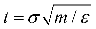
These conclusions are qualitatively confirmed considering the transition time τ of FFS wetting simulations (eqn (11)). Indeed, at low and moderate pressures, P = −0.05 and 0.01, corresponding to asymmetric wetting paths, the transition time is 1.5 × 10¹⁹ s (∼5 × 10¹¹ years) and 1.5 × 10⁸ s (∼5 years), respectively, well beyond the typical experimental time (microseconds to minutes). In contrast, at high pressure, P = 0.035, at which the transition path is symmetric, the transition time is rather short, 1.5 × 10⁻⁸ s (∼15 ns). Transition times in natural units (NU) have been obtained using the standard conversion relation  where m is the mass of a water molecule, and ε and σ the Lennard-Jones parameters of the TIP4P2005 water model,71 one of the most widely used water models (see Note72 for additional information). We remark that τNU is purely indicative and one should refrain from performing a quantitative comparison between experimental wetting times and transition times in natural units. There are several reasons for this, among which we recall that while in experiments the system (typically) contains air, our computational sample is completely degassed. This does not affect the wetting path37 but sizably reduces the transition time in simulations with respect to experiments as there is no air that must diffuse into the intruding water for the completion of the process. Here, an important observation is that, consistent with experiments, when the transition time is within the experimental timescale the wetting mechanism is symmetric.
We remark that at the highest pressure, the one at which the transition time is within the experimental timescale, the wetting follows only the symmetric path. This suggests that there is only one wetting channel active at a time, which supports the conclusion of Duan and coworkers24 that there must be an external agent, e.g. accumulation of impurities on the textured walls, inducing the system to follow the asymmetric wetting. Indeed, impurities may pin the meniscus and prevent its symmetric advancing. The effect of impurities accumulating on surface textures on the wetting mechanism will be investigated in detail in a forthcoming study.
We now consider the recovery process by which vapor is formed within the pore and pushes the liquid back to the top of corrugation, restoring the Cassie–Baxter state. We remark that this process is equivalent to cavitation or bubble nucleation under confinement, which are important in many applications.19,73–76 Given the findings on the wetting path, a question naturally arises: do dynamic effects play an important role in the recovery path as well? To address this question we considered three negative liquid pressures (suction), P = −0.005, P = −0.08, and P = −0.168 corresponding to large, intermediate, and negligible free-energy barriers, respectively (Fig. 3 and Table 1). Fig. 5D–F show m(ΔN, N) along reactive recovery trajectories. One notices that in all cases the process is asymmetric and begins with the formation of a bubble in a corner. However, at moderately negative pressures, P = −0.005 and −0.08 – i.e., when the recovery barrier is large – after the transition state the system recovers the symmetric configuration, consistent with the quasi-static picture. Indeed, at P = −0.08 one observes multiple transition channels, as highlighted by multiple dashed lines in the central part of the process, between N = 500 and 200. These multiple transition channels represent different sizes (N) at which the bubble undergoes a transition from the bubble-in-the-corner to a flat morphology. At more negative pressures, instead, the interface becomes even more asymmetric, maintaining this morphology for most of the recovery path. Only when the meniscus pins to one of the corners at the top of the cavity, is the symmetric Cassie–Baxter state recovered. Similar to the wetting case, when the recovery barrier is negligible the velocity of the extruding liquid is too fast for the meniscus to reach the quasi-static configuration at the current level of recovery (Fig. 6). In other words, like in the case of wetting, when the recovery barrier is very low inertial effects dominate. This is confirmed by a sizable growth of the Womersley number at the maximum Ṅ, which passes from ∼0.2 to ∼0.33 for P going from −0.005 to −0.168.
The inertial effects discussed above cause deviations from other equilibrium properties. For example, along wetting and recovery the value of the contact angle and the curvature of the meniscus are different from the ones predicted by the Young and (generalized) Laplace28 equations respectively, describing the shape of a quasi-static liquid/gas interface. For the recovery, these effects are shown in Fig. 7. In FFS simulations at moderately negative pressures (P = −0.005) the contact angle θ at the two points of the meniscus are equal and very close to the Young value, θY = 102°, all along the process. The departure from θY for small vapor bubbles is due to the limited accuracy in the determination of θ under these conditions. In contrast, at P = −0.168, where inertial effects are large, for most of the recovery the values of θ at the two contact points are significantly different, and very different from θY. In particular, we observed a jump in the value of θ at the right contact point when the bubble detaches from the bottom wall (N ∼ 300). Also notice that the curvature of the meniscus when the recovery is almost complete (N ∼ 100) is opposite to the one predicted by the (generalized) Laplace equation.
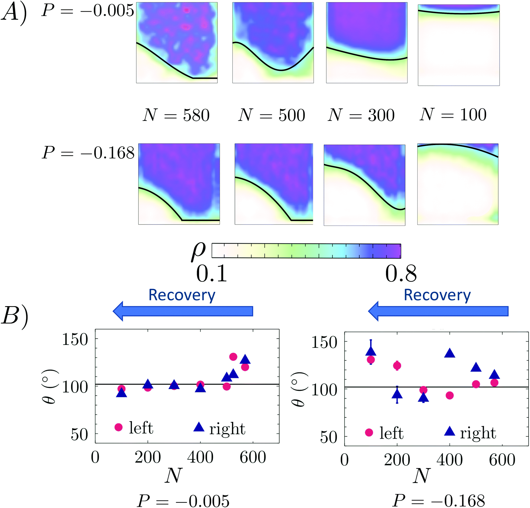 | ||
| Fig. 7 (A) Number density field of the fluid at selected points along the recovery process as obtained from FFS at P = −0.005 and −0.168. The density field is obtained by discretizing the pore in squared boxes and computing the contribution to the number of particles within each box from Gaussian distributions of standard deviation 1 centered at each particle position and, finally, dividing by the volume of the box. The Gibbs interface (black line) is obtained as a polynomial fitting of the points at mid density between the bulk liquid (violet) and bulk vapor (white). (B) Contact angle of the meniscus at the left and right liquid/vapor/solid contact points at P = −0.005 and −0.168. The contact angle is determined from the derivative of a polynomial interpolation of the liquid/vapor Gibbs interface at its intersect with the solid walls (Panel A). | ||
Conclusions
The present study has revealed that liquid inertia can determine important qualitative differences in wetting and recovery of rough surfaces, depending on the environmental conditions, e.g. the liquid pressure. In particular, it was found that by including inertia in the description of (thermally activated) wetting and recovery it is possible to reconcile experimental and theoretical results on the way in which a meniscus collapses in a pore. In particular, the symmetric wetting mechanism observed in present simulations under the conditions of a low wetting barrier is consistent with the recent confocal microscopy experiments of Duan and coworkers,24,25 which are also expected to be performed under the conditions of a low barrier, when wetting takes place on the experimental timescale (milliseconds to minutes).Contrary to previous quasi-static predictions, it was found that the wetting and recovery transition paths sensitively depend on the liquid pressure, underscoring the importance of liquid inertia. These dynamic effects play a crucial role also in enhancing the difference between the wetting and recovery processes, which are shown to follow symmetric and asymmetric paths, respectively, under typical experimental conditions.
We remark that the revealed phenomenology applies to a variety of physical phenomena well beyond wetting: condensation, cavitation, dynamics of the triple line, micelle formation and many more.
Our new predictions will hopefully stimulate the research community to perform accurate wetting and recovery experiments to identify the mechanism of the processes and their dependence on the thermodynamic conditions and on the direction of the path – wetting or recovery. For example, one could consider working with degassed water, which would help the comparison with simulations, which are typically performed with a pure liquid. Another important aspect to investigate experimentally is the difference between wetting and recovery: to the best of our knowledge, experiments addressing the recovery path are still lacking.
An interesting direction to pursue in the future is to assess the effect of heterogeneity and impurities on the wetting and recovery mechanism. Concerning theory, one could perform simulations on porous systems mimicking the presence of heterogeneities and/or the deposition of impurities on the texture walls.77 Complementarily, one could perform confocal microscopy experiments on systems containing an increasing content of impurities and determine whether the frequency of observation of the asymmetric mechanism has any relation with this.
The implication of present results for simulations is that, when the free-energy barriers characterizing a transition are low, it is crucial to include the dynamics beyond the quasi-static assumption common to many theories (e.g., classical nucleation theory) and rare event methods (e.g., umbrella sampling, restrained MD, string method, and nudged elastic band). From the practical point of view, this will help in developing more accurate strategies to design materials with tailored wetting and recovery properties78 beyond quasi-static theories and methods presently used.
Methods
Restrained molecular dynamics
The objective of the restrained molecular dynamics, RMD,69,79,80 is to sample the conditional density probability at a prescribed value of an observable, here the number of fluid particles in the pore, and the associated (Landau) free energy.81 The free energy Ω is defined as | (4) |
 . Within this approximation, the derivative of the free energy reads
 | (5) |
 | (6) |
In this work, we have set λ = 0.2, which has already been tested in previous studies to be a good trade-off between the convergence of dΩλ(N*)/dN with λ and the statistical error of the mean force (see, e.g., ref. 21, 55 and 82).
Assuming that the ensemble is at constant temperature, m(r)gλ(N(r) − N*) = exp(−β(V(r) + λ/2(N(r) − N*)2)), which can be sampled by a constant temperature MD driven by the augmented potential Ṽ(r;N*) = V(r) + λ/2(N(r) − N*)2, the so-called Restrained MD. Indeed, one can extend this approach to the isothermal-isobaric ensemble, provided that one uses molecular dynamics suitable to sample this ensemble.
In practice, dΩ(N*)/dN is computed as the time average of λ(N(r) − N*) along the RMD. Indeed, the conditional average of any observable can be computed as the time average of a suitable estimator along an RMD trajectory. We remark that RMD molecular dynamics is only used to sample the conditional ensemble; a single RMD trajectory does not represent the transition and its (fixed) duration bears no relation with the transition time.
Estimation of the free-energy error
Usually, the error on a derived observable O = O(s), with s the variable that is directly measured, is obtained by error propagation: | (7) |
 | (8) |
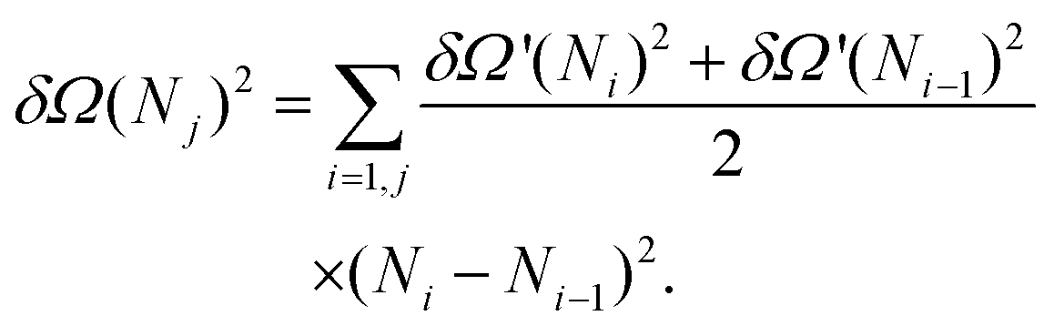
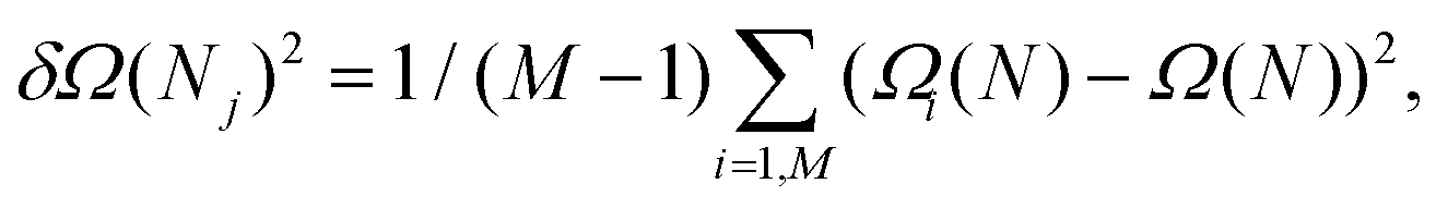
Here, like in previous studies,21,27,28,37,48,52,55,82,83 we use a different approach. We divide the 300![[thin space (1/6-em)]](https://www.rsc.org/images/entities/char_2009.gif) 000 configurations used to estimate dΩ(N)/dN into M smaller sets from which we obtain the corresponding estimates of the mean force {dΩi(N)/dN}i=1, M. From these, by numerical integration, one obtains a set of free energy curves Ωi(N)1=1, M that can be used to directly compute the variance δΩi(N)2 at each value of N:
000 configurations used to estimate dΩ(N)/dN into M smaller sets from which we obtain the corresponding estimates of the mean force {dΩi(N)/dN}i=1, M. From these, by numerical integration, one obtains a set of free energy curves Ωi(N)1=1, M that can be used to directly compute the variance δΩi(N)2 at each value of N:
 | (9) |
 is the free energy computed with the complete set of atomistic configurations. Then, one can obtain the error on Ω(N), taking properly into account correlation effects, using either the block average or the jackknife method.84
Forward flux sampling
Forward flux sampling (FFS85–88) is an algorithm that samples the ensemble of reactive trajectories from the reactant region A, e.g. the Cassie–Baxter state, to the product region B, the Wenzel state in this case. The progress of the transition is monitored by the value of an order parameter, the number of particles in the pore N(r) in this case. A set of l consecutive, non-intersecting interfaces is defined to partition the configuration space in regions. Such interfaces correspond to increasing values of {Ni(r)}i=0,l. The partitioning of the configuration space in domains delimited by these interfaces allows developing an algorithm, described in the following, that efficiently samples the improbable regions of the configuration space, e.g. the high free energy states near the transition state.The FFS algorithm consists of two steps. The first one evolves one (or more) trajectory initialized in the basin A and crossing the first interface N0. From this trajectory one can compute the flux Φ0 of MD trajectories crossing the boundary of the “reactant”. In the second step one evolves many trajectories starting from N0 and reaching either N1 or returning back to N0. From these trajectories one computes the conditional probabilities m(N1|N0) of reaching the next interface. The second step can be iterated for the other interfaces. The total rate of the A → B transition is finally evaluated according to the formula
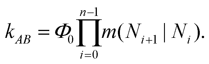 | (10) |
The transition time of the process is the inverse of the rate
| τ = 1/kAB. | (11) |
In addition, one obtains a sample of the ensemble of reactive trajectories under the prescribed thermodynamic conditions for the calculation of any statistical quantity along the reactive path.
The first step of the method requires the evolution of a (long) MD trajectory starting from the Cassie–Baxter state. The flux is computed as the number of positive crossings of the first interface, n0, divided by the total duration of the trajectory t
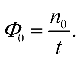 | (12) |
The hitting points of this trajectory with the first interface are used to initialize the second step of the algorithm. The hitting points with the second interface are used to initialize further trajectories aiming at the third interface and so forth. The ratio between the successful trajectories, nj+1, those hitting the next interface without returning to N0, and the total number of trajectories fired from the present one, n0j, gives the conditional probability m(Ni+1|Ni) = nj+1/n0j.
To have a statistical consistency, we run a fixed number of trajectories per interface, n0j = 544. Since the number of successful trajectories is lower than the number of fired ones, typically one has an insufficient number of different hitting points from which to start trajectories from the next interface. This problem can be addressed in several ways; here we use an approach in which one starts more than one trajectory from the same configuration. The stochastic dynamics prevents that two trajectories started from the same point overlap.
At a variance with RMD, FFS trajectories represent realistic reactive paths. The duration of these reactive trajectories decreases with the reduction of the barrier (Fig. SI3†). However, this is not the major effect of the barrier; what determines the reduction of the transition time is the increase of the number of reactive trajectories over the total number of attempted jumps from the initial to the final state. In fact, while the duration of the reactive branch of wetting and recovery trajectories, i.e. the part of the trajectory between depinning and complete wetting or vice versa, approximately halves over the range of pressures considered (Fig. SI3†), the transition time, which is the time one has to wait to observe a reactive event, including the time the system spends in the original basin, changes of 27 orders of magnitude.
Simulation details
The computational sample for both RMD and FFS simulations consisted of 68820 and 12790 fluid and solid particles, respectively. As explained above, liquid and solid particles interact via the modified LJ potential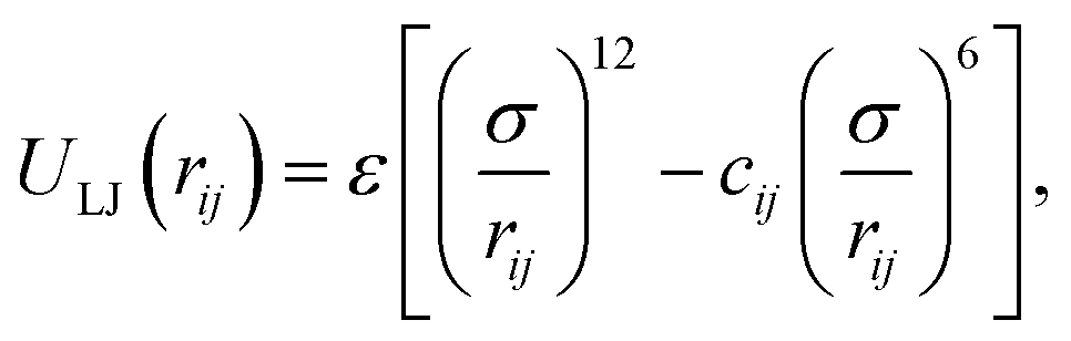 | (13) |
The parameter cij is set to 1 for fluid–fluid and solid–solid particle interactions. For fluid–solid interactions cij is set so that the contact angle θ takes a value close to 100°, typical of silanized or fluorinated surfaces.64–66 The value for cij is chosen following an iterative procedure consisting of three steps:27,55 (i) perform the simulation of a (cylindrical) droplet deposited on a flat surface with a guess value for cij, (ii) determine the value of the contact angle at the present value of cij, and (iii) adjust cij so as to increase/diminish the hydrophobicity of the surface.
The sample for the determination of the contact angle consisted of 54694 fluid and 70000 solid particles. Simulations were run in the NVT ensemble at the same temperature of the RMD and FFS simulations, T = 0.8. The drop (Fig. 8A) has a radius of ∼20. From the MD trajectory one determines the density field (Fig. 8B) and the (Gibbs) liquid/vapor dividing surface. This surface is fitted with a circumference and the contact angle is the derivative of the circumference at its contact point with the nominal position of the surface.
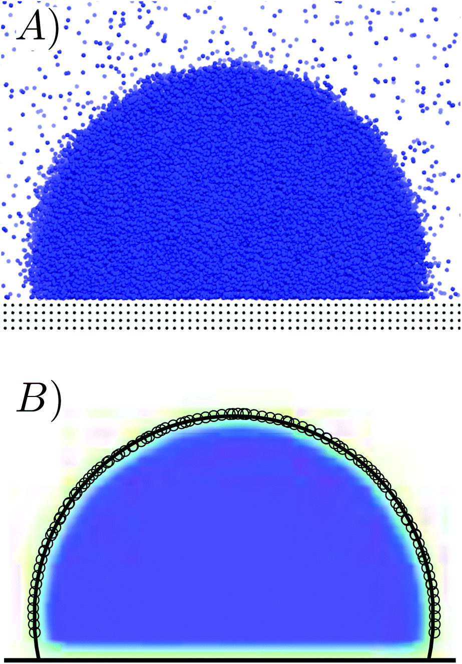 | ||
| Fig. 8 (A) snapshot of the atomistic droplet deposited on a solid surface. In panel (B) is shown the corresponding density field with the circumference fitting the (Gibbs) dividing liquid/vapor surface. | ||
RMD and FFS simulations were run at a constant number of particles, temperature and pressure (NPT ensemble) using the LAMMPS molecular dynamics code.89 Temperature was controlled using the Nosé-Hoover chain thermostat90 with a characteristic time of 0.1. Concerning the pressure, we have adopted the mechanical barostat recently introduced by Marchio et al.,91 which is suited for multi-phase systems. In practice, a solid slab of particles is added above the liquid and an extra force Fext = PA (P is the target pressure and A is the area of the solid slab) is applied to these particles. The time step for the numerical integration of the equation of motion was 0.005.
For RMD simulations we used 35 target values of the order parameter between N* = 160 and N* = 700. At each N* value we performed a 3 × 10⁵ step long RMD simulation.
The number of FFS interfaces is set such that the probability of reaching the next interface is 0.1 < m(Nj+1|Nj) < 0.5. The number of interfaces goes from 15 for the recovery process at very negative pressures to 50 for wetting at moderate pressure. The distance between interfaces varies along the path, going from a difference of 5 particles in the pore close to the transition state to 60 near the product state.
Conflicts of interest
There are no conflicts to declare.Acknowledgements
The research received funding from the European Research Council under the European Union's Seventh Framework Programme (FP7/2007–2013)/ERC grant agreement no. [339446]. This project has received funding from the European Research Council (ERC) under the European Union's Horizon 2020 research and innovation programme (grant agreement No 803213). SM acknowledges financial support from Sapienza University of Rome under the project “Porous Lyophobic Crystalline Materials for Mechanical Energy Storage”, grant. RG11715C81D4F43C. The authors acknowledge PRACE for awarding us access to resource Marconi based in Italy at Casalecchio di Reno. SM acknowledge the support of CINECA ISCRA-B for awarding the access to the FERMI supercomputer.References
- A. Cassie and S. Baxter, Trans. Faraday Soc., 1944, 40, 546–551 RSC.
- The Young and apparent contact angle of a liquid is the angle formed by the tangent to the droplet at contact point with the surface and the flat and textured surface itself. In the case of a textured surface, the nominal position of the surface is the plane passing by the top of the corrugations.
- The contact angle hysteresis is measured by the difference between the front and rear contact angles right before the droplet depins and slides/rolls along a tilted surface.
- The tilting angle is the maximum angle the surface can be tilted before the droplet deposited on it starts moving.
- M. Miwa, A. Nakajima, A. Fujishima, K. Hashimoto and T. Watanabe, Langmuir, 2000, 16, 5754–5760 CrossRef CAS.
- L. Feng, S. Li, Y. Li, H. Li, L. Zhang, J. Zhai, Y. Song, B. Liu, L. Jiang and D. Zhu, Adv. Mater., 2002, 14, 1857–1860 CrossRef CAS.
- X. Zhang, F. Shi, J. Niu, Y. Jiang and Z. Wang, J. Mater. Chem., 2008, 18, 621–633 RSC.
- M. Nosonovsky and B. Bhushan, Curr. Opin. Colloid Interface Sci., 2009, 14, 270–280 CrossRef CAS.
- J. E. Y. Jin, Y. Deng, W. Zuo, X. Zhao, D. Han, Q. Peng and Z. Zhang, Adv. Mater. Interfaces, 2017, 5, 1701052–1701039 Search PubMed.
- M. Zhang, S. Feng, L. Wang and Y. Zheng, Biotribology, 2016, 5, 31–43 CrossRef.
- L. Cao, A. K. Jones, V. K. Sikka, J. Wu and D. Gao, Langmuir, 2009, 25, 12444–12448 CrossRef CAS PubMed.
- J. A. Howarter and J. P. Youngblood, Macromol. Rapid Commun., 2008, 29, 455–466 CrossRef CAS.
- M. Ferrari and A. Benedetti, Adv. Colloid Interface Sci., 2015, 222, 291–304 CrossRef CAS PubMed.
- Y. Y. Yan, N. Gao and W. Barthlott, Adv. Colloid Interface Sci., 2011, 169, 80–105 CrossRef CAS PubMed.
- Y. K. Ryu Cho, C. D. Rawlings, H. Wolf, M. Spieser, S. Bisig, S. Reidt, M. Sousa, S. R. Khanal, T. D. Jacobs and A. W. Knoll, ACS Nano, 2017, 11, 11890–11897 CrossRef CAS PubMed.
- A. Checco, A. Rahman and C. T. Black, Adv. Mater., 2014, 26, 886–891 CrossRef CAS PubMed.
- R. N. Wenzel, Ind. Eng. Chem., 1936, 28, 988–994 CrossRef CAS.
- C. E. Brennen, Cavitation and bubble dynamics, Cambridge University Press, 2013 Search PubMed.
- A. R. Betz, J. Jenkins and D. Attinger, et al. , Int. J. Heat Mass Transfer, 2013, 57, 733–741 CrossRef CAS.
- A. Checco, B. M. Ocko, A. Rahman, C. T. Black, M. Tasinkevych, A. Giacomello and S. Dietrich, Phys. Rev. Lett., 2014, 112, 216101 CrossRef.
- M. Amabili, A. Giacomello, S. Meloni and C. M. Casciola, J. Phys.: Condens. Matter, 2016, 29, 014003 CrossRef PubMed.
- A. Lafuma and D. Quéré, Nat. Mater., 2003, 2, 457 CrossRef CAS PubMed.
- C. Lee and C.-J. Kim, Phys. Rev. Lett., 2011, 106, 014502 CrossRef PubMed.
- P. Lv, Y. Xue, H. Liu, Y. Shi, P. Xi, H. Lin and H. Duan, Langmuir, 2015, 31, 1248–1254 CrossRef CAS PubMed.
- Y. Xue, P. Lv, H. Lin and H. Duan, Appl. Mech. Rev., 2016, 68, 030803 CrossRef.
- Y. Wang, M. E. Zaytsev, H. L. The, J. C. Eijkel, H. J. Zandvliet, X. Zhang and D. Lohse, ACS Nano, 2017, 11, 2045–2051 CrossRef CAS PubMed.
- A. Giacomello, S. Meloni, M. Chinappi and C. M. Casciola, Langmuir, 2012, 28, 10764–10772 CrossRef CAS PubMed.
- A. Giacomello, M. Chinappi, S. Meloni and C. M. Casciola, Phys. Rev. Lett., 2012, 109, 226102 CrossRef PubMed.
- H. Kusumaatmaja, M. Blow, A. Dupuis and J. Yeomans, EPL, 2008, 81, 36003 CrossRef.
- R. J. Vrancken, H. Kusumaatmaja, K. Hermans, A. M. Prenen, O. Pierre-Louis, C. W. Bastiaansen and D. J. Broer, Langmuir, 2010, 26, 3335–3341 CrossRef CAS PubMed.
- S. Prakash, E. Xi and A. J. Patel, Proc. Natl. Acad. Sci. U. S. A., 2016, 113, 5508–5513 CrossRef CAS PubMed.
- J. R. Panter and H. Kusumaatmaja, J. Phys.: Condens. Matter, 2017, 29, 084001 CrossRef CAS PubMed.
- W. Ren, Langmuir, 2014, 30, 2879–2885 CrossRef CAS PubMed.
- E. S. Savoy and F. A. Escobedo, Langmuir, 2012, 28, 3412–3419 CrossRef CAS PubMed.
- Y. Li, D. Quéré, C. Lv and Q. Zheng, Proc. Natl. Acad. Sci. U. S. A., 2017, 114, 3387–3392 CrossRef CAS PubMed.
- G. Pashos, G. Kokkoris and A. G. Boudouvis, Langmuir, 2015, 31, 3059–3068 CrossRef CAS PubMed.
- A. Giacomello, M. Chinappi, S. Meloni and C. M. Casciola, Langmuir, 2013, 29, 14873–14884 CrossRef CAS PubMed.
- Y. Xiang, S. Huang, P. Lv, Y. Xue, Q. Su and H. Duan, Phys. Rev. Lett., 2017, 119, 134501 CrossRef PubMed.
- P. Forsberg, F. Nikolajeff and M. Karlsson, Soft Matter, 2011, 7, 104–109 RSC.
- L. Lei, H. Li, J. Shi and Y. Chen, Langmuir, 2009, 26, 3666–3669 CrossRef PubMed.
- A. Checco, T. Hofmann, E. DiMasi, C. T. Black and B. M. Ocko, Nano Lett., 2010, 10, 1354–1358 CrossRef CAS PubMed.
- P. Papadopoulos, L. Mammen, X. Deng, D. Vollmer and H.-J. Butt, Proc. Natl. Acad. Sci. U. S. A., 2013, 110, 3254–3258 CrossRef CAS PubMed.
- P. Lv, Y. Xue, Y. Shi, H. Lin and H. Duan, Phys. Rev. Lett., 2014, 112, 196101 CrossRef PubMed.
- H. Eyring, J. Chem. Phys., 1935, 3, 107–115 CrossRef CAS.
- R. Zwanzig, Nonequilibrium Statistical Mechanics, Oxford University Press, 2001 Search PubMed.
- E. S. Savoy and F. A. Escobedo, Langmuir, 2012, 28, 16080–16090 CrossRef CAS PubMed.
- J. Mo, J. Sha, D. Li, Z. Li and Y. Chen, Nanoscale, 2019, 11, 8408–8415 RSC.
- A. Giacomello, S. Meloni, M. Müller and C. Casciola, J. Chem. Phys., 2015, 142, 104701 CrossRef PubMed.
- W. Yao and W. Ren, J. Chem. Phys., 2015, 143, 244701 CrossRef PubMed.
- Y. Li and W. Ren, Langmuir, 2014, 30, 9567–9576 CrossRef CAS PubMed.
- G. Pashos, G. Kokkoris, A. Papathanasiou and A. Boudouvis, J. Chem. Phys., 2016, 144, 034105 CrossRef CAS PubMed.
- E. Lisi, M. Amabili, S. Meloni, A. Giacomello and C. M. Casciola, ACS Nano, 2018, 12, 359–367 CrossRef CAS PubMed.
- N. Bremond, M. Arora, C.-D. Ohl and D. Lohse, J. Phys.: Condens. Matter, 2005, 17, S3603 CrossRef CAS.
- G. Menzl, M. A. Gonzalez, P. Geiger, F. Caupin, J. L. Abascal, C. Valeriani and C. Dellago, Proc. Natl. Acad. Sci. U. S. A., 2016, 113, 13582–13587 CrossRef CAS PubMed.
- M. Amabili, A. Giacomello, S. Meloni and C. M. Casciola, Adv. Mater. Interfaces, 2015, 2, 1500248 CrossRef.
- A. Giacomello, L. Schimmele, S. Dietrich and M. Tasinkevych, Soft Matter, 2016, 12, 8927–8934 RSC.
- L. Guillemot, T. Biben, A. Galarneau, G. Vigier and É. Charlaix, Proc. Natl. Acad. Sci. U. S. A., 2012, 109, 19557–19562 CrossRef CAS PubMed.
- G. Ortiz, H. Nouali, C. Marichal, G. Chaplais and J. Patarin, Phys. Chem. Chem. Phys., 2013, 15, 4888–4891 RSC.
- Y. Grosu, S. Gomes, G. Renaudin, J.-P. E. Grolier, V. Eroshenko and J.-M. Nedelec, RSC Adv., 2015, 5, 89498–89502 RSC.
- G. K. Batchelor, An introduction to fluid dynamics, Cambridge University Press, 2009 Search PubMed.
- N. A. Patankar, Langmuir, 2004, 20, 7097–7102 CrossRef CAS PubMed.
- N. A. Patankar, Langmuir, 2010, 26, 8941–8945 CrossRef CAS PubMed.
- Chart of the joint probability ΔN vs. N for the larger 20 × 20 pore and quasi-static data for the five different pressures available in the ESI.†.
- W. Chen, A. Y. Fadeev, M. C. Hsieh, D. Öner, J. Youngblood and T. J. McCarthy, Langmuir, 1999, 15, 3395–3399 CrossRef CAS.
- D. Öner and T. J. McCarthy, Langmuir, 2000, 16, 7777–7782 CrossRef.
- J. W. Grate, K. J. Dehoff, M. G. Warner, J. W. Pittman, T. W. Wietsma, C. Zhang and M. Oostrom, Langmuir, 2012, 28, 7182–7188 CrossRef CAS PubMed.
- It is worth remarking that the definition of the size of the cavity mouth L of an atomistic system poses problems. Here we use the distance between atoms of the opposite walls; however, this does not correspond to the space available to the liquid as between the solid and liquid particles exists a so-called depletion zone. The length of this zone depends on the contact angle θY but its typical value is ∼1σ. In macroscopic systems the size of the depletion zone is negligible with respect to the cavity mouth; on the contrary, in nanoscopic systems the depletion zone might be a sizable fraction of L, here ∼20%.
- Consistent with the macroscopic value of the intrusion pressure, Pint = −2cos(θY)γ/L = 0.018, the barrier at P = 0.035 is zero. However, the estimate of the intrusion pressure of a nanoscopic system according to macroscopic equations poses problems. In addition to the definition of the cavity mouth discussed in the note,67 the estimate of the contact angle by atomistic simulations can be inaccurate for several reasons. Here we recall that the identification of the position of the liquid/gas interface to define the tangent to the bubble and the position of the solid interface against which to compute the contact angle is not unique: slightly differences in the (arbitrary) positioning of these interfaces/surfaces in atomic systems (see Fig. 8) brings to changes in the estimation of θY.
- L. Maragliano and E. Vanden-Eijnden, Chem. Phys. Lett., 2006, 426, 168–175 CrossRef CAS.
- For the calculation of the Womersley number we used m = 1, as in the simulations, L = 10, corresponding to the hight of the cavity, and μ = 3, as reported in the literature.92Ṅ is measured in correspondence of the transition state, where one observes the break of symmetry with the formation of the bubble-in-the-left and bubble-in-the-right meniscus morphology in the RMD simulations.
- J. L. Abascal and C. Vega, J. Chem. Phys., 2005, 123, 234505 CrossRef CAS PubMed.
- The transformation of physical quantities from Lennard–Jones into SI units follows a standard procedure stemming from the definition of fundamental
(mass, m, length, σ, and energy, ε) and derived (time,
 , pressure, P = ε/σ3) LJ units. Given a transition time in LJ units, τLJ, one obtains the corresponding values in natural – SI – units by the standard relation
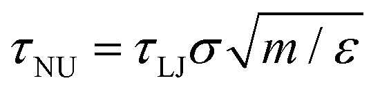
  . Here, m, ε and σ are the value of the water molecular mass, LJ characteristic energy and length in grams, joules and meters, respectively. These quantities are available in standard force fields. Here we use values of the TIP4P2005 water model:71m = 2.9915 × 10⁻²⁶ kg, ε = 1.28867 × 10⁻²¹ m2 kg s−2 and σ = 3.1589 × 10⁻¹⁰ m. Thus, τNU∼ 1.5 × 10⁻¹¹τLJ.
 - E. A. Neppiras, Phys. Rep., 1980, 61, 159–251 CrossRef.
- J. R. Blake and D. Gibson, Annu. Rev. Fluid Mech., 1987, 19, 99–123 CrossRef.
- K. S. Suslick, Y. Didenko, M. M. Fang, T. Hyeon, K. J. Kolbeck, W. B. McNamara, M. M. Mdleleni and M. Wong, Philos. Trans. R. Soc., A, 1999, 357, 335–353 CrossRef CAS.
- C. C. Coussios and R. A. Roy, Annu. Rev. Fluid Mech., 2008, 40, 395–420 CrossRef.
- A. Giacomello, L. Schimmele and S. Dietrich, Proc. Natl. Acad. Sci. U. S. A., 2016, 113, E262–E271 CrossRef CAS PubMed.
- J. Panter, Y. Gizaw and H. Kusumaatmaja, Sci. Adv., 2019, 5, eaav7328 CrossRef CAS PubMed.
- G. Ciccotti and S. Meloni, Phys. Chem. Chem. Phys., 2011, 13, 5952–5959 RSC.
- S. Meloni and G. Ciccotti, Eur. Phys. J.: Spec. Top., 2015, 224, 2389–2407 CAS.
- S. Bonella, S. Meloni and G. Ciccotti, Eur. Phys. J. B, 2012, 85, 97 CrossRef CAS.
- M. Amabili, S. Meloni, A. Giacomello and C. M. Casciola, J. Phys. Chem. B, 2017, 122, 200–212 CrossRef PubMed.
- M. Amabili, A. Giacomello, S. Meloni and C. M. Casciola, Phys. Rev. Fluids, 2017, 2, 034202 CrossRef.
- W. Janke, Quantum Simulations of Complex Many-Body Systems: From Theory to Algorithms, 2002, vol. 10, pp. 423–445 Search PubMed.
- R. J. Allen, P. B. Warren and P. R. ten Wolde, Phys. Rev. Lett., 2005, 94, 018104 CrossRef PubMed.
- R. J. Allen, D. Frenkel and P. R. ten Wolde, J. Phys. Chem., 2006, 124, 024102 CrossRef PubMed.
- C. Valeriani, R. J. Allen, M. J. Morelli, D. Frenkel and P. R. Rein ten Wolde, J. Chem. Phys., 2007, 127, 114109 CrossRef PubMed.
- R. J. Allen, C. Valeriani and P. R. ten Wolde, J. Phys.: Condens. Matter, 2009, 21, 463102 CrossRef PubMed.
- S. Plimpton, J. Comput. Phys., 1995, 117, 1–19 CrossRef CAS.
- G. J. Martyna, M. L. Klein and M. Tuckerman, J. Chem. Phys., 1992, 97, 2635 CrossRef.
- S. Marchio, S. Meloni, A. Giacomello and C. M. Casciola, J. Chem. Phys., 2018, 148, 064706 CrossRef CAS PubMed.
- K. Meier, A. Laesecke and S. Kabelac, J. Chem. Phys., 2004, 121, 9526–9535 CrossRef CAS PubMed.
Footnote |
| † Electronic supplementary information (ESI) available: Bubble morphology for larger pores and at various pressures. See DOI: 10.1039/c9nr05105h |
| This journal is © The Royal Society of Chemistry 2019 |