
 Open Access Article
 This Open Access Article is licensed under a Creative Commons Attribution-Non Commercial 3.0 Unported Licence
Fast, quantitative and high resolution mapping of viscoelastic properties with bimodal AFM†
Simone
Benaglia
,
Carlos A.
Amo
and
Ricardo
Garcia
 *
*
Material Science Factory, Instituto de Ciencia de Materiales de Madrid, CSIC, c/Sor Juana Ines de la Cruz 3, 28049 Madrid, Spain. E-mail: r.garcia@csic.es
First published on 6th August 2019
Abstract
Quantitative mapping of viscoelastic properties of soft matter with a nanoscale spatial resolution is an active and relevant research topic in atomic force microscopy (AFM) and nanoscale science characterization. The AFM has demonstrated its accuracy to measure the energy dissipated on a sample surface with an atomic-scale resolution. However, the transformation of energy dissipation values associated with viscoelastic interactions to a material property remains very challenging. A key issue is to establish the relationship between the AFM observables and some material properties such as viscosity coefficient or relaxation time. Another relevant issue is to determine the accuracy of the measurements. We demonstrate that bimodal atomic force microscopy enables the accurate measurement of several viscoelastic parameters such as the Young's modulus, viscosity coefficient, retardation time or loss tangent. The parameters mentioned above are measured at the same time that the true topography. We demonstrate that the loss tangent is proportional to the viscosity coefficient. We show that the mapping of viscoelastic properties neither degrades the spatial resolution nor the imaging speed of AFM. The results are presented for homogeneous polymer and block co-polymer samples with Young's modulus, viscosity and retardation times ranging from 100 MPa to 3 GPa, 10 to 400 Pa s and 50 to 400 ns, respectively. Numerical simulations validate the accuracy of bimodal AFM to determine the viscoelastic parameters.
1. Introduction
The understanding, characterization and mapping of the viscoelastic properties of soft matter at the nanoscale level is an active area of research in polymer science, nanolithography, mechanobiology and force microscopy.1–12 The development of novel nanolithographies demands a fast and high resolution characterization of the viscoelastic properties of polymer resists.12,13 In mechanobiology, there is some evidence that supports the influence of the cell's viscoelastic processes in its physiology.14–17 However, the interpretation of the AFM data in terms of the viscoelastic parameters of the sample is quite challenging. Among other issues, there is no established and generally accepted framework to measure the viscoelastic properties from AFM experiments.1,6,8,16–21Bimodal AFM provides a very fast, high resolution and accurate method to map the elastic properties of polymers and biomolecules.22,23 It has been applied to determine with very high spatial resolution the elastic modulus of a large variety of materials and macromolecules such as antibodies24 and other proteins,25–27 DNA,28,29 cells,30,31 bone microconstituents,32 lipid bilayers,33,34 self-assembled monolayers,35,36 2D materials37 or organic semiconductor devices.38 This technique can be operated in air or liquid.
Here we demonstrate that bimodal AFM operated in the amplitude modulated-frequency modulated configuration (AM-FM) provides fast, high spatial resolution and quantitative maps of the viscoelastic properties of several polymer samples. Young's modulus, viscosity coefficient, retardation time and loss tangent maps are recorded simultaneously with the true topography of the surface. In particular, we map polymer surfaces with retardation times in the 50 ns to 400 ns range. By comparing the bimodal AM-FM data with numerical simulations, we estimate both the accuracy and the validity of the method to determine the viscoelastic parameters of a soft matter sample.
The first section of the paper is devoted to introduce the theory that enables the transformation of the observables into viscoelastic properties. The second section illustrates the capabilities of the bimodal AM-FM to map a variety of properties such as the Young's modulus, viscosity coefficient, retardation time or loss tangent of the polymer samples. We discuss the robustness of the method to determine the viscoelastic parameters with respect to the operational values of the bimodal AFM feedback. High spatial resolution (sub-10 nm) maps of the viscoelastic properties of a block co-polymer sample are presented. The third section provides a discussion on the accuracy of the bimodal AM-FM to map the viscoelastic response of a soft matter sample. This discussion includes some considerations on the use of the 3D Kelvin–Voigt model and the influence of the tip radius on the fittings.
2. Theoretical model
2.1 Theory of the bimodal AM-FM for viscoelastic forces
The bimodal AM-FM involves the simultaneous excitation of two mechanical resonances (modes). An amplitude modulation (AM) feedback keeps the amplitude of the first mode at a fixed value A1. This feedback provides the topography of the surface. A frequency modulation (FM) feedback keeps the resonant frequency of the second mode shifted by Δf2 with respect to the free (unperturbed) resonant frequency of the second mode f02.26,39 Bimodal AFM operation could involve the excitation of flexural22,40,41 and/or torsional modes;42,43 however, in what follows we will be restricted to the use of the flexural resonances of the microcantilever.From the elastic beam equation of a rectangular cantilever, it has been demonstrated that the motion of the individual excited modes can be approximated by44
 | (1) |
 | (2) |
The amplitude of the first mode is set to a fixed value (set-point amplitude) A1 which is lower than the free amplitude A01. The amplitude A2 and the phase shift ϕ2 of the second mode are kept constant via the internal FM feedbacks to ensure resonance conditions (ϕ2 = π/2). To facilitate the deduction of analytical expressions, we assume that the value of A2 is much smaller than the value of A1 and z0 is negligible with respect to both A1 and A2.
Fig. 1 depicts some of the excitation and detection schemes used in bimodal AM-FM along with the main observables, A1, ϕ1, and Δf2 and the driving force of the second mode F2.26–28 To relate the observables with the tip–sample force we apply the virial Vi and energy dissipation Edis equations44–48 to some of the excited modes
 | (3) |
 | (4) |
 | (5) |
 | ||
| Fig. 1 Scheme of bimodal AM-FM for mapping viscoelastic properties. The microcantilever is driven simultaneously at the first two flexural resonances. An amplitude modulation feedback (AM) acting on the first mode is used to track the sample topography. A frequency modulation feedback (FM) acting on the second mode provides spatial variations of the frequency shift Δf2. A theoretical model transforms the observables into the viscoelastic parameters of the tip–sample interaction force. | ||
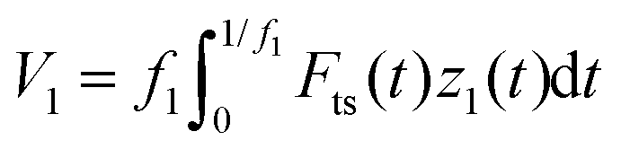
The above equations can be expressed in terms of the observables without knowing the interaction force by integrating the equation of motion (eqn (1)) over a period46,49
V1 = (k1A1A01/2Q1)cos![[thin space (1/6-em)]](https://www.rsc.org/images/entities/char_2009.gif) ϕ1 ϕ1 | (6) |
| V2 = −k2A22Δf2/f02 | (7) |
| Edis1 = πk1A1/Q1(A1 − A01sinϕ1). | (8) |
We note that all the parameters and observables included in eqn (6)–(8) except for ϕ1 and Δf2 are set at the beginning of the experiment. This makes the bimodal AM-FM very efficient because just two data points per pixel are needed to obtain the nanomechanical parameters.
The next step is to solve eqn (3)–(5) in terms of the parameters of a specific tip–surface force Fts. Labuda et al.50 have solved these equations for a force expressed as
 | (9) |
 | (10) |
The above expressions are the general elements of bimodal AFM theory. In what follows we demonstrate that eqn (3)–(5) are solved analytically for a viscoelastic force of the type
| Fts = αδβ + λδμdδ/dt | (11) |
 | (12) |
 | (13) |
 | (14) |
Let's assume that the tip–surface force for a parabolic tip of radius R takes the form of
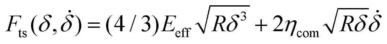 | (15) |
 | (16) |
The combination of Hertz contact mechanics and the mechanical system formed by a spring in parallel with a dash pot is called the 3D Kelvin–Voigt (3D K–V) model (eqn (15)).8,16 We have solved the integrals included in eqn (12)–(14) for the 3D K–V model,
 | (17) |
 | (18) |
 | (19) |
Then, the deformation, the effective Young's modulus and the viscosity coefficient can be expressed as
 | (20) |
 | (21) |
| ηcom = (2πω1)−1EeffEdis1/V1. | (22) |
These expressions enable the bimodal AM-FM to generate images of the true topography of the surface at the same time that it generates maps of the Young's modulus and viscosity coefficient. The step-by-step deduction of the above equations is provided in the ESI.†
The quantity Edis1/V1 coincides with the definition of the loss tangent (tanρ)4,51,52
 | (23) |
2.2 True and apparent topography images
It is known that the force exerted by the tip on a soft matter surface produces a deformation that could affect the determination of its height features.53–56 Thus, an image coming directly from the topographic feedback has to be considered as an image of the apparent topography of the surface (ha). This effect is commonly ignored in AFM because during imaging, the deformation of the sample is entangled with the deflection signal associated with the topography. However, the bimodal AM-FM enables the direct determination of the deformation induced by the force applied by the tip (eqn (20)). Then, the true topography can be obtained by applying the following equation,| htrue(x,y) = ha(x,y) + δmax(x,y). | (24) |
3. Materials and methods
3.1 Polymer samples
The polystyrene (PS) sample (Bruker test sample) with a nominal Young's modulus value of 2.7 GPa is used to calibrate the bimodal AM-FM method (Fig. S1†). The measurements are also performed on a polyolefin elastomer (LDPE sample HarmoniX training sample, Bruker) with an estimated Young's modulus value of around 0.1 GPa.The block copolymer is a poly(styrene-block-methylmethacrylate) (PS-b-PMMA) synthesized as a thin film by self-assembling over a layer of poly(styrene-random-methylmethacrylate) (PS-r-PMMA). The protocol used to make the block copolymer thin film is described elsewhere.57 The block copolymer organizes in a lamellar geometry with a pitch of 30 nm.
3.2 Spatially-resolved viscoelastic maps
The bimodal AFM measurements were performed using a Cypher VRS (Asylum Research Inc.) that enable the control of the temperature and the relative humidity. The experiments were conducted at room temperature (Troom ≈ 25 °C) in a N2 atmosphere. The measurements were done with Asp1 in the 50 to 100 nm range, while A2 was set in the 0.5 to 1.5 nm range. The fast scan rate was 3 Hz.PPP-NCH (Nanosensors) microcantilevers with f01 = 324.783 kHz, k1 = 43.2 N m−1, Q1 = 532, f02 = 2009 kHz, k2 = 2269 N m−1 and f01 = 331.434 kHz, k1 = 54.8 N m−1, Q1 = 596, f02 = 2050 kHz, k2 = 2857 N m−1 have been used to image the LDPE as shown in Fig. 2–4. PPP-FM (Nanosensors) cantilevers with f01 = 77.250 kHz, k1 = 3.2 N m−1, Q1 = 206, f02 = 490.283 kHz, k2 = 166 N m−1 and with f01 = 68.070 kHz, k1 = 2.77 N m−1, Q1 = 208, f02 = 432.333 kHz, k2 = 142 N m−1 have been used to characterize the block copolymer and the polystyrene samples, respectively.
 | ||
| Fig. 2 Apparent, deformation and true topography of a polymer blend. (a) Apparent topography. (b) Deformation. (c) True topography. The bottom panels show the cross-sections across the lines marked in the top panels. The measurement parameters are A01 = 87 nm, A1 = 51 nm, f01 = 324.783 kHz, k1 = 43.2 N m−1, Q1 = 532, A2 = 0.5 nm, f02 = 2009 kHz, k2 = 2269 N m−1, R = 11 nm. | ||
 | ||
| Fig. 3 Nanomechanical maps of a LDPE polymer sample. (a) Young's modulus. (b) Viscosity coefficient. (c) Loss tangent. (d) Retardation time. The bottom panels show the cross-sections obtained across the dashed lines marked in the nanomechanical maps. The blue regions show the values that lie within a 5% window from the average value obtained from the bimodal AM-FM maps. The above images have been obtained with the bimodal AM-FM parameters listed in Fig. 4. A tip radius of 12 nm has been used to fit the data. | ||
 | ||
| Fig. 4 Bimodal AM-FM observables. (a) Set point amplitude of mode 1. The value of Asp1 has been changed 3 nm approximately every 100 nm in the slow scanning direction (vertical axis). (b) Phase shift of the first mode. The map shows the changes due to the change in A1 and reflects the conservative and dissipative contribution of the tip–sample interactions. (c) Frequency shift (Δf2). The variations in Δf2 reflect the elastic response of the LDPE and the changes of the main feedback. (d) Map of the virial of the first mode. The cross-section shows a step-like trend associated with the changes in A1. The measurement parameters are A01 = 54 nm, f01 = 331.434 kHz, k1 = 54.8 N m−1, Q1 = 596, A2 = 0.5 nm, f02 = 2050 kHz, k2 = 2857 N m−1, R = 12 nm. | ||
The force constant of the first mode was calibrated by using the multiple reference calibration method.58 This method avoids the mechanical contact with the sample during the calibration. It is implemented in the software of the Cypher VRS as GetReal™ tool. In the bimodal AM-FM, the calibration of the force constant of the second mode is a critical step.27,57 The second mode of the cantilevers was calibrated by assuming the stiffness–frequency power law relationship, k2 = k1(f2/f1)ζ2, where ζ2 is an experimental calibration parameter.58
Mapping the sample's viscoelastic properties requires the measurements to be performed in the tip–sample repulsive regime.59 To meet this condition ϕ1 must always stay below 90°. During the bimodal AM-FM operation ϕ1 and Δf2 are recorded simultaneously with the tracking of the apparent topography A1 = Asp1. Thus, these observables are used to derive the nanomechanical parameters δ, Eeff, ηcom, tanρ and τ.
The experimental data have been processed by assuming a paraboloid tip. For the LDPE polymer we have assumed radii of 11 nm (PPP-NCH, Fig. 2) and 12 nm (PPP-NCH, Fig. 3 and 4) while for the block copolymer we have assumed R = 2 nm (PPP-FM).
It has been shown that the adsorption of water on a polymer surface could influence the values of some nanomechanical properties, for example, the loss tangent.52 We have confirmed the above observation by measuring the nanomechanical parameters of PS-b-PMMA with and without N2 flow (ESI†). The Young's modulus is not very sensitive to changes in the RH (from 0 to 30%). On the other hand, the viscosity coefficient is increased by increasing the RH. To avoid this effect, the experiments have been performed in a dry N2 atmosphere, with a gas pressure of 0.5 bar.
4. Results and discussion
4.1 Bimodal AM-FM of the polymer (LDPE)
We use LDPE as a test sample to determine the accuracy of the method for measuring the Young's modulus of polymers.10,23 This sample has a nominal Young's modulus of 0.1 GPa. Unfortunately, there is no equivalent test sample to calibrate the viscosity coefficient.Fig. 2a shows the apparent topography of the polymer. The topographic image shows a flat sample with height variations of 1–3 nm. Fig. 2b shows the image of the deformation caused by the tip during the capture of Fig. 2a (Fmax = 30 nN). The deformation is quite uniform across the image, ∼9.5 nm. The near constant value of the deformation across the surface indicates a homogeneous mechanical response. Fig. 2c shows the true topography of the polymer surface after processing the data using eqn (24). We note that the true topography image has a higher spatial resolution than the apparent topography image. This is a bimodal effect due to the dependence of the deformation on the parameters of both models (eqn (20)).
The bimodal AM-FM provides the maps of several properties, such as the Young's modulus, viscosity coefficient, loss tangent or retardation time (Fig. 3). The Young's modulus map (Fig. 3a) shows a homogeneous material characterized by 0.11 ± 0.02 GPa. This value is very close to the nominal value of the LDPE (0.1 GPa). The viscosity coefficient map (Fig. 3b) remains practically constant across the sample (37–40 Pa s). The bimodal AM-FM provides spatially-resolved maps of the retardation times and the loss tangent (Fig. 3c and d). These maps also confirm the nanomechanical homogeneity of the LDPE. To the best of our knowledge Fig. 3d shows the first spatially-resolved map of the retardation times on a polymer. The cross-sections across the polymer are flat (bottom panels). The above parameters have been deduced by assuming a tip radius of 12 nm.
The robustness of the bimodal AM-FM has been tested by studying the dependence of the nanomechanical properties on the operational parameters (A1 in the topography feedback). The images shown in Fig. 3 and 4 have been taken by reducing the set-point amplitude A1 approximately 3 nm in every 100 nm of the slow scanning direction. This gives rise to the stripe-like structure shown in Fig. 4a (top panel) or the staircase shown in the bottom panel. Similar stripes (top panels) or staircases (bottom panels) are observed in other observables such as ϕ1 and Δf2 (Fig. 4b and c), the virial V1 (Fig. 4d) or the energy dissipated (ESI†).
The dependence of the observables, virials and the energy dissipated on the feedback parameters just underlines the fact that these parameters or quantities are not intrinsic properties of the material. However, the nanomechanical parameters of the sample such as the Young's modulus, viscosity coefficient or retardation time are unaffected by these changes (Fig. 3). This result is an indication of the absence of artifacts in the measurements. We underline that the nanomechanical maps shown in Fig. 3 have been obtained by changing the A1 as is indicated in Fig. 4a.
4.2 High spatial resolution viscoelastic maps
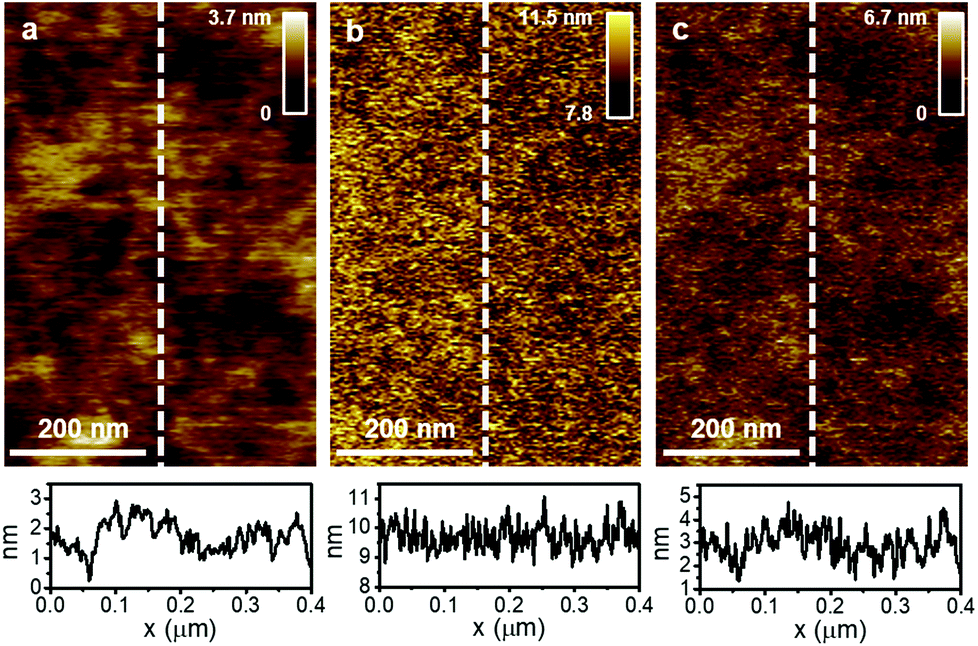
To demonstrate the capabilities of the bimodal AM-FM to generate high spatial resolution maps of viscoelastic properties, we have measured a poly(styrene-block-methylmethacrylate) (PS-b-PMMA) thin film. The diblock copolymer arranges in an ordered lamellar structure alternating PS and PMMA domains with a pitch of 30 nm.13Fig. 5 shows the apparent topography, the deformation and the true topography of the block co-polymer. In the apparent topography image (Fig. 5a), the domains of a component are raised to about 0.3–0.4 nm with respect to the domains of the other component. The Young's modulus map (see below) provides the identification of the domains in terms of the polymer components. The raised features are ascribed to PMMA while the lower features are associated with PS. However, the height difference shown in Fig. 5a does not correspond to the true height difference of the unperturbed polymer surface because the deformation on the PS domains is larger than that on the PMMA domains (EPS < EPMMA). Both PMMA and PS domains are deformed by the force exerted by the tip, respectively, 12.2 nN (PMMA) and 12.9 nN (PS). The deformation measured on PS is of 1.9 nm while that on PMMA is of 1.6 nm (Fig. 5b). Fig. 5c shows the true topography of the block co-polymer.
 | ||
| Fig. 5 Apparent, deformation and true topography of a PS-b-PMMA block co-polymer. (a) Apparent topography. (b) Deformation. (c) True topography. The bottom panels show the cross-sections across the dashed lines marked in the top panels. A01 = 90 nm, A1 = 55 nm, f01 = 77.250 kHz, k1 = 3.2 N m−1, Q1 = 206, A2 = 1.3 nm, f02 = 490.283 kHz, k2 = 166 N m−1, R = 2 nm. | ||
Fig. 6 shows the maps of the viscoelastic parameters acquired simultaneously with the topography. The Young's modulus (Fig. 6a), viscosity coefficient (Fig. 6b) and retardation time (Fig. 6c) maps reproduce the patterns observed in the topography. The alternating PS and PMMA domains generate an oscillation in the values of Young's modulus, viscosity coefficient and retardation time. For the PS domains, Eeff, η and τ are, respectively, 2.1 ± 0.1 GPa, 418 ± 100 Pa s and 0.19 ± 0.04 μs while for the PMMA domains the values are 2.6 ± 0.1 GPa, 186 ± 81 Pa s and 0.08 ± 0.03 μs. In particular, the retardation time shows an oscillatory behavior alternating PS (190 ns) and PMMA (80 ns) domains.
 | ||
| Fig. 6 Nanomechanical maps of a PS-b-PMMA block co-polymer. (a) Young's modulus. (b) Viscosity coefficient. (c) Retardation time. The stiffer domains (PMMA) show a lower viscosity coefficient and a faster response time. The bottom panels show the cross-sections across the lines marked in the top panels. The above images have been obtained simultaneously with those of Fig. 5. A tip radius of 2 nm has been used to deduce the parameters. | ||
4.3 Accuracy of bimodal AM-FM to determine viscoelastic parameters
The accuracy of the bimodal AM-FM to determine viscoelastic parameters can be classified into two different issues. The first issue addresses the validity of the virial and energy balance expressions used in bimodal AFM theory. The second issue addresses the use of the 3D Kelvin–Voigt model and the analytical expressions associated with it to describe the properties of a real polymer sample.The first issue could be considered settled because different numerical simulations and simulators have already validated the use of the approximations involved in the application of the energy balance and virial equations in AFM.60–62
Regarding the second issue, it is well known that the Kelvin–Voigt model does not describe properly the stress relaxation of a viscoelastic material under a fixed strain. In addition, the implementation of the Kelvin–Voigt model for AFM requires an ad hoc assumption about the contact area. We have assumed the contact area changes as in Hertz contact mechanics.16 However, the practical issue is to determine the effect that these limitations have on the quantitative description of the viscoelastic properties of a given polymer sample.
A bimodal AFM experiment implies the application of a time-dependent force that causes a time-dependent deformation. The deformation is dominated by the frequency of the first mode. Thus, a bimodal AFM experiment is very far from a stress relaxation experiment performed at a fixed strain (deformation). In a stress relaxation experiment, the Fourier transform of the deformation has a large number of frequency components. In the linear viscoelastic regime, single frequency deformations are well described by the K–V model. Finite element simulations show that for a paraboloid tip the contact area has a near Hertzian dependence with an indentation during the approaching section of the oscillation.8 In a viscoelastic material, the contact area disagrees with Hertz's theory when the tip is moving away from the sample. The discrepancy between the contact areas increases by increasing the indentation. Thus, the source of error associated with the contact area could be reduced by using relatively small indentations. Fig. 2 and 5 show that the indentation on the softer polymer (LDPE) is 10 nm, on PS is 1.9 nm and on PMMA is 1.6 nm. These deformations could be considered small for a viscoelastic material.
The accuracy of the bimodal AM-FM to determine viscoelastic parameters can be tested by using numerical simulators.60,61 In Fig. 7 we compare the values of the energy dissipated by the tip measured on the LDPE for different amplitude ratios (A1/A01) with the values computed by using the parameters (ELDPE = 0.11 GPa, ηLDPE = 38 Pa s) deduced from bimodal AM-FM theory. The curves show a good agreement between the experimental values and the theory. The relative error in the determination of the energy dissipated with the theory is below 3%. We remark that the experimental determination of the energy dissipated by the tip on the LDPE polymer is exact as long as the oscillation remains sinusoidal. This expression (eqn (5)) does not involve any model of the tip–sample viscoelastic interaction. To illustrate that the agreement is not fortuitous we have plotted the energy dissipated curves obtained by using two different viscosity coefficients, one 10% higher and one 10% lower than the one deduced from the theory. Fig. 7 shows that the experimental values lie between these boundary energy dissipation curves. Another bimodal configuration (FM-FM) has mapped viscoelastic properties of polymers.23 The AM topographic feedback is more stable than FM topographic feedback against changes in the interaction force regime (attractive/repulsive). This makes bimodal AM-FM easier to implement and operate.
 | ||
| Fig. 7 Comparison between numerical simulations and experiments on a LDPE polymer sample. The numerical simulation was performed for a 3D K–V with parameters: Eeff = 111 MPa; ηcom = 38 Pa s. The shaded region shows the values for the dissipated energy if the viscosity coefficient is determined with a 10% relative error. The parameters used for the simulation are listed in Fig. 4. | ||
We are far from claiming that the 3D Kelvin–Voigt model and the analytical expressions derived from it could be applied without any restriction. Our results could be summarized in two main points. First, we provide a self-consistent method to determine the accuracy of any viscoelastic measurement performed by bimodal AFM. This method compares the experimental values of the energy dissipation or the virial with the results obtained with numerical simulations that use the viscoelastic parameters determined by bimodal AFM theory as inputs. Second, we have shown that the 3D Kelvin–Voigt model explains the nanoscale viscoelastic properties of some polymers.
It is hard to compare local and bulk viscoelastic properties because the properties of the polymer region probed by AFM could be affected by surface relaxation processes and interphase interactions. These effects could be negligible in bulk measurements. Some considerations by Raman and co-workers9 and Proksch et al.51 offer additional insights into this issue.
4.4 Tip radius
The tip radius R is a parameter that appears explicitly in the interaction force model (eqn (15)). Its value must be known in order to determine the nanomechanical properties of the sample with the bimodal AM-FM method. Several methods have been proposed to determine the tip radius, ranging from electron microscopy images63 to the in situ characterization by AFM.64 The first approach is time consuming and, more often than not, implies the irreversible damage of the tip, in particular for sharp tips. In situ AFM methods based on studying the transition between attractive and repulsive regimes depend on the ambient conditions. The measurement could also modify the tip radius.Here, we apply a phenomenological approach that involves two complementary estimations of the tip radius. First, the spatial resolution obtained from the nanomechanical map is used to estimate the tip radius (R1 ≈ resolution/2). Second, the effective tip radius has to be larger than the indentation applied in the nanomechanical map (R2 ≥ δ). Then, we choose the maximum of the above values as the tip radius. This value should either be very close or coincide with the value that provides the best fit with the experimental data.
5. Conclusions
Bimodal AFM has expanded the characterization of surfaces at the nanoscale by providing high resolution maps of several viscoelastic parameters. The bimodal AM-FM configuration enables the simultaneous acquisition of the topography, the elastic modulus, the viscosity coefficient, the retardation time and the loss tangent of a sample without introducing additional limitations on the imaging acquisition rate. We have developed the theory of bimodal AM-FM to transform the observables into the viscoelastic parameters in terms of the 3D Kelvin–Voigt model. This theory enables the mapping of the Young's modulus, viscosity coefficient and retardation time at the same time that the true topography of the material is acquired. The accuracy and spatial resolution has been tested on a homogeneous polymer and a block copolymer sample. We have shown that the nanomechanical measurements are very robust with respect to the choice of the feedback parameters. We have also provided the first theoretical demonstration of the relationship between the loss tangent and an intrinsic viscoelastic parameter of the sample.The bimodal AM-FM has several key features that are not found in other AFM-based mapping methods. First, it is very efficient. It just requires the recording of two data points per pixel to generate four different nanomechanical maps. Second, it measures the deformation generated during imaging in real time, thus providing the true topography of the sample. Third, it is fast. The generation of multiple nanoscale maps does not compromise the imaging speed.
Measuring the viscoelastic properties at the nanoscale poses several challenging issues that range from the choice of the linear viscoelastic model to the fact that viscoelasticity is a frequency-dependent process. We provide a criterion to determine whether the model and/or the measured viscoelastic parameters provide a faithful characterization of the sample. In summary, this contribution completes the characterization capabilities of bimodal force microscopy by providing a fast, robust, reliable and high resolution method to measure the local viscoelastic properties of soft matter.
Conflicts of interest
The authors declare no competing interest.Acknowledgements
We thank the financial support from the European Research Council ERC–AdG–340177 (3DNanoMech) and the Ministerio de Economía y Competitividad for grants CSD2010-00024 and MAT2016-76507-R. This work has received funding from the European Union's Horizon 2020 research and innovation programme under the Marie Sklodowska-Curie grant agreement No. 721874 (SPM2.0). The fellowship FPU15/04622 from the Ministerio de Educación is also acknowledged.Notes and references
- M. Chyasnavichyus, S. L. Young and V. V. Tsukruk, Langmuir, 2014, 30, 10566–10582 CrossRef CAS PubMed.
- S. D. Solares, Beilstein J. Nanotechnol., 2014, 5, 1649–1663 CrossRef PubMed.
- H. K. Nguyen, M. Ito and K. Nakajima, Jpn. J. Appl. Phys., 2016, 55, 08NB06 CrossRef.
- R. Proksch, M. Kocun, D. C. Hurley, M. Viani, A. Labuda, W. Meinhold and J. Bemis, J. Appl. Phys., 2016, 119, 134901 CrossRef.
- J. S. de Sousa, J. A. C. Santos, E. B. Barros, L. M. R. Alencar, W. T. Cruz, M. V. Ramos and J. Mendes Filho, J. Appl. Phys., 2017, 121, 034901 CrossRef.
- Y. M. Efremov, W.-H. Wang, S. D. Hardy, R. L. Geahlen and A. Raman, Sci. Rep., 2017, 7, 1541 CrossRef PubMed.
- M. R. Uhlig and R. Magerle, Nanoscale, 2017, 9, 1244–1256 RSC.
- P. D. Garcia and R. Garcia, Biophys. J., 2018, 114, 2923–2932 CrossRef CAS PubMed.
- B. Rajabifar, J. M. Jadhav, D. Kiracofe, G. F. Meyers and A. Raman, Macromolecules, 2018, 51, 9649–9661 CrossRef CAS.
- F. Crippa, P. A. Thorén, D. Forchheimer, R. Borgani, B. Rothen-Rutishauser, A. Petri-Fink and D. Haviland, Soft Matter, 2018, 14, 3998–4006 RSC.
- D. Wang and T. P. Russell, Macromolecules, 2018, 51, 3–24 CrossRef CAS.
- R. Garcia, A. W. Knoll and E. Riedo, Nat. Nanotechnol., 2014, 9, 577–587 CrossRef CAS PubMed.
- S. Gottlieb, M. Lorenzoni, L. Evangelio, M. Fernández-Regúlez, Y. K. Ryu, C. Rawlings, M. Spieser, A. W. Knoll and F. Perez-Murano, Nanotechnology, 2017, 28, 175301 CrossRef CAS PubMed.
- E. Moeendarbary, L. Valon, M. Fritzsche, A. R. Harris, D. A. Moulding, A. J. Thrasher, E. Stride, L. Mahadevan and G. T. Charras, Nat. Mater., 2013, 12, 253–261 CrossRef CAS PubMed.
- J. Rother, H. Noding, I. Mey and A. Janshoff, Open Biol., 2014, 4, 140046–140046 CrossRef PubMed.
- P. D. Garcia, C. R. Guerrero and R. Garcia, Nanoscale, 2017, 9, 12051–12059 RSC.
- A. Rigato, A. Miyagi, S. Scheuring and F. Rico, Nat. Phys., 2017, 13, 771–775 Search PubMed.
- P. Attard, J. Phys.: Condens. Matter, 2007, 19, 473201 CrossRef.
- R. Garcia, C. J. Gómez, N. F. Martinez, S. Patil, C. Dietz and R. Magerle, Phys. Rev. Lett., 2006, 97, 1–4 Search PubMed.
- E. A. López-Guerra, F. Banfi, S. D. Solares and G. Ferrini, Sci. Rep., 2018, 8, 7534 CrossRef PubMed.
- S. D. Solares, Beilstein J. Nanotechnol., 2016, 7, 554–571 CrossRef CAS PubMed.
- T. R. Rodríguez and R. Garcia, Appl. Phys. Lett., 2004, 84, 449–451 CrossRef.
- E. T. Herruzo, A. P. Perrino and R. Garcia, Nat. Commun., 2014, 5, 3126 CrossRef PubMed.
- D. Martinez-Martin, E. T. Herruzo, C. Dietz, J. Gomez-Herrero and R. Garcia, Phys. Rev. Lett., 2011, 106, 1–4 CrossRef PubMed.
- G. Lamour, C. K. Yip, H. Li and J. Gsponer, ACS Nano, 2014, 8, 3851–3861 CrossRef CAS PubMed.
- C. A. Amo, A. P. Perrino, A. F. Payam and R. Garcia, ACS Nano, 2017, 11, 8650–8659 CrossRef CAS PubMed.
- S. Benaglia, V. G. Gisbert, A. P. Perrino, C. A. Amo and R. Garcia, Nat. Protoc., 2018, 13, 2890–2907 CrossRef CAS PubMed.
- M. Kocun, A. Labuda, W. Meinhold, I. Revenko and R. Proksch, ACS Nano, 2017, 11, 10097–10105 CrossRef CAS PubMed.
- C. Y. Lai, S. Santos and M. Chiesa, ACS Nano, 2016, 10, 6265–6272 CrossRef CAS PubMed.
- A. X. Cartagena-Rivera, W.-H. Wang, R. L. Geahlen and A. Raman, Sci. Rep., 2015, 5, 11692 CrossRef CAS PubMed.
- D. Guan, E. Charlaix, R. Z. Qi and P. Tong, Phys. Rev. Appl., 2017, 8, 1–6 Search PubMed.
- Y. Sun, L. H. Vu, N. Chew, Z. Puthucheary, M. E. Cove and K. Zeng, ACS Biomater. Sci. Eng., 2019, 5, 478–486 CrossRef CAS.
- Z. Al-Rekabi and S. Contera, Proc. Natl. Acad. Sci. U. S. A., 2018, 115, 2658–2663 CrossRef CAS PubMed.
- W. Trewby, J. Faraudo and K. Voïtchovsky, Nanoscale, 2019, 11, 4376–4384 RSC.
- E.-N. Athanasopoulou, N. Nianias, Q. K. Ong and F. Stellacci, Nanoscale, 2018, 10, 23027–23036 RSC.
- C. Albonetti, S. Casalini, F. Borgatti, L. Floreano and F. Biscarini, Chem. Commun., 2011, 47, 8823–8825 RSC.
- Y. Li, C. Yu, Y. Gan, P. Jiang, J. Yu, Y. Ou, D.-F. Zou, C. Huang, J. Wang, T. Jia, Q. Luo, X.-F. Yu, H. Zhao, C.-F. Gao and J. Li, npj Comput. Mater., 2018, 4, 49 CrossRef.
- R. Giridharagopal, L. Q. Flagg, J. S. Harrison, M. E. Ziffer, J. Onorato, C. K. Luscombe and D. S. Ginger, Nat. Mater., 2017, 16, 1–6 CrossRef PubMed.
- R. Garcia and R. Proksch, Eur. Polym. J., 2013, 49, 1897–1906 CrossRef CAS.
- R. Garcia and E. T. Herruzo, Nat. Nanotechnol., 2012, 7, 217–226 CrossRef CAS PubMed.
- D. Ebeling and S. D. Solares, Beilstein J. Nanotechnol., 2013, 4, 198–207 CrossRef PubMed.
- S. Kawai, T. Glatzel, S. Koch, B. Such, A. Baratoff and E. Meyer, Phys. Rev. B: Condens. Matter Mater. Phys., 2010, 81, 085420 CrossRef.
- C. Dietz, Nanoscale, 2018, 10, 460–468 RSC.
- J. R. Lozano and R. Garcia, Phys. Rev. Lett., 2008, 100, 8–11 CrossRef PubMed.
- A. San Paulo and R. Garcia, Phys. Rev. B: Condens. Matter Mater. Phys., 2001, 64, 193411 CrossRef.
- E. T. Herruzo and R. Garcia, Beilstein J. Nanotechnol., 2012, 3, 198–206 CrossRef PubMed.
- S. Kawai, T. Glatzel, S. Koch, B. Such, A. Baratoff and E. Meyer, Phys. Rev. Lett., 2009, 103, 220801 CrossRef PubMed.
- M. D. Aksoy and A. Atalar, Phys. Rev. B: Condens. Matter Mater. Phys., 2011, 83, 075416 CrossRef.
- J. R. Lozano and R. Garcia, Phys. Rev. B: Condens. Matter Mater. Phys., 2009, 79, 014110 CrossRef.
- A. Labuda, M. Kocun, W. Meinhold, D. Walters and R. Proksch, Beilstein J. Nanotechnol., 2016, 7, 970–982 CrossRef CAS PubMed.
- R. Proksch and D. G. Yablon, Appl. Phys. Lett., 2012, 100, 073106 CrossRef.
- H. K. Nguyen, X. Liang, M. Ito and K. Nakajima, Macromolecules, 2018, 51, 6085–6091 CrossRef CAS.
- A. San Paulo and R. Garcia, Biophys. J., 2000, 78, 1599–1605 CrossRef CAS.
- A. Knoll, R. Magerle and G. Krausch, Macromolecules, 2001, 34, 4159–4165 CrossRef CAS.
- D. Wang, S. Fujinami, K. Nakajima and T. Nishi, Macromolecules, 2010, 43, 3169–3172 CrossRef CAS.
- A. P. Perrino and R. Garcia, Nanoscale, 2016, 8, 9151–9158 RSC.
- S. Gottlieb, D. Kazazis, I. Mochi, L. Evangelio, M. Fernández-Regúlez, Y. Ekinci and F. Perez-Murano, Soft Matter, 2018, 14, 6799–6808 RSC.
- A. Labuda, M. Kocun, M. Lysy, T. Walsh, J. Meinhold, T. Proksch, W. Meinhold, C. Anderson and R. Proksch, Rev. Sci. Instrum., 2016, 87, 073705 CrossRef PubMed.
- R. Garcia and A. San Paulo, Phys. Rev. B: Condens. Matter Mater. Phys., 1999, 60, 4961–4967 CrossRef CAS.
- J. Melcher, S. Hu and A. Raman, Rev. Sci. Instrum., 2008, 79, 061301 CrossRef PubMed.
- H. V. Guzman, P. D. Garcia and R. Garcia, Beilstein J. Nanotechnol., 2015, 6, 369–379 CrossRef CAS PubMed.
- S. An, S. D. Solares, S. Santos and D. Ebeling, Nanotechnology, 2014, 25, 475701 CrossRef PubMed.
- V. Vahdat and R. W. Carpick, ACS Nano, 2013, 7, 9836–9850 CrossRef CAS PubMed.
- S. Santos, L. Guang, T. Souier, K. Gadelrab, M. Chiesa and N. H. Thomson, Rev. Sci. Instrum., 2012, 83, 043707 CrossRef PubMed.
Footnote |
| † Electronic supplementary information (ESI) available. See DOI: 10.1039/c9nr04396a |
| This journal is © The Royal Society of Chemistry 2019 |