
 Open Access Article
 This Open Access Article is licensed under a
 Creative Commons Attribution 3.0 Unported Licence
Total generalized variation regularization for multi-modal electron tomography†
Richard
Huber
 *a,
Georg
Haberfehlner
*bc,
Martin
Holler
*ad,
Gerald
Kothleitner
*bc and
Kristian
Bredies
*a
*a,
Georg
Haberfehlner
*bc,
Martin
Holler
*ad,
Gerald
Kothleitner
*bc and
Kristian
Bredies
*a
aInstitute for Mathematics and Scientific Computing, University of Graz, Heinrichstraße 36, A-8010 Graz, Austria. E-mail: richard.huber@uni-graz.at; martin.holler@uni-graz.at; kristian.bredies@uni-graz.at
bInstitute of Electron Microscopy and Nanoanalysis, Graz University of Technology, Steyrergasse 17, 8010 Graz, Austria. E-mail: georg.haberfehlner@felmi-zfe.at; gerald.kothleitner@felmi-zfe.at
cGraz Centre for Electron Microscopy, Steyrergasse 17, 8010 Graz, Austria
dCentre de Mathématiques Appliquées, École Polytechnique, 91128 Palaiseau Cedex, France
First published on 28th February 2019
Abstract
In multi-modal electron tomography, tilt series of several signals such as X-ray spectra, electron energy-loss spectra, annular dark-field, or bright-field data are acquired at the same time in a transmission electron microscope and subsequently reconstructed in three dimensions. However, the acquired data are often incomplete and suffer from noise, and generally each signal is reconstructed independently of all other signals, not taking advantage of correlation between different datasets. This severely limits both the resolution and validity of the reconstructed images. In this paper, we show how image quality in multi-modal electron tomography can be greatly improved by employing variational modeling and multi-channel regularization techniques. To achieve this aim, we employ a coupled Total Generalized Variation (TGV) regularization that exploits correlation between different channels. In contrast to other regularization methods, coupled TGV regularization allows to reconstruct both hard transitions and gradual changes inside each sample, and links different channels at the level of first and higher order derivatives. This favors similar interface positions for all reconstructions, thereby improving the image quality for all data, in particular, for 3D elemental maps. We demonstrate the joint multi-channel TGV reconstruction on tomographic energy-dispersive X-ray spectroscopy (EDXS) and high-angle annular dark field (HAADF) data, but the reconstruction method is generally applicable to all types of signals used in electron tomography, as well as all other types of projection-based tomographies.
Introduction
Electron tomography using a scanning transmission electron microscope (STEM) is a versatile tool for the investigation of nanomaterials in three dimensions down to the single atomic level.1,2 Insight into the 3D elemental and chemical make-up of a sample is provided by the spectroscopic signals originating from inelastic scattering in analytical tomography experiments.3 Energy losses of electrons traversing a thin TEM specimen can be measured using energy-filtered TEM (EFTEM)4–7 or electron energy-loss spectroscopy (EELS)8–10 and characteristic X-rays can be recorded using energy-dispersive X-ray spectroscopy (EDXS).11–13 Also, EELS and EDXS signals can be acquired simultaneously for combined analytical tomography experiments.14 Over the last few years, analytical tomography has thereby become an important characterization method in nanoscale materials science.13,15–18The 3D resolution of a sinogram is generally limited by the number of projections which can be acquired in an experiment and by the achievable tilt range. Reasons for these limitations are the overall dose the sample can sustain, the accuracy of the sample positioning mechanism for very small tilt steps, the geometry of the sample or the sample holder, as well as the limited time for an experiment. This leads to the situation that image reconstruction from an electron tomography experiment usually amounts to solving an ill-posed inverse problem with more unknown parameters than measurements. Especially for analytical tomography data, also the signal-to-noise ratio is very low. Therefore, a priori knowledge and regularization are essential to find better solutions for a tomographic reconstruction. In this context sparse recovery has become increasingly important over the last few years.19–22 In sparse recovery, the signal of interest is assumed to have sparse representation when transformed to a suitable basis. If such a transformation is possible, minimization of the ![[small script l]](https://www.rsc.org/images/entities/char_e146.gif) 1-norm in this domain enforces sparsity and can lead to an accurate solution.
1-norm in this domain enforces sparsity and can lead to an accurate solution.
The most important type of sparsity in electron tomography is sparsity of the image (or volume) gradient.19,23,24 Known as Total Variation (TV)25 minimization, 1-minimization of the image gradient leads to an image (or volume) with locally constant regions, separated by sharp interfaces. For materials science samples, it can often be assumed that well separated phases exist within a sample, which is why TV minimization has found a range of applications in electron tomography.26–29 It has been shown that TV minimization can be especially favorable for analytical electron tomography experiments, where usually only limited and noisy data are available.14,30
Two major limitations can be identified with current TV minimization approaches and their application in analytical tomography. First, the underlying model of TV minimization assumes that the sample only contains sharp interfaces between different phases, severely restricting the range of materials that can be analyzed using TV minimization. All types of gradual changes between different sample regions, such as diffusion at interfaces, are typically not correctly recovered. Second, in analytical tomography and other multi-modal tomography experiments, different signals are acquired at the same time, containing complementary information. But in most approaches this is not exploited but rather each signal is reconstructed independently. Until recently, there was only one attempt to link the information of different signals,31 where the intensity of the HAADF signal was expressed as a linear combination of EDXS signals and reconstructed with a conventional reconstruction algorithm.
Here we present an approach for resolving these issues for multi-modal tomography. We apply coupled Total Generalized Variation (TGV)32–34 regularization, which allows for both sharp interfaces and gradual intensity changes in the reconstruction and exploits inter-channel correlation. This yields a joint multi-channel reconstruction of HAADF and EDXS data. We demonstrate our approach on phantom data and on an Al-5 wt% Si alloy with 50 ppm Na and 6100 ppm Yb,14 where the precipitation of Yb and Si takes place at the nanoscale, but it is generally applicable to analytical electron tomography of all types of nanostructured materials. The basic concept of multi-modal STEM tomography is depicted in Fig. 1. Several tilt series are acquired at the same time in the microscope. In the joint reconstruction all tilt series are used together to obtain a joint multi-modal reconstruction.
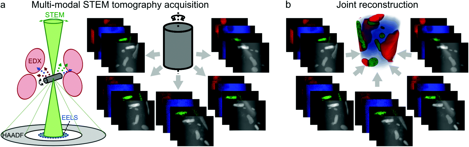 | ||
| Fig. 1 Basic principles of multi-modal STEM tomography. (a) Simultaneous acquisition of several tilt series (EDXS/EELS+HAADF). (b) Joint reconstruction of all tilt series. | ||
We note that in two recent, independent studies,35,36 a coupled Total Variation approach was proposed to link data and create smooth reconstructions. While these studies overcome the second limitation of existing approaches as mentioned above, the usage of TV regularization still limits their applicability to piecewise constant densities with sharp interfaces. However, a major benefit of three-dimensional local elemental distributions lies in analyzing local concentration variations. While the compositions of well separated phases are often accessible already by 2D investigations after appropriate sample preparation, local variations are always masked due to projection. A recent example is the unveiling of elemental concentration variations within spherical precipitates in an AlMgScZr-alloy.17 In such situations it would not be possible to use TV regularization. Beyond overcoming this drawback, a second novelty of our approach is that we developed – and make publicly available37 – a Python38/OpenCL39-based implementation for all components of the reconstruction algorithm, which is crucial in particular for 3D reconstructions as it significantly reduces the computation time. A graphical user interface connected to the code allows for simple and efficient execution. In particular, we developed a custom, GPU-based implementation of the forward operator and its adjoint, ensuring, in contrast to other existing implementations, numerical adjointness of the two, which is in particular crucial for the convergence of iterative minimization algorithms.
We also note that TGV regularization for both single- and multi-channel data has been demonstrated to work well and to be superior to TV regularization in various applications.40–45 In particular, in the context of joint magnetic resonance (MR) imaging and positron emission tomography (PET), multi-channel TGV regularization was shown to allow for improved recovery of quantitative measurements compared to single-channel approaches.46 Also theoretical results on well-posedness and stability for multi-channel regularization are available.47 Building on the existing code for MR reconstruction,40 a first application of TGV in the context of two-dimensional single-channel electron tomography was also presented in a conference proceedings paper48 and shown to be superior to TV regularization.
Results
The main principles of multi-modal TGV reconstruction
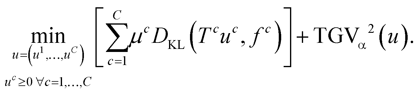
The proposed tomographic reconstruction framework is based on a convex variational method employing volumetric coupled second order Total Generalized Variation (TGV) regularization, and the Kullback–Leibler (KL) divergence as a discrepancy measure. Given some measured multi-channel‡ data f = (f![[thin space (1/6-em)]](https://www.rsc.org/images/entities/char_2009.gif) 1, …, fC), a reconstruction u = (u1, …, uC) is obtained as a solution to the convex minimization problem
1, …, fC), a reconstruction u = (u1, …, uC) is obtained as a solution to the convex minimization problem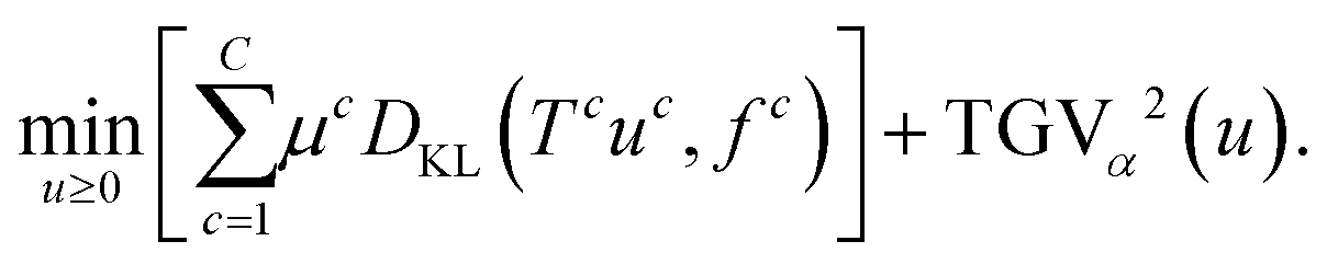 | (1) |
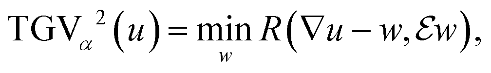
Here, 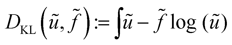 corresponds (up to constants and non-negativity constraints) to the Kullback–Leibler divergence, which is an appropriate data fidelity measure in the presence of Poisson noise. The operators Tc map each image channel to the corresponding data space and comprise a slice-wise Radon transform and a possible change of resolution. For the sake of simplicity we assume that for c = 1, …, C the forward operators are identical, i.e. Tc = T, although the theory is not limited to such restrictions. The regularization parameters μc ensure the trade-off between data fidelity and regularization for each channel. The functional TGVα2 is given as
 | (2) |
 denotes a symmetrized Jacobian of w. The norms |·|frob are pointwise Frobenius matrix and tensor norms and ‖·‖1 denotes the one-norm, i.e., the sum of moduli over all image voxels. For solving the minimization problem (1), we employ a duality-based algorithm for which we developed a Python38/OpenCL39 implementation. Further details of the algorithm and the reconstruction approach are provided in the section Materials and methods.
We can identify two main features of the proposed coupled TGV regularization functional: first, the functional itself optimally balances between a penalization of the first and second order derivatives. Choosing the auxiliary variable w to be locally zero or equal to ∇u, it is possible to penalize either the one-norm of ∇u or the one-norm of  , where
  corresponds to the Hessian of u. For this reason the proposed method can be expected to recover both sharp interfaces and gradual intensity changes. Second, the pointwise matrices and tensors resulting from differentiation of u and w are coupled with a Frobenius norm, i.e., the two-norm over all entries. This enforces joint sparsity of the corresponding quantities; in particular, the edge set of each channel can be expected to have small support and to largely coincide with the ones of the other channels.
Reconstruction of phantom data
To illustrate the capability of the joint TGV algorithm, we first test it in an artificial example. For this purpose we created a multi-channel phantom object. The phantom is inspired by the sample investigated in our experiments and is assumed to consist of three elements (Yb, Si and Al), with both abrupt and gradual concentration changes in the sample. For this phantom, we calculate the sinograms of EDX signals for Yb, Si and Al and of the HAADF signal assuming typical experimental parameters for an analytical tomography experiment and add Poisson noise to the calculated sinograms (see the Materials and methods section). To investigate how a full 3D implementation of the reconstruction algorithm compares to a 2D implementation, we replicate the same slice 60 times rotating each slice slightly compared to the previous to obtain a 3D volume with changes along all three dimensions. Fig. 2 shows the phantom and the sinograms with and without noise. For each slice, sinograms are calculated with a size of 305 pixels over a range of 180° with steps of 5° (see the Materials and methods section for more details of the phantom). | ||
| Fig. 2 Multi-channel 3D phantom: (a) HAADF slices along three orthogonal directions, (b) HAADF sinogram without noise and (c) with noise (peak signal-to-noise ratio (PSNR): 55 dB). (d) EDX slices, (e) EDX sinograms without noise and (f) with noise (PSNR for Yb: 7.77 dB, for Si: 9.25 dB, for Al: 18.21 dB). Yb is shown in green, Si in red and Al in blue. | ||
For reconstruction, we compare the standard method SIRT49 with TV and TGV regularization, where for the latter two we provide the results for 2D slice-wise and volumetric 3D regularization as well as uncoupled and coupled regularization of the different channels. The SIRT reconstructions were obtained using the Astra toolbox50,51 and for the TV and TGV results, we used different variants of our reconstruction algorithm presented in the Materials and methods section. Reconstruction parameters for all methods are provided in ESI Table 1.†
In Fig. 3 we provide the reconstruction results, where three orthogonal slices for each method for both the HAADF and the EDXS signals are compared to the original phantom (Fig. 3a). The SIRT reconstruction (Fig. 3b) of the low-noise HAADF data is quite acceptable, showing only some typical artifacts stemming from the limited number of projections. Due to the low signal of the EDXS data however, these reconstructions are dominated by the Poisson noise of the sinograms and hardly anything can be discerned.
 | ||
| Fig. 3 Reconstructions of a phantom from noisy projection data. In the images, Al is depicted in blue, Si in red and Yb in green. (a) Original phantom, (b) SIRT reconstruction, (c) 2D TV reconstruction without coupling, (d) 2D TGV2 reconstruction without coupling, (e) 2D coupled TV reconstruction, (f) 2D coupled TGV2 reconstruction, (g) 3D TV reconstruction without coupling, (h) 3D TGV2 reconstruction without coupling, (i) 3D coupled TV reconstruction, and (j) 3D coupled TGV2 reconstruction. | ||
Introducing variational regularization reduces the impact of noise on the reconstruction, but it can be observed that the results strongly depend on the chosen regularizer. In an uncoupled 2D TV reconstruction (Fig. 3c) severe staircasing artifacts (i.e., artificial piecewise constant regions) are present; these artifacts are removed by using the TGV2 norm (Fig. 3d), but in both these reconstructions small features in the sample can completely disappear due to the low signal-to-noise ratio of the sinograms.
This situation can be significantly improved by coupling the reconstructions for both TV (Fig. 3e) and TGV2 (Fig. 3f). With the transfer of information between the channels the presence and shape of smaller features become clear also in the reconstructions of EDXS data. In the TGV2 reconstruction, both sharp and gradual concentration changes can be recovered and also in the TV reconstruction, staircasing artifacts are reduced.
By linking all slices in the third spatial dimension, the 3D implementation of the algorithm is even more robust to noise for both the uncoupled (Fig. 3g & h) and the joint reconstruction (Fig. 3i & j). The 3D joint reconstruction methods make full use of data correlation, along all three spatial dimensions as well as between the different channels and therefore give the best reconstruction for both TV and TGV2. With TGV2, constant areas and hard transitions are equally well reconstructed as with TV, but, by promoting piecewise linear functions in addition to sharp interfaces, TGV2 is superior to TV when it comes to gradual intensity changes. In the TGV2 reconstruction all but some of the very smallest features can be recovered.
These trends in improvement can also be quantified by considering the corresponding peak signal-to-noise ratios between the original phantom images and the reconstructions, as shown in Table 1. We see, for example, that the PSNR of the ytterbium reconstructions strongly benefits from the coupling of channels both in 2D and 3D. Also, all channels greatly benefit from the change from 2D to 3D. Note that, even though visually one can observe qualitative improvements with TGV compared to TV, both methods behave similarly in terms of PSNR. This may be explained using the fact that PSNR is not well suited to quantify such qualitative differences, but also by the fact that the parameters for the reconstruction of Fig. 3 were selected for visually optimal results. Indeed, reducing the amount of regularization slightly can be expected to yield an improvement in terms of PSNR for all methods, but would decrease the visual image quality. Nevertheless, we see that also in terms of PSNR, the improvement obtained with the proposed coupled 3D TGV reconstruction is quite significant compared to 2D uncoupled reconstructions or the SIRT method. In this context, we also refer the reader to the ESI† of this paper, where a mean-to-standard-deviation evaluation of our method on 100 different noise realizations also revealed that a significant improvement was obtained with TGV both for the mean over all reconstructions from different noise realizations and for the standard deviation.
| SIRT | TV uncorr. 2D | TV coupled 2D | TV uncorr. 3D | TV coupled 3D | |
|---|---|---|---|---|---|
| HAADF | 19.05 | 34.56 | 34.59 | 35.15 | 35.05 |
| Ytterbium | 2.72 | 6.22 | 10.14 | 10.71 | 13.42 |
| Aluminum | 8.26 | 14.83 | 15.80 | 18.42 | 18.78 |
| Silicon | 3.19 | 9.17 | 9.94 | 12.09 | 13.18 |
| TGV uncorr. 2D | TGV coupled 2D | TGV uncorr. 3D | TGV coupled 3D | |
|---|---|---|---|---|
| HAADF | 35.10 | 35.06 | 35.21 | 35.23 |
| Ytterbium | 7.92 | 10.74 | 11.40 | 14.09 |
| Aluminum | 14.66 | 15.25 | 18.03 | 18.28 |
| Silicon | 9.13 | 9.85 | 10.98 | 12.44 |
Experimental reconstruction
In an analytical tomography experiment we acquired tilt series from a needle-shaped sample prepared from an Al-5 wt% Si alloy with 50 ppm Na and 6100 ppm Yb. HAADF STEM data and EDXS spectrum images were acquired every 4° with a pixel size of 0.76 nm. HAADF data and elemental maps of Yb, Si and Al at different tilt angles are shown in Fig. 4. | ||
| Fig. 4 (a) HAADF STEM projections and (b) sinograms of the HAADF STEM signal at three different heights as indicated by dashed lines in (a). (c) Projections of Yb, Si and Al EDXS signals at different tilt angles and (d) sinograms of the Yb, Si and Al EDXS signals at three different heights as indicated by dashed lines in (c). The individual signals of Yb, Si and Al are shown in the ESI Fig. 2.† | ||
Reconstructions of the HAADF and EDXS data using the SIRT method as well as uncoupled and coupled TGV regularization are shown in Fig. 5, where for the SIRT method we used 100 and 20 iterations for the HAADF and EDXS data, respectively, and we refer the reader to the section Materials and methods for the parameter choice for TGV. Fig. 5a depicts a conventional SIRT reconstruction and Fig. 5b an uncoupled TGV2 reconstruction. For both the HAADF and the EDXS data the quality improvements of TGV reconstruction are evident. In the HAADF reconstruction of the shown slice, two bright features are visible, and in the larger one, dark enclosures are present. These are already visible in the SIRT reconstruction, but are much clearer in the TGV2 reconstruction. Furthermore, in the TGV2 reconstruction, it becomes evident that at the interfaces of the bright features, both abrupt and gradual transitions are present at different locations. For the reconstructions of the EDXS data, TGV2 significantly reduces the impact of noise on the reconstruction, but smaller features, such as the dark enclosures of the HAADF image, are not visible in the EDXS data neither in the SIRT reconstruction nor in the uncoupled TGV2 reconstruction. As Yb is by far the heaviest element present in the sample, HAADF contrast is governed by the local Yb concentration, and therefore at the locations of the enclosures, the EDXS signal of Yb should decrease.
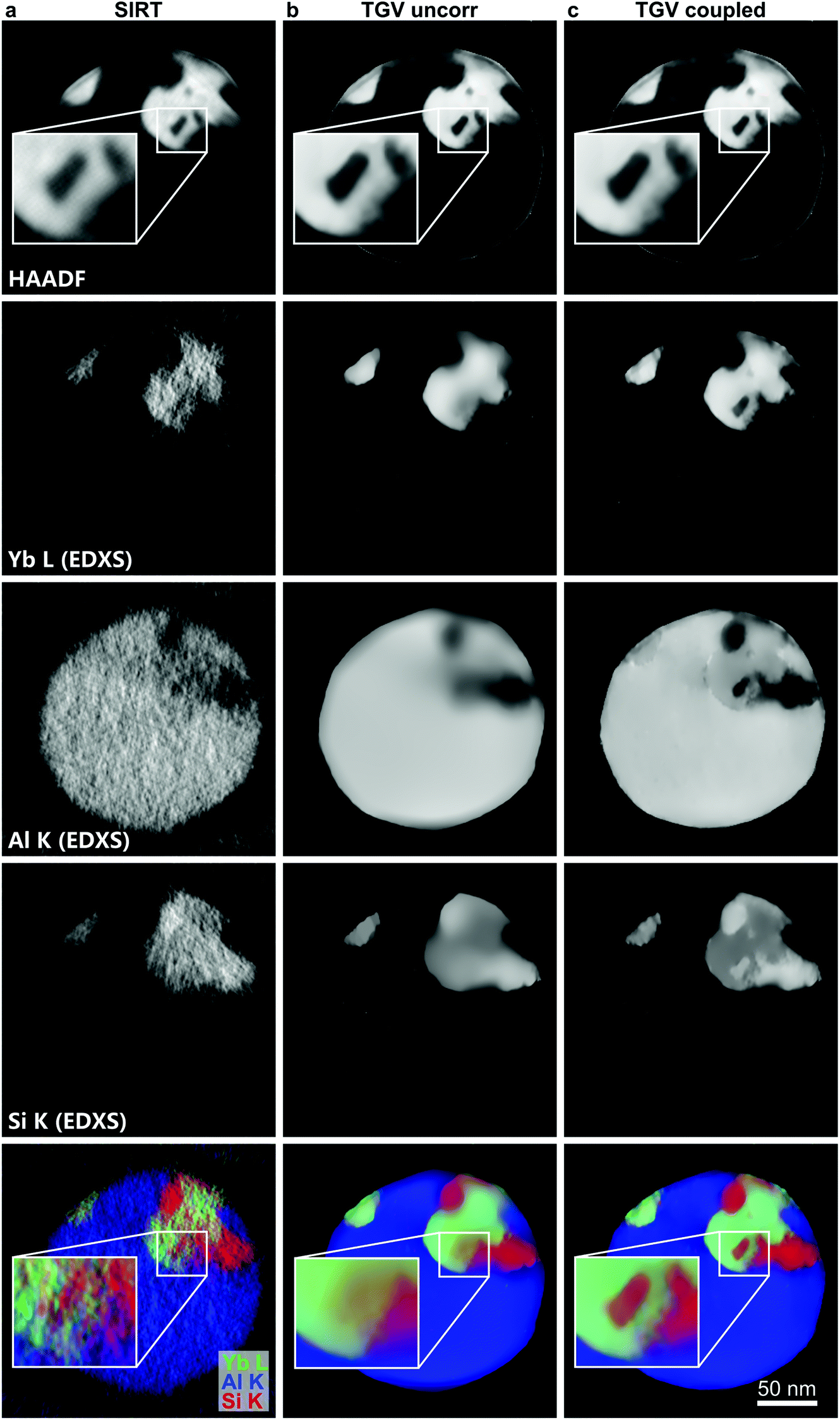 | ||
| Fig. 5 Reconstruction of HAADF data and Yb, Si and Al elemental maps. (a) Uncorrelated SIRT reconstruction, (b) uncorrelated TGV reconstruction, and (c) joint TGV reconstruction. | ||
This issue can be resolved in the joint TGV2 reconstruction depicted in Fig. 5c. Due to the coupling, the reconstructions of the elemental maps show much better defined interfaces and transitions. It is now evident that the dark enclosures visible in the HAADF image correspond to areas with a low concentration of Yb and a high concentration of Si. This is a result of the coupling of the signals, as the transition locations present in the HAADF signals are transferred to the reconstructed elemental maps. In the coupled reconstruction it can also be observed that gradual transitions between different areas are present at some of the interfaces between Yb-rich and Si-rich regions and near the edge of the sample, where beam damage during sample preparation plays a role. In contrast, all interfaces between Yb-rich regions and the Al-matrix are abrupt.
It should be noted that for both the TV and TGV2 reconstruction, regularization parameters have been chosen to weight the impact of the norms. A comparison of the effect of different regularization parameters for experimental data is given in Fig. 6. In Fig. 6a the regularization parameter for the HAADF data is varied, while in Fig. 6b the parameter for the HAADF data is kept constant, and the parameters for the EDXS data are changed by the same factor. By visual comparison of different parameters, good parameters can be chosen, which do not lead to a loss of information, while minimizing the impact of noise on the reconstruction. In the section Materials and methods we expand in more detail on how to choose these parameters. Note that also for SIRT and similar methods, a parameter (typically the number of iterations) must be chosen for each channel. The impact of SIRT parameters is depicted in ESI Fig. 3.† In this context, and in contrast to SIRT, one should also note that the number of iterations for our method does not play the role of an additional parameter but rather just needs to be chosen sufficiently high such that convergence is ensured.
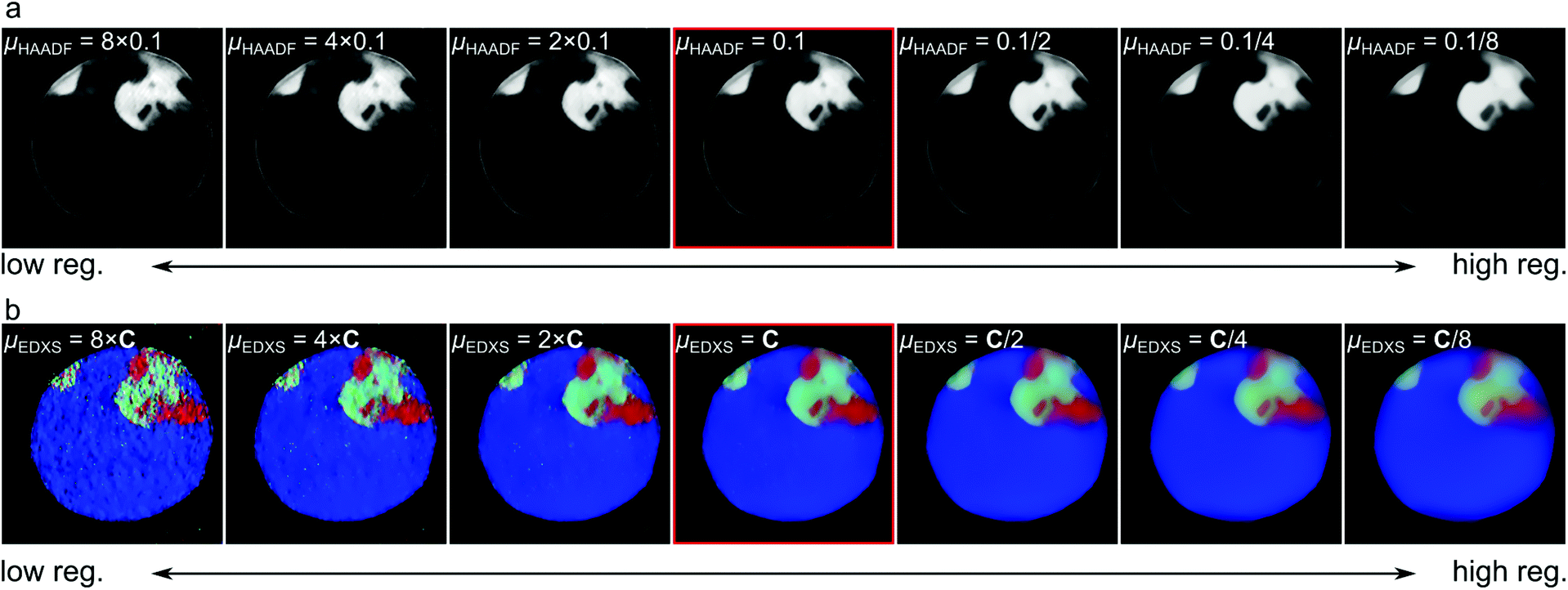 | ||
| Fig. 6 Comparison of different regularization parameters for TGV reconstructions of the experimental data: (a) for the HAADF data and (b) for the EDXS data. In (b), μHAADF = 0.1 for all reconstructions and for the central image C = (μAl, μSi, μYb) = (0.0024, 0.0014, 0.001). | ||
Fig. 7 shows several slices through the linked reconstruction of all signals and a volume rendering of the different signals. As the HAADF signal is governed by the local Yb-concentration, a close correlation between these signals can be observed. By linking the reconstructions, the Yb-elemental map becomes well defined and shows almost the same features and transitions as the HAADF reconstruction, where Yb-rich precipitates are visible. These precipitates are also visible in the Si-elemental map, showing a higher Si-concentration than the matrix and in the Al-elemental maps, where they appear dark, indicating a low Al concentration. In the Si- and Al-elemental maps a second type of precipitate with a high concentration of Si and a moderate concentration of Al is visible.
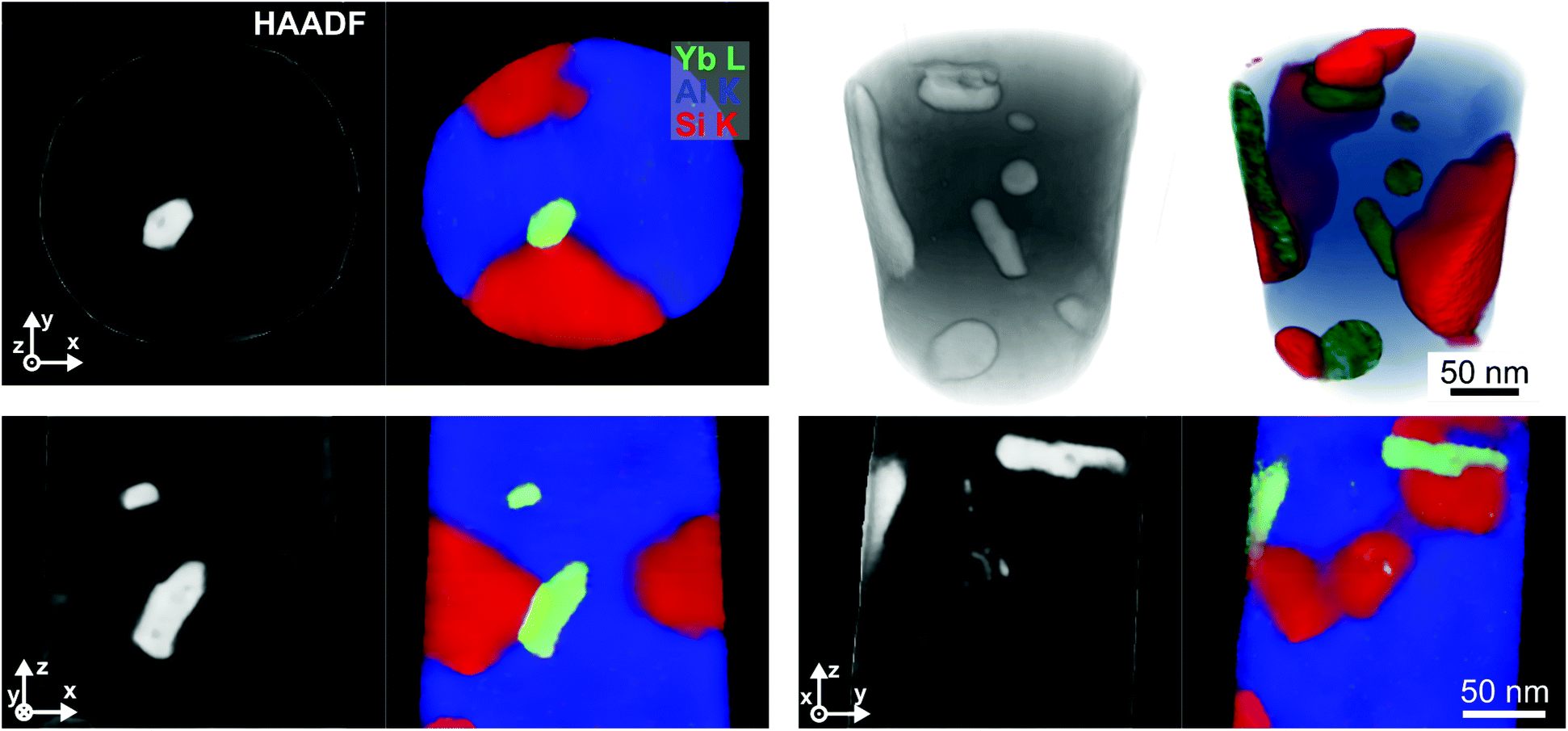 | ||
| Fig. 7 Different slices through correlated reconstructions of the HAADF signal, Yb-, Si- and Al-elemental maps and 3D volume rendering. | ||
Discussion
In both simulations and experiments, we could observe that TGV2 reconstruction is well suited for reconstructing gradual transitions inside a sample, in addition to sharp interfaces. Thereby it extends TV reconstruction, making sparse reconstruction applicable to a wider range of samples. In the investigated sample such gradual transitions are present between Yb-rich and Si-rich precipitates.Linking different signals in the reconstruction significantly improves the quality of analytical STEM reconstructions by transferring morphological information present in the HAADF STEM data to the analytical data and in between the analytical datasets.
Since this transfer is a key feature of our approach, we want to quickly illustrate its inner workings. For simplicity, assume that we have only two channels and consequently the reconstruction approach reduces to
Let us assume that f1 contains far less noise than f2. Then one would naturally choose μ1 greater than μ2, as then f1 is more reliable and thus we make deviation from f1 more expensive. Therefore, the approach finds u1 fitting f1 well, and rather adjusts u2 to obtain common features. This is exactly the effect we observed between the HAADF and Yb reconstructions in the experimental data, where Yb was strongly adjusted to HAADF, but HAADF remained unchanged and in particular was not negatively impacted.
On the other hand, if both channels have the same noise level, and consequently the weights are chosen to be of similar magnitude, deviation from data is equally expensive for both channels, leading to a more balanced compromise in adjusting the reconstructions to obtain common features. This, for example, happens in the reconstruction of the experimental data at the edges between Al and Si, leading to better defined edges for both channels.
Of course, if attaining common features comes at too high a cost, in particular if there actually are no common features in reality, the algorithm will not force common features. So no adjustment appears where it makes no sense to adjust.
In its current implementation, the algorithm will work well for all types of samples which fully remain in the field of view at all tilt angles and is robust to a limited tilt range, cf. ESI Fig. 4.† As such, the algorithm is also readily applicable to samples on a thin-film support, for example, nanoparticles. Only if the sample extends beyond the field of view, problems may arise, similar to other reconstruction algorithms such as SIRT.
The algorithm can be readily applied to any type of signal fulfilling the projection requirement; in particular, its application to EELS data or to combined EDXS/EELS datasets is straightforward.
For the material, the observed gradual transition at the interface between Yb-rich and Si-rich precipitates indicates that a side by side nucleation of the Yb and eutectic Si particles might happen. The diffusion interface between Yb and Si leads to stoichiometry changes (i.e. gradual transitions) of both phases depending on the solute and/or solid diffusion of Yb atoms.
Conclusion
Without the TV-induced bias towards piecewise constant solutions, TGV2 reconstruction achieves high-quality results – and is therefore applicable – for a wide range of materials and will help in understanding their morphology, composition and functionality. The presented linkage of different signals is an ideal approach for obtaining most information out of the available data and can be used for any type of signal used for tomographic reconstruction in a TEM, but the approach is not limited to electron tomography, but can be applied to every type of projection-based tomography. In analytical electron tomography, optimized usage of the available data is mandatory, as the quality and quantity of data which can be acquired in an analytical tomography experiment are severely limited by potential beam damage and acquisition time.Materials and methods
Numerical simulations
In this chapter we give a more detailed description of the phantom data shown in the section Reconstruction of phantom data. To demonstrate the functionality of the joint TGV reconstruction algorithm, we created a multi-channel phantom object. This phantom consists of three channels, which we attribute to the atomic fraction cA of Yb, Al and Si, and has an original size of 2048 × 2048 pixels, with the pixel size being set to 0.1 nm. To obtain a realistic estimation of the number of detector counts for both the EDXS signal and the HAADF signal, we calculated local signal creation probabilities.For the EDXS signal, we used
 | (3) |
The dose De was calculated for an electron current of Ie = 2 nA, a pixel dwell time of tpx = 2 ms and the elemental charge of q = 1.602 × 10⁻¹⁹ C using
 | (4) |
For the zeta-factors, we used  for Si,
  for Al and
  for Yb. Zeta-factors for Si and Al were measured for our microscope; the zeta-factor for Yb is an estimation based on theoretical k-factors for the investigated elements.
To obtain an estimate of the HAADF signal, we used tabulated values of the differential cross section  for elastic scattering from the NIST database,53 integrating them over the angular detector range [θmin,θmax] with54,55
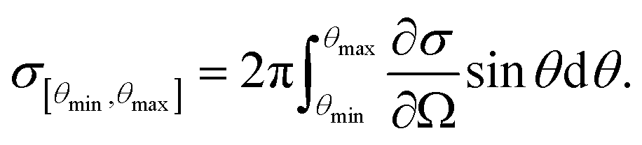 | (5) |
For the inner and outer detector angles, we used θmin = 94.9 mrad and θmax = 188 mrad, which was measured in our system for the Fischione HAADF detector at a camera length of 58 mm.
For each element A, the scattering factor fA was calculated as
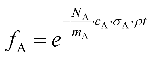 | (6) |
The total HAADF signal was calculated using the scattering factors for all elements and the electron dose De according to
| IHAADF = De(1 − fAl·fSi·fYb). | (7) |
The electron dose is calculated from eqn (4) with Ie = 2 nA and a dwell time of tpx = 2 ms. To account for detector efficiency, we reduce the HAADF signal by a factor of 0.7.
Finally, the phantom data are downscaled from 2048 × 2048 pixels to 305 × 305 pixels using bilinear interpolation, corresponding to a pixel size of 0.67 nm, close to the experimental pixel size. After downscaling, the pixel values are multiplied by a factor of 0.67 to account for the larger thickness of each pixel.
Electron tomography experiments
In this section, we give a more detailed description of the experimental data used in the Experimental reconstruction section. The investigated sample stems from an Al-5 wt% Si alloy with 50 ppm Na and 6100 ppm Yb; a similar sample has been previously analyzed by analytical electron tomography.14 From this material a needle-shaped sample containing Yb- and Si-rich precipitates is prepared using a dual-beam focused ion beam/scanning electron microscope (FIB/SEM) instrument. STEM images are acquired on a probe-corrected FEI Titan3 G2 60-300 microscope operated at 300 kV and equipped with a FEI Super-X four quadrant silicon drift detector (SDD) EDXS system. EDXS spectrum images were acquired every 4° between −74° and +78° at a pixel size 0.76 nm with 276 × 296 pixels. The pixel time was 2 ms, leading to a frame time of 4 min 36 s. The tilt range was limited by the sample holder available at the time of the experiment (a Fischione 2020 Advanced Tomography Holder). Elemental maps of the Al and Si K-lines and of the Yb L-lines are extracted from the EDXS spectrum images. For this purpose, the background is fitted with a Kramers model56 and Gaussian peaks are fitted at all peak positions.Data preprocessing
For the variational reconstruction to work efficiently, the raw sinogram data f need to be consistent with the model. Therefore, the data require suitable preprocessing, and failing to do so could result in artifacts in the reconstructed images. In the ESI† we also discuss the effect of model inconsistencies, which may arise for HAADF STEM data.To correct for sample drift during spectrum image acquisition, the spectrum image is corrected using a linear drift model (constant speed and direction). Drift parameters are calculated by minimizing the difference between the HAADF data acquired during SI (Spectrum Image) acquisition and the fast scan image acquired before. The calculated parameters are used to correct all SI data.57 Alignment of the tilt series is done using the HAADF STEM data. For alignment in the direction of the tilt axis, common-line alignment is applied,58 in the direction perpendicular to the tilt axis the center of mass of each projection is used for alignment and for tilt axis alignment, rotational centers are calculated based on the center of mass.59 The alignment parameters calculated for the HAADF STEM data are applied to all datasets. Drift correction and alignment are done using MATLAB.
Further pre-processing steps can be done using the Python software presented here. Intensity fluctuations can appear between different tilt angles. There are two main sources for these effects: partial shadowing of the detector and residual diffraction contrast. To reduce intensity variations between different projections, we rescale all projections to be non-negative and to have a common mean. This also compensates for partial shadowing of the EDXS detectors. Additionally, projections with very strong diffraction contrast, containing unsatisfactory information, are removed completely.
To correct for non-zero signal values in background regions with no mass (e.g. due to Gaussian noise stemming from the electronics), the corresponding pixels are masked via thresholding and their values are set to zero. A detailed investigation of the impact of data inconsistencies is provided in the ESI.†
Variational modeling
In this section we provide details of the proposed variational model for electron tomography reconstruction, which comprises the solution of (1). For an easier understanding, we describe the reconstruction of a single signal first.Mathematically, this setup can be described as follows: given an angle  (the unit sphere in
 ![[Doublestruck R]](https://www.rsc.org/images/entities/char_e175.gif) 2), the imaging plane is defined as Pθ = {(x, y, z)∈3|(x, y)·θ = 0} and, for given parameters s and z describing the horizontal and vertical offset, respectively, the measurement line Ls,θ,z orthogonal to this imaging plane is given as Ls,θ,z: = {(x′, y′, z′)∈3|(x′, y′)·θ⊥ = s, z′ = z}, where θ⊥ = (θ1, θ2)⊥: = (θ2, −θ1) is a clockwise rotation of θ by 90°. The measurement Tu(s, θ, z) for the parameters (s, θ, z) of a density described by u:3 → is then given as the integration of u over the measurement line Ls,θ,z, i.e.,
2), the imaging plane is defined as Pθ = {(x, y, z)∈3|(x, y)·θ = 0} and, for given parameters s and z describing the horizontal and vertical offset, respectively, the measurement line Ls,θ,z orthogonal to this imaging plane is given as Ls,θ,z: = {(x′, y′, z′)∈3|(x′, y′)·θ⊥ = s, z′ = z}, where θ⊥ = (θ1, θ2)⊥: = (θ2, −θ1) is a clockwise rotation of θ by 90°. The measurement Tu(s, θ, z) for the parameters (s, θ, z) of a density described by u:3 → is then given as the integration of u over the measurement line Ls,θ,z, i.e.,
For any fixed height z, this corresponds to the 2D Radon transform60 of the density u in the plane Pz = {(x, y, z)∈3|x, y∈}. Thus, the measurement operator T corresponds to a slice-wise Radon transform where the image space is parameterized by the height z, the normal of the imaging plane θ and the position in the plane s. The tomographic reconstruction problem then corresponds to solving the equation
| Tu = f |
 | (8) |
Hence, from a Bayesian perspective, the appropriate data discrepancy term in a variational model is the Kullback–Leibler divergence,64 which is for non-negative densities ũ, f (up to constants) given as
 | (9) |
log(0) = 0 and −alog(0) = ∞ for a > 0. For discrete measurements, the integral is replaced by a sum.
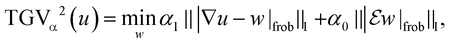
1-type penalization of higher order derivatives via a cascadic decomposition of the unknown. Such a procedure preserves the advantage of the popular Total Variation (TV) functional25 of allowing reconstruction of sharp interfaces while overcoming its defects, particularly its tendency to foster piecewise constant density distributions (the staircasing effect). TGV can be defined for an arbitrary order of differentiation k∈![[Doublestruck N]](https://www.rsc.org/images/entities/char_e171.gif) and for k = 1 coincides with the TV functional. In this work, we employ the second order TGV functional for regularization (k = 2), which, for a single-channel image (or volume) u and parameters α0, α1∈(0, ∞), is given as
and for k = 1 coincides with the TV functional. In this work, we employ the second order TGV functional for regularization (k = 2), which, for a single-channel image (or volume) u and parameters α0, α1∈(0, ∞), is given as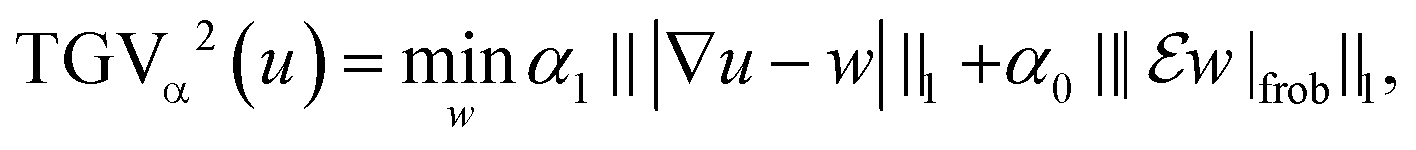 | (10) |
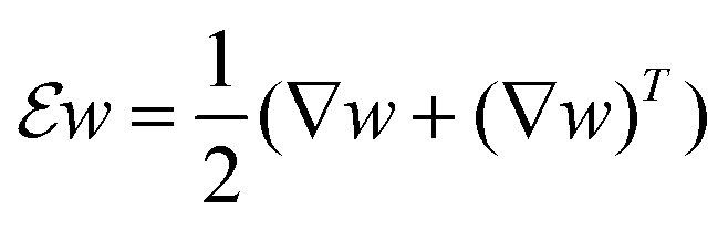 denotes the symmetrized Jacobian matrix. The pointwise norms |·| and |·|frob are the standard Euclidean vector norm and the Frobenius matrix norm, i.e., the root of the sum of squares of all entries of the vector or matrix, respectively.
Thus, TGVα2 minimizes the norm of the gradient while allowing subtraction of a function w, but penalizing this via the norm of the symmetrized Jacobian of w. In particular, in areas with constant u, w can be chosen equal to 0, and in areas with constant ∇u, meaning u is linear, w can be chosen equal to ∇u, such that those areas do not contribute to the TGVα2 functional. Therefore, in reconstructions, TGVα2 promotes piecewise linear solutions, which allow sharp edges to remain intact while allowing linear density gradients, hence maintaining the advantages of TV while overcoming its defects.
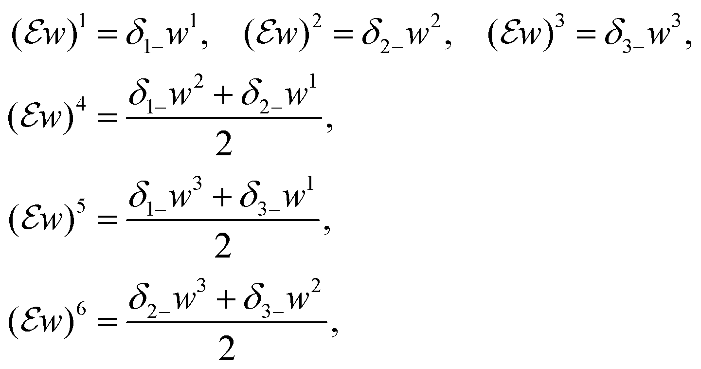
A discretization of TGVα2 is defined according to (10) with the discrete 1 norm, the pointwise Frobenius norms of a vector and a matrix given in the standard way, and discretized differential operators. Denoting by U = N1×N2×N3 the space discrete volumetric densities, the discretized gradient ∇: U → U3 and symmetrized Jacobian 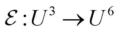 are defined for u∈U and w∈U3, respectively, as ∇u = ((∇u)1, (∇u)2, (∇u)3), where
| (∇u)1 = δ1+u, (∇u)2 = δ2+u, (∇u)3 = δ3+u |
 where
whereand
| δ1+, δ2+, δ3+: U → U and δ1−, δ2−, δ3−: U → U |
 we store each off-diagonal entry only once and, to account for that, count off-diagonal entries twice in the evaluation of the Frobenius norm of
  .
.
 | (11) |
Problem (11) balances the discrepancy between the Radon transform Tu and the data f with the TGVα2(u) regularization, weighted by the regularization parameter μ > 0.
 | (12) |
Note that here, the operators  are applied channel-wise, hence ∇u − w is a matrix field,
  is a tensor field and we use pointwise Frobenius norms for both of them. This corresponds to an 1/2-type penalization and promotes joint sparsity of both ∇u − w and
  , and in particular promotes joint sparsity of the edge sets of all channels. We note that in other studies,46 a similar regularization has been proposed for the joint reconstruction of MR and PET data, where a nuclear-norm based coupling of the first order derivatives was carried out. While the authors reported a slight improvement by using the nuclear norm, the performance was comparable to a Frobenius-norm based penalization and for the sake of simplicity, we employ the latter.
With this multi-channel extension of TGV, we propose the following joint reconstruction model for multi-channel data as an extension of (11):
 | (13) |
Here, different data discrepancies are used for the different measured data sets denoted by fc and each μc weights data fidelity and regularization for the c-th channel. Solving (13) balances the joint regularity of all channels imposed by TGVα2 with the individual channel discrepancies, thus promoting joint edge sets while jointly reconstructing the individual channels. The operators Tc model the measurement operation for each channel and comprise the Radon transform as described above. In this context, we also note that in our experiments all data sets were acquired and reconstructed with the same resolution. Since acquisition of HAADF data is typically much faster than EDXS, an alternative would be to acquire the HAADF signal with a higher resolution and reconstruct all channels at this high resolution. This can be realized in our model by including an additional subsampling operator in the EDXS channels after the Radon transform and would allow a joint reconstruction and zooming of EDXS data.
It is worth mentioning that our method can, of course, also be used to include more information such as EELS data, from which one can expect a further improvement due to additional information present in the data. This will be highly beneficial in cases where elemental maps from EELS data have a better signal-to-noise ratio, or if, for example, valence states are mapped by EELS. We note, however, that assuming the forward operators for EDXS and EELS signals to coincide, such a coupled reconstruction is equivalent to first taking the (weighted) average of the EDXS and EELS signal for each material and then carrying out a reconstruction using the averaged data for the different materials together with the HAADF data.
Numerical solution
In this section we present the derivation and implementation of a solution algorithm for (13), of which the single-channel setting (11) is a special case. For further reference, we note that Graptor – our Python/OpenCL38,39 implementation of the algorithm – as well as a script reproducing all experiments of the paper is available online.37,68 Due to the non-differentiability of the objective functional, we employ a first order primal-dual algorithm66 to solve (13). In order to do so, the problem needs to be reformulated as a saddle-point problem to which the primal-dual algorithm is applicable. To achieve this aim, we first note that TGVα2 can be re-written aswith R(φ,ψ): = α1‖|ϕ|frob‖1 + α0‖|ψ|frob‖1. Also, the constraint uc ≥ 0 for all c can be replaced by adding the functional
 to the energy in (13), where
 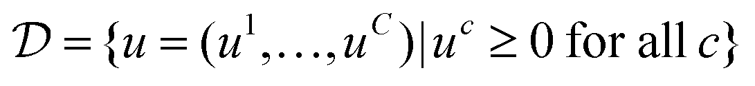 and for any set M we denote
  if u∈M and
  else. Denoting by g* the convex conjugate of a function g, defined as
with (v, ξ) being the scalar product, i.e., the sum of the pointwise products of all entries of v and ξ, we can then rewrite (13) as
 | (14) |
Here, the variables p∈UC×3, q∈UC×6 are the dual variables corresponding to TGVα2, r = (r1, …, rC)∈VC is a dual variable corresponding to the data terms, and
 | (15) |
Hence, problem (13) is equivalent to
 | (16) |
 . With the notion of proximal mappings, i.e.,
the iteration steps of the primal-dual algorithm66 employed for the saddle-point problem (16) for (x,
![[x with combining macron]](https://www.rsc.org/images/entities/i_char_0078_0304.gif) , z) are
, z) are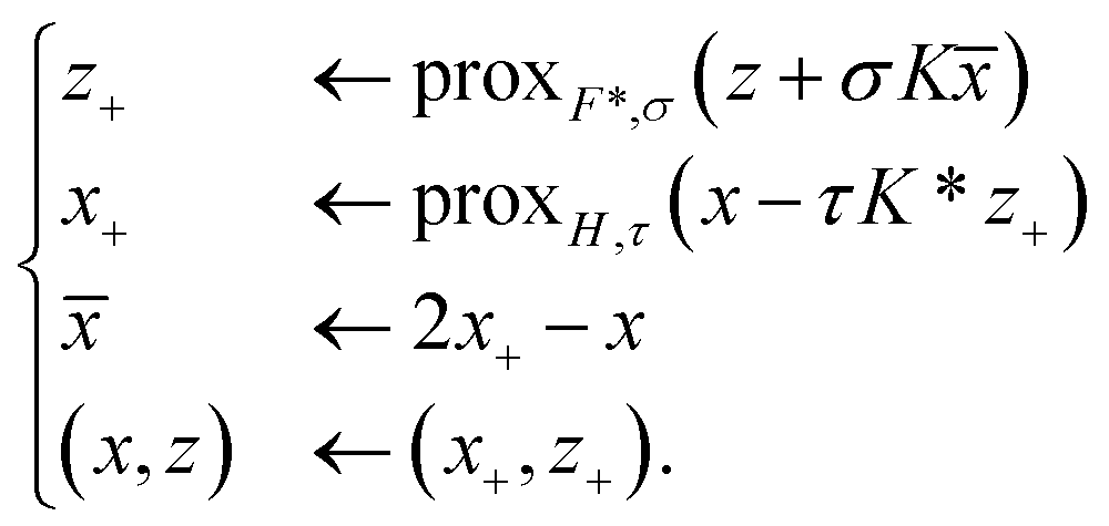 | (17) |
Here, K* denotes the adjoint operator of K and, as a direct computation shows, the proximal mapping of F* decouples component-wise and can be given as
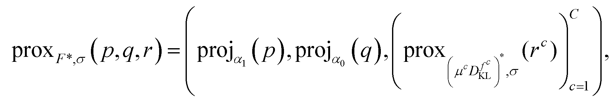
| (projv(r))(x) = r(x)/max(1,|r(x)|frob/v), |
while the proximal mapping of H corresponds again to a projection and is given as
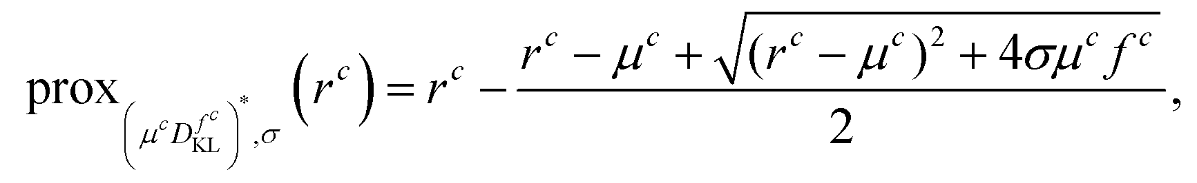
where the maximum is taken point- and component-wise. We also refer the reader to a related study46 for further details of these derivations. For the sake of simplicity, we use the notation
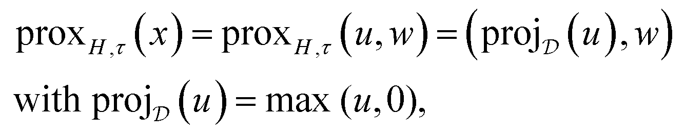
| T*r = (T*rc)Cc=1 |
c denotes the backprojection of rc.
In summary, we can see that, due to our particular reformulation, all iteration steps of Algorithm (17) can be computed explicitly and fast. Furthermore, convergence of the iterate x to a global optimum of (13) can be guaranteed.66 A more explicit formulation of the algorithm can be found in Algorithm 1 below.
| Algorithm 1 | TGV regularized ET reconstruction |
|---|---|
| 1: | function TGV-ET RECONSTRUCTION (f, α, μ) |
| 2: | (T, f) ← normalize (T, f) |
| 3: |
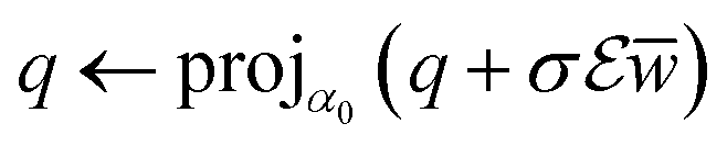
u ← T*f, ū ← u, w ← 0, ![[w with combining macron]](https://www.rsc.org/images/entities/i_char_0077_0304.gif) ← 0, p ← 0, q ← 0, r ← 0 ← 0, p ← 0, q ← 0, r ← 0 |
| 4: | Choose σ > 0 and τ > 0 such that στ‖K‖2 < 1 |
| 5: | repeat |
| 6: |
p ← projα1(p + σ(∇ū − )) |
| 7: |
|
| 8: |
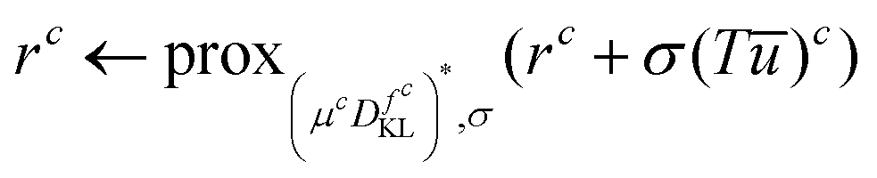 , for c = 1, …, C , for c = 1, …, C |
| 9: |
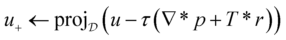
|
| 10: |
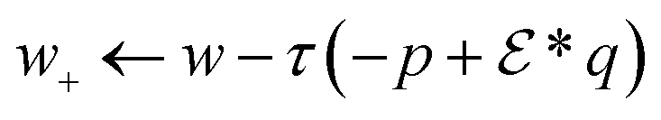
|
| 11: | (ū, ) ← 2(u+, w+) − (u, w) |
| 12: | (u, w) ← (u+, w+) |
| 13: | until Stopping criterion fulfilled |
| 14: | return renormalize (u) |
There, the normalization of the operator T and the corresponding data f in line 2 aims at obtaining an operator with a norm of approximately 1 and data on similar scales, as we found this to improve convergence speed. In order to do so, we estimate the operator norm of T by power iteration,67 divide T by this estimate and rescale the data fc of all channels to the range [0, 1]. Note that, by the nature of the Kullback–Leibler discrepancy, these rescaling operations only affect the choice of the regularization parameter but not the solution set and are reverted with the renormalization step at the end of the algorithm. With rescaled T, the norm ‖K‖ can be estimated from above via straightforward computations by  , allowing σ and τ to be chosen such that στ < 1/17. Although within this constraint, the choice of στ is arbitrary in principle and, in fact, can influence the convergence speed of the algorithm significantly,44 we experienced good convergence behavior with the straightforward choice
 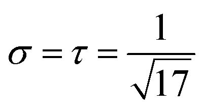 , which was used for all experiments.
As the stopping criterion for Algorithm 1, we used a rather high, predetermined number of 5000 iterations for the experimental and 2000 iterations for the phantom reconstructions such that no relevant change in the iterates was observed beyond this point. A more elaborate stopping criterion that, in some cases, allows to compute the difference of the value of the objective functional to the optimal value could be based on the primal-dual gap of the problem.44 However, this would require some additional computations during the algorithm and for the sake of simplicity and speed, we hence used a fixed number of iterations.
In order to further accelerate the computations, we developed an implementation in Python38via OpenCL39 for multi-core CPUs and Graphical Processing Units (GPUs), which allows for highly parallel execution of all major computations. This is of particular relevance for the forward and backward projections, which are major contributors to the computational effort needed for Algorithm 1 and can be executed completely in parallel, leading to significant speedups.
Tables 2 and 3 illustrate the time required for reconstruction on a computer with an Nvidia(R) GeForce(R) GTX 980 graphic card and an Intel(R) Xeon(R) CPU E5-2690 processor in order to show the computational effort.
| Number of slices | 10 | 30 | ||||
|---|---|---|---|---|---|---|
| Iterations | 500 | 2000 | 5000 | 500 | 2000 | 5000 |
| 1 Channel | 3.03 | 14.79 | 86.93 | 8.13 | 31.84 | 109.19 |
| 4 Channels | 10.98 | 43.27 | 126.87 | 46.51 | 145.08 | 346.17 |
| Iterations | 500 | 2000 | 5000 |
|---|---|---|---|
| N ϕ = 39, N = 296 | 3.03 | 14.79 | 86.93 |
| N ϕ = 39, N = 872 | 22.92 | 93.51 | 235.90 |
| N ϕ = 155, N = 872 | 59.80 | 261.65 | 660.78 |
Regarding the memory requirement, we note that our method in 3D essentially requires to hold, for each channel, 13 variables of image size and two variables of the data size in memory (ignoring temporary storage for computations). In comparison, TV regularization using the same algorithm essentially requires a memory that is 4 times the image size and two times the data size.
The choice of the regularization weights μ = (μ1, …, μC) is more crucial and depends for instance on the noise level of the different measurements, the image resolution and the number of measured angles. Generally, decreasing those parameters leads to increasingly regular and smoothed reconstructions but reduces details, while increasing them provides more details but also increases noise. Nevertheless, as can be observed in Fig. 6, our method is rather robust against suboptimal choices of μ and hence a rough tuning of those parameters should suffice to achieve good results in practice.
A general guideline for choosing those parameters in multi-spectral electron tomography applications is given as follows, where the measurement setup of the paper is used as example. Since the HAADF density data usually contain far less noise than EDXS data, one can first choose the parameter μc corresponding to the HAADF signal, either using our method to first reconstruct only the HAADF signal separately or using some rough, fixed guess for the other parameters.
For the choice of μc for the EDXS channels, remember that these values should roughly correspond to the (unknown) noise levels present in each channel and that channels with similar amounts of noise, e.g., with similar electron counts, should be handled with similar parameters. Motivated by this observation, a heuristic that one can use is to reduce the choice of different μc to the choice of a single parameter ν by setting μc = νξc, where ξc = max(fc). This second, single parameter ν can then again be chosen by visual inspection.
Using this strategy for our experimental data, we first fixed μHAADF = 0.1. Computing the max(fc) then resulted in a ratio of μAl:μSi:μYb = 2.4:1.4:1 and choosing the parameter ν again by visual inspection finally led to the parameters for the EDXS maps given as (μAl, μSi, μYb) = (0.0024, 0.0014, 0.001). A comparison of different settings for the EDXS parameters using this ratio is given in Fig. 6b.
For the parameters used in the reconstruction of the phantom data shown in Fig. 3, we refer the reader to ESI Table 1,† where we used visual comparison of results to determine the parameters.
Finally, we also refer the reader to the ESI† for more information on the parameter choice and the performance of our method in the case of limited angle tomography.
Conflicts of interest
There are no conflicts of interest to declare.Acknowledgements
The Institute of Mathematics and Scientific Computing is a member of NAWI Graz (http://www.nawigraz.at) and BioTechMed Graz (http://www.biotechmed.at). The Institute for Electron Microscopy and Nanoanalysis is also a member of NAWI Graz. KB, MH and RH acknowledge support from the Austrian Science Fund (FWF) (KB, RH: Grant No. P 29192, MH: Grant No. J 4112). RH acknowledges support from the International Research Training Group IGDK 1754 Optimization and Numerical Analysis for Partial Differential Equations with Nonsmooth Structures, funded by the German Research Council (DFG) and the Austrian Science Fund (FWF) [W 1244-N18]. This project has received funding from the European Union's Horizon 2020 research and innovation programme under Grant Agreement No. 823717 ESTEEM3.References
- S. Bals, B. Goris, A. D. Backer, S. V. Aert and G. V. Tendeloo, Atomic resolution electron tomography, MRS Bull., 2016, 41, 525–530 CrossRef.
- J. Miao, P. Ercius and S. J. L. Billinge, Atomic electron tomography: 3D structures without crystals, Science, 2016, 353, aaf2157 CrossRef PubMed.
- R. K. Leary and P. A. Midgley, Analytical electron tomography, MRS Bull., 2016, 41, 531–536 CrossRef.
- P. A. Midgley and M. Weyland, 3D electron microscopy in the physical sciences: the development of Z-contrast and EFTEM tomography, Ultramicroscopy, 2003, 96, 413–431 CrossRef CAS PubMed.
- G. Möbus, R. C. Doole and B. J. Inkson, Spectroscopic electron tomography, Ultramicroscopy, 2003, 96, 433–451 CrossRef.
- M. H. Gass, K. K. K. Koziol, A. H. Windle and P. A. Midgley, Four-Dimensional Spectral Tomography of Carbonaceous Nanocomposites, Nano Lett., 2006, 6, 376–379 CrossRef CAS PubMed.
- G. Haberfehlner, P. Bayle-Guillemaud, G. Audoit, D. Lafond, P. H. Morel, V. Jousseaume, T. Ernst and P. Bleuet, Four-dimensional spectral low-loss energy-filtered transmission electron tomography of silicon nanowire-based capacitors, Appl. Phys. Lett., 2012, 101, 063108 CrossRef.
- K. Jarausch, P. Thomas, D. N. Leonard, R. Twesten and C. R. Booth, Four-dimensional STEM-EELS: Enabling nano-scale chemical tomography, Ultramicroscopy, 2009, 109, 326–337 CrossRef CAS PubMed.
- L. Yedra, A. Eljarrat, R. Arenal, E. Pellicer, M. Cabo, A. López-Ortega, M. Estrader, J. Sort, M. D. Baróe, S. Estradé and F. Peiró, EEL spectroscopic tomography: Towards a new dimension in nanomaterials analysis, Ultramicroscopy, 2012, 122, 12–18 CrossRef CAS PubMed.
- B. Goris, L. Polavarapu, S. Bals, G. Van Tendeloo and L. M. Liz-Marzán, Monitoring Galvanic Replacement Through Three-Dimensional Morphological and Chemical Mapping, Nano Lett., 2014, 14, 3220–3226 CrossRef CAS PubMed.
- A. Genc, L. Kovarik, M. Gu, H. Cheng, P. Plachinda, L. Pullan, B. Freitag and C. Wang, XEDS STEM tomography for 3D chemical characterization of nanoscale particles, Ultramicroscopy, 2013, 131, 24–32 CrossRef CAS PubMed.
- K. Lepinay, F. Lorut, R. Pantel and T. Epicier, Chemical 3D tomography of 28nm high K metal gate transistor: STEM XEDS experimental method and results, Micron, 2013, 47, 43–49 CrossRef CAS PubMed.
- T. J. A. Slater, A. Macedo, S. L. M. Schroeder, M. G. Burke, P. OBrien, P. H. C. Camargo and S. J. Haigh, Correlating Catalytic Activity of AgAu Nanoparticles with 3D Compositional Variations, Nano Lett., 2014, 14, 1921–1926 CrossRef CAS PubMed.
- G. Haberfehlner, A. Orthacker, M. Albu, J. Li and G. Kothleitner, Nanoscale voxel spectroscopy by simultaneous EELS and EDS tomography, Nanoscale, 2014, 6, 14563–14569 RSC.
- T. J. A. Slater, R. S. Bradley, G. Bertali, R. Geurts, S. M. Northover, M. G. Burke, S. J. Haigh, T. L. Burnett and P. J. Withers, Multiscale correlative tomography: an investigation of creep cavitation in 316 stainless steel, Sci. Rep., 2017, 7, 7332 CrossRef CAS PubMed.
- M. Sanna Angotzi, A. Musinu, V. Mameli, A. Ardu, C. Cara, D. Niznansky, H. L. Xin and C. Cannas, Spinel Ferrite CoreShell Nanostructures by a Versatile Solvothermal Seed-Mediated Growth Approach and Study of Their Nanointerfaces, ACS Nano, 2017, 11, 7889–7900 CrossRef CAS PubMed.
- A. Orthacker, G. Haberfehlner, J. Tändl, M. C. Poletti, B. Sonderegger and G. Kothleitner, Diffusion Defining Atomic Scale Spinodal Decomposition within Nano-Precipitates, Nat. Mater., 2018, 17(12), 1101–1107 CrossRef CAS PubMed.
- P. Torruella, R. Arenal, F. de la Peña, Z. Saghi, L. Yedra, A. Eljarrat, L. López-Conesa, M. Estrader, A. López-Ortega, G. Salazar-Alvarez, J. Nogués, C. Ducati, P. A. Midgley, F. Peiró and S. Estradé, 3D Visualization of the Iron Oxidation State in FeO/Fe3O4 Core-Shell Nanocubes from Electron Energy Loss Tomography, Nano Lett., 2016, 16, 5068–5073 CrossRef CAS PubMed.
- Z. Saghi, D. J. Holland, R. Leary, A. Falqui, G. Bertoni, A. J. Sederman, L. F. Gladden and P. A. Midgley, Three-Dimensional Morphology of Iron Oxide Nanoparticles with Reactive Concave Surfaces. A Compressed Sensing-Electron Tomography (CS-ET) Approach, Nano Lett., 2011, 11, 4666–4673 CrossRef CAS PubMed.
- B. Goris, S. Bals, W. Van den Broek, E. Carbó-Argibay, S. Gómez-Graña, L. M. Liz-Marzán and G. Van Tendeloo, Atomic-scale determination of surface facets in gold nanorods, Nat. Mater., 2012, 11, 930–935 CrossRef CAS PubMed.
- O. Nicoletti, F. de la Peña, R. K. Leary, D. J. Holland, C. Ducati and P. A. Midgley, Three-dimensional imaging of localized surface plasmon resonances of metal nanoparticles, Nature, 2013, 502, 80–84 CrossRef CAS PubMed.
- A. Hörl, G. Haberfehlner, A. Trügler, F.-P. Schmidt, U. Hohenester and G. Kothleitner, Tomographic reconstruction of the photonic environment of plasmonic nanoparticles, Nat. Commun., 2017, 8, 37 CrossRef PubMed.
- B. Goris, W. Van den Broek, K. J. Batenburg, H. Heidari Mezerji and S. Bals, Electron tomography based on a total variation minimization reconstruction technique, Ultramicroscopy, 2012, 113, 120–130 CrossRef CAS.
- R. Leary, Z. Saghi, P. A. Midgley and D. J. Holland, Compressed sensing electron tomography, Ultramicroscopy, 2013, 131, 70–91 CrossRef CAS PubMed.
- L. I. Rudin, S. Osher and E. Fatemi, Nonlinear total variation based noise removal algorithms, Physica D, 1992, 60, 259–268 CrossRef.
- L. Donati, M. Nilchian, S. Trépout, C. Messaoudi, S. Marco and M. Unser, Compressed sensing for STEM tomography, Ultramicroscopy, 2017, 179, 47–56 CrossRef CAS PubMed.
- D. J. Holland and L. F. Gladden, Less is More: How Compressed Sensing is Transforming Metrology in Chemistry, Angew. Chem., Int. Ed., 2014, 53, 13330–13340 CrossRef CAS PubMed.
- N. Monsegue, X. Jin, T. Echigo, G. Wang and M. Murayama, Three-Dimensional Characterization of Iron Oxide (α-Fe2O3) Nanoparticles: Application of a Compressed Sensing Inspired Reconstruction Algorithm to Electron Tomography, Microsc. Microanal., 2012, 18, 1362–1367 CrossRef CAS PubMed.
- S. C. Crawford, S. Ermez, G. Haberfehlner, E. J. Jones and S. Gradecak, Impact of nucleation conditions on diameter modulation of GaAs nanowires, Nanotechnology, 2015, 26, 225604 CrossRef PubMed.
- D. Zanaga, T. Altantzis, L. Polavarapu, L. M. Liz-Marzán, B. Freitag and S. Bals, A New Method for Quantitative XEDS Tomography of Complex Heteronanostructures, Part. Part. Syst. Charact., 2016, 33, 396–403 CrossRef CAS.
- Z. Zhong, B. Goris, R. Schoenmakers, S. Bals and K. J. Batenburg, A bimodal tomographic reconstruction technique combining EDS-STEM and HAADF-STEM, Ultramicroscopy, 2017, 174, 35–45 CrossRef CAS PubMed.
- K. Bredies, K. Kunisch and T. Pock, Total Generalized Variation, SIAM J. Imaging Sci., 2010, 3, 492–526 CrossRef.
- K. Bredies and M. Holler, Regularization of linear inverse problems with total generalized variation, J. Inverse Ill-Posed Probl., 2014, 22, 871–913 Search PubMed.
- K. Bredies, Efficient Algorithms for Global Optimization Methods in Computer Vision, Springer Berlin Heidelberg, 2014, vol. 8293, pp. 44–77 Search PubMed.
- Z. Zhong, W. J. Palenstijn, J. Adler and K. J. Batenburg, EDS tomographic reconstruction regularized by total nuclear variation joined with HAADF-STEM tomography, Ultramicroscopy, 2018, 191, 34–43 CrossRef CAS PubMed.
- Z. Zhong, W. J. Palenstijn, N. R. Vigan and K. J. Batenburg, Numerical methods for low-dose EDS tomography, Ultramicroscopy, 2018, 194, 133–142 CrossRef CAS PubMed.
- R. Huber, M. Holler and K. Bredies, Graptor [Software], Zenodo, 2019, DOI:10.5281/zenodo.2586204.
- Python programming language, https://www.python.org/ Search PubMed.
- OpenCL programming standard, https://www.khronos.org/opencl/ Search PubMed.
- F. Knoll, K. Bredies, T. Pock and R. Stollberger, Second order total generalized variation (TGV) for MRI, Magn. Reson. Med., 2011, 65, 480–491 CrossRef PubMed.
- I. Chatnuntawech, A. Martin, B. Bilgic, K. Setsompop, E. Adalsteinsson and E. Schiavi, Vectorial total generalized variation for accelerated multi-channel multi-contrast MRI, Magn. Reson. Imaging, 2016, 34, 1161–1170 CrossRef PubMed.
- T. Valkonen, K. Bredies and F. Knoll, Total generalized variation in diffusion tensor imaging, SIAM J. Imaging Sci., 2013, 6, 487–525 CrossRef.
- M. Schloegl, M. Holler, A. Schwarzl, K. Bredies and R. Stollberger, Infimal convolution of total generalized variation functionals for dynamic MRI, Magn. Reson. Med., 2017, 78, 142–155 CrossRef CAS PubMed.
- K. Bredies and M. Holler, A TGV-based framework for variational image decompression, zooming and reconstruction. Part II: Numerics, SIAM J. Imaging Sci., 2015, 8, 2851–2886 CrossRef.
- W. Guo, J. Qin and W. Yin, A New Detail-Preserving Regularization Scheme, SIAM J. Imaging Sci., 2014, 7, 1309–1334 CrossRef.
- F. Knoll, M. Holler, T. Koesters, R. Otazo, K. Bredies and D. Sodickson, Joint MR-PET reconstruction using a multi-channel image regularizer, IEEE Trans. Med. Imaging, 2017, 36, 1–16 Search PubMed.
- M. Holler, R. Huber and F. Knoll, Coupled regularization with multiple data discrepancies, Inverse Probl., 2018, 34, 084003 CrossRef PubMed.
- A. Al-Aleef, A. Alekseev, I. MacLaren and P. Cockshott, 31st Picture Coding Symposium, Cairns, Australia, 2015.
- P. Gilbert, Iterative methods for the three-dimensional reconstruction of an object from projections, J. Theor. Biol., 1972, 36, 105–117 CrossRef CAS.
- W. J. Palenstijn, J. Bédorf, J. Sijbers and K. J. Batenburg, A distributed ASTRA toolbox, Adv. Struct. Chem. Imaging, 2016, 2, 19 CrossRef PubMed.
- W. van Aarle, W. J. Palenstijn, J. Cant, E. Janssens, F. Bleichrodt, A. Dabravolski, J. D. Beenhouwer, K. J. Batenburg and J. Sijbers, Fast and flexible X-ray tomography using the ASTRA toolbox, Opt. Express, 2016, 24, 25129–25147 CrossRef PubMed.
- M. Watanabe and D. B. Williams, The quantitative analysis of thin specimens: a review of progress from the Cliff-Lorimer to the new ζ-factor methods, J. Microsc., 2006, 221, 89–109 CrossRef CAS PubMed.
- A. Jablonski, F. Salvat, C. J. Powell and A. Y. Lee, NIST Electron Elastic-Scattering Cross-Section Database Version 4.0, NIST Standard Reference Database Number 64, National Institute of Standards and Technology, Gaithersburg MD, 20899, 2016 Search PubMed.
- F. Banhart, Irradiation effects in carbon nanostructures, Rep. Prog. Phys., 1999, 62, 1181–1221 CrossRef CAS.
- G. S. Khandelwal and E. Merzbacher, Displacement Cross Sections for Fast Electrons Incident on Gold, Phys. Rev., 1963, 130, 1822–1825 CrossRef CAS.
- H. Kramers, On the Theory of X-ray Absorption and Continuous X-ray Spectrum, Philos. Mag., 1923, 46, 836 CAS.
- G. Haberfehlner, P. Thaler, D. Knez, A. Volk, F. Hofer, W. E. Ernst and G. Kothleitner, Formation of bimetallic clusters in superfluid helium nanodroplets analysed by atomic resolution electron tomography, Nat. Commun., 2015, 6, 8779 CrossRef CAS PubMed.
- T. Printemps, G. Mula, D. Sette, P. Bleuet, V. Delaye, N. Bernier, A. Grenier, G. Audoit, N. Gambacorti and L. Hervé, Self-adapting denoising, alignment and reconstruction in electron tomography in materials science, Ultramicroscopy, 2016, 160, 23–34 CrossRef CAS PubMed.
- S. G. Azevedo, D. Schneberk, J. Fitch and H. Martz, Calculation of the rotational centers in computed tomography sinograms, IEEE Trans. Nucl. Sci., 1990, 37, 1525–1540 CrossRef.
- S. Helgason, The Radon Transform, Birkhäuser Basel, 1999 Search PubMed.
- K. Hahn, H. Schndube, K. Stierstorfer, J. Hornegger and F. Noo, A comparison of linear interpolation models for iterative CT reconstruction, Med. Phys., 2016, 43, 6455–6473 CrossRef PubMed.
- T. Furnival, R. K. Leary and P. A. Midgley, Denoising time-resolved microscopy image sequences with singular value thresholding, Ultramicroscopy, 2017, 178, 112–124 CrossRef CAS PubMed.
- D. Rossouw, P. Burdet, F. J. de la Peña, C. Ducati, B. R. Knappett, A. E. H. Wheatley and P. A. Midgley, Multicomponent Signal Unmixing from Nanoheterostructures: Overcoming the Traditional Challenges of Nanoscale X-ray Analysis via Machine Learning, Nano Lett., 2015, 15(4), 2716–2720 CrossRef CAS PubMed.
- T. Hohage and F. Werner, Inverse problems with Poisson data: statistical regularization theory, applications and algorithms, Inverse Probl., 2016, 32, 093001 CrossRef.
- K. Bredies and M. Holler, A TGV-based framework for variational image decompression, zooming and reconstruction. Part I: Analytics, SIAM J. Imaging Sci., 2015, 8, 2814–2850 CrossRef.
- A. Chambolle and T. Pock, A First-Order Primal-Dual Algorithm for Convex Problems with Applications to Imaging, J. Math. Imaging Vis., 2011, 40, 120–145 CrossRef.
- S. Börm and C. Mehl, Numerical Methods for Eigenvalue Problems, De Gruyter, 2012 Search PubMed.
- G. Haberfehlner and G. Kothleitner, EDX Electron Tomography Dataset on AlSiYb-Alloy [Data set], Zenodo, 2019 DOI:10.5281/zenodo.2578865.
Footnotes |
| † Electronic supplementary information (ESI) available: Analysis of the impact of data inconsistencies and preprocessing, parameter choices used for the phantom data, depiction of the individual EDX projections for the experimental data, comparison of regularization parameters for SIRT reconstructions, analysis of the impact of a limited tilt-angle range on reconstructions, quantitative analysis via mean to standard deviation maps, and computational evaluation of the Radon transform implementation. See DOI: 10.1039/C8NR09058K |
| ‡ It should be noted that as one channel we denote one type of dataset to be reconstructed, such as the HAADF signal or a single EDXS elemental map, meaning if we consider sinograms for HAADF, EDX aluminum, EDX silicon and EDX ytterbium, then C = 4. This should not be confused with spectral channels in EDXS or EELS. |
| This journal is © The Royal Society of Chemistry 2019 |