High-precision potassium isotopic analysis by MC-ICP-MS: an inter-laboratory comparison and refined K atomic weight

Abstract

In the last a few years, several groups proposed new methods of high-precision K isotope analysis using Multiple Collector Inductively Coupled Plasma Mass Spectrometer (MC-ICP-MS) either through “collision gas” or “cold plasma” methods. Here we report a detailed method analyzing K isotopes in high-precision using Neptune Plus MC-ICP-MS in cold plasma and conduct an inter-laboratory comparison. The precision of measurements of ⁴¹K/³⁹K ratios of a single run in this study can routinely reach ∼0.05 per mil (95% confidence interval; n = 10). The long-term (20 months) robustness and reproducibility of this method have also been evaluated (0.11 per mil; 2 standard deviation; n = 890). We also report K isotopic compositions of 20 geological reference materials and compare this method with recent methods from other laboratories. These independent measurements of the same reference materials agree well with each other within reported analytical uncertainties. Because of the newly improved methods and observed K isotopic fractionation among reference materials, the International Union of Pure and Applied Chemistry (IUPAC) recommended values for the weight of potassium and the atomic fractions of K isotopes need to be revised.

---

1. Introduction

Potassium is an alkali metal and a lithophile element in geochemistry. It is highly enriched in the Earth's crust, and the average K₂O content of the upper continental crust is 2.8 wt%, making it the eighth most abundant element.¹ It is a major constituent in common minerals in granites such as feldspars and micas. It also exists as relatively pure KCl form in sylvite deposits as the result of evaporation of ancient seawater, which is the major industrial source of K.² During weathering, K can be leached out from igneous rocks, and K⁺ ions can be readily incorporated into clay minerals in the soils such as illites. Potassium concentration is low in river water: about 2.3 ppm on average,³ while that in seawater is 399 ppm.^4,5 In the mantle, K is incompatible and mostly present as a trace element. The bulk K abundance in the mantle is estimated as 260 ppm, which is about two orders of magnitude lower than that in the crust.⁶ Potassium is also proposed to be present in the core; however the core composition is less constrained and whether there is any K in the core is still largely unknown.^7,8

Potassium has two stable isotopes, ³⁹K (93.2581%) and ⁴¹K (6.7302%), and one naturally occurring radioactive isotope ⁴⁰K (0.0117%) with a long half-life (t_1/2 = 1.277 × 10⁹ years). The K stable isotopic composition is typically expressed in delta notation, where δ⁴¹K = ([(⁴¹K/³⁹K)_sample/(⁴¹K/³⁹K)_standard − 1] × 1000). The branched decay of ⁴⁰K to ⁴⁰Ca and ⁴⁰Ar is an essential radioactive heating source and may have been even more important than U and Th in the early Earth. It may also be the possible energy source that kick-started the geodynamo, which produces the magnetic field of the Earth.^8–10 The K–Ca–Ar system is also useful in chronology and is one of the most popular dating tools. The precise determination of K isotopic ratios (⁴⁰K/³⁹K) and the understanding of the K stable isotope fractionation among minerals would help to further improve the accuracy of K–Ca–Ar geochronology.

The natural variation of K isotopic compositions was not well known until very recent. The earliest measurements of potassium isotopic ratios were done with Dempster style mass spectrographs in 1920–30s.^11–13 Brewer¹⁴ was the first to investigate the variation of K isotopic compositions among rocks, minerals and plants. This and many other studies in this era concluded that although there is measurable isotopic difference among biological samples (e.g., normal vs. cancerous tissues), the K isotopic variations of geological samples are negligible.^14–24 Taylor and Urey²⁵ successfully fractionated K isotopes by chemical exchange with zeolites; while Brewer²⁶ didn't observe any K isotopic fractionation during evaporation experiments. After decades of relative inactivity, studies on K isotopes resumed in the 1970s.^27–34 These investigations covered various types of samples, including terrestrial samples such as basalts, granites and mantle xenoliths, and extraterrestrial samples such as chondrites, eucrites, and lunar samples, especially after the return of Apollo missions. The major discovery during this period is that lunar regolith is significantly enriched in heavier K isotopes (i.e., ⁴¹K), and this observation was interpreted as volatilization and partial loss of K during the micro-meteorite impacting and solar wind sputtering on the surface of the Moon.^27,31,35 Most of these studies were conducted on Thermal Ionization Mass Spectrometers (TIMS), and the error bars of these early measurements are typically larger than 1% (relative precision here and after) for ⁴¹K/³⁹K ratios.³⁴

Humayun and Clayton^36,37 made a major contribution to the K isotope systematics of both terrestrial and extraterrestrial samples achieving the best analytical precision (0.5 per mil for ⁴¹K/³⁹K ratio) at the time by using the Secondary Ion Mass Spectrometer (SIMS) technique. Intriguingly, there was still no detectable K isotopic difference between meteoritic, lunar, and terrestrial samples (except for lunar regoliths as had been discovered previously), even though there is a clear trend of volatile depletion as indicated by K/U ratios between the most primitive chondrites and the highly depleted Moon and Vesta. Potassium isotope studies were also carried out on tektites and microtektites using SIMS,^38,39 and there were no detectable K isotopic differences between tektites on average and their possible source materials. Although experiments showed that kinetic isotope fractionation processes such as evaporation and thermal (Soret) diffusion would produce measurable K isotopic fractionation,^40–42 no such fractionation has been observed in natural samples such as chondrules that exhibit loss of alkali metal volatiles including K.^43,44

During the last two decades, the fast development of Multiple-Collector Inductively-Coupled-Plasma Mass-Spectrometry (MC-ICP-MS) has made it possible to improve the analytical precisions of many isotopic systems dramatically.^45–48 The importance of K isotopes and the lack of high-precision K isotopic data have been realized by the geochemistry community. Morgan et al. pioneered the development of a high-precision K isotopic analytical method using MC-ICP-MS.^49–52 More recent endeavors have also been made by Santiago Ramos and Higgins,⁵³ Wang and Jacobsen,^54,55 Li et al.,^56,57 Morgan et al.,⁵⁸ Santiago Ramos et al.,⁵⁹ Hu et al.⁶⁰

Here we report a method using a Thermo Scientific Neptune Plus MC-ICP-MS to further push the analytical limits on K isotope measurements and to test the long-term (20 month) robustness and reproducibility of such method. We also report a detailed procedure of ion-exchange chromatography to purify K with low blanks. We apply this protocol to 20 well-studied reference materials in various petrology and mineralogy to survey the range of K isotopic fractionation between igneous and sedimentary rocks and minerals, and also for the purpose of inter-laboratory comparison and calibration.

2. Chemistry

2.1. Sample description

As high-precision K isotope analysis has not been possible until last a few years, there has been very limited high-quality data available so far. Samples in this study were thus selected on the basis of the following two criteria: (1) availability of data reported by previous studies of high-precision K isotopes by other methods; or (2) samples that are well-documented and could provide a broad range of various types of igneous and sedimentary rocks and minerals. Therefore, we selected 20 reference materials provided by USGS (U.S. Geological Survey), ANRT (Association Nationale de la Recherche Technique, Paris), and NIST (National Institute of Standards and Technology). Among these 20 samples, the K isotopic compositions of 5 reference materials (BCR-1, BHVO-2, AGV-1, G-2 and GSP-1) have been previously reported by recent studies,^54,56,58,60 which can be used to verify our data. Between 10 and 50 mg of each sample was dissolved with a two-step procedure (HF/HNO₃ and HCl/HNO₃ mixtures; see Table 1) in Parr general-purpose acid digestion vessels, depending on the sample's K concentration.

Table 1 Sample digestion and potassium column purification protocols

Sample dissolution protocol
1	Weigh 10–50 mg of each sample by electronic balance (depending on each sample's K concentration)
2	Dissolve samples in concentrated HF/HNO3 mixture (VHF : VHNO3 ∼ 3 : 1)
3	Heat in Parr high-pressure digestion vessels at 150 °C in Fisher Scientific Isotemp 500 oven for two days
4	Evaporate the digested samples completely under heat lamps
5	Re-digest the samples by HCl/HNO3 mixture (VHCl : VHNO3 ∼ 3 : 1)
6	Evaporate the samples again under heat lamps

---

Big column purification
1	Big columns (ID = 1.5 cm, BIO-RAD Econo-Pac) filled with 17 mL AG50-X8 100–200 mesh cation-exchange resin
2	Resin cleaning: 100 mL 6 mol L^−1 HCl
3	Resin conditioning: 50 mL 0.7 mol L^−1 HNO3
4	Load sample: the samples are digested in 1.1 mL 0.7 mol L^−1 HNO3. After centrifuging the solution, load 1 mL supernatant onto the big columns
5	Matrix eluted by adding 82 mL 0.7 mol L^−1 HNO3
6	Pre-cut: 5 mL 0.7 mol L^−1 HNO3 to monitor the recovery of K
7	K-cut: potassium collected in Teflon beakers by addition of 107 mL 0.7 mol L^−1 HNO3
8	Post-cut: 5 mL 0.7 mol L^−1 HNO3 to monitor the recovery of K
9	Purified solutions are dried down under heat lamps overnight for small column

---

Small column purification
1	Small columns (ID = 0.5 cm, BIO-RAD glass Econo-column) filled with 2.4 mL AG50-X8 100–200 mesh cation-exchange resin
2	Resin cleaning: 20 mL 6 mol L^−1 HCl
3	Resin conditioning: 15 mL 0.5 mol L^−1 HNO3
4	Load sample: the samples are digested in 1 mL 0.5 mol L^−1 HNO3, then loaded all onto the small columns
5	Matrix eluted by adding 14 mL 0.5 mol L^−1 HNO3
6	Pre-cut: 2 mL 0.5 mol L^−1 HNO3 to monitor the recovery of K
7	K-cut: potassium collected in Teflon beakers by addition of 18 mL 0.5 mol L^−1 HNO3
8	Post-cut: 2 mL 0.5 mol L^−1 HNO3 to monitor the recovery of K
9	Purified solutions are dried down under heat lamps overnight for analysis

---

The 20 samples include 11 igneous rocks, 7 sedimentary rocks, and 2 potassium-rich minerals. They have been well studied and are readily available to other groups for future inter-laboratory comparison. The igneous rocks used in this study include three basalts from three tectonic settings: a continental flood basalt (BCR-1), a mid-ocean ridge basalt (BIR-1) and an ocean island basalt (BHVO-2). We also investigated one andesite (AGV-2), two granites (GS-N and G-2), one granodiorite (GSP-1), one quartz latite (QLO-1), one rhyolite (RGM-1), one tonalite (TLM-1), and one obsidian (NIST-278). Two pure K-bearing minerals were also studied: one sodium feldspar (NIST-99a) and one potassium feldspar (FK-N). The sedimentary rocks used in this study include one limestone (NIST-1c), two sediments (NIST-2704 and BSK-1), one marine mud (MAG-1), and three shales (SCo-1, SDO-1 and SGR-1). The sample names, petrological types, locations and literature data are listed in Table 2.

Table 2 Potassium isotopic compositions of igneous, sedimentary rocks and minerals

Sample name	Type	Location	Distributed by^a	K (%) this study	K (%) literature^b	δ^41K SRM3141a (‰)	95% C.I.^c	n
a USGS = U.S. Geological Survey; ANRT = Association Nationale de la Recherche Technique (Paris); NIST = U.S. National Institute of Standards and Technology. b The K concentrations are from ref. 63 except that the K concentration of TLM-1 and BSK-1 is from ref. 62 and those of AGV-1, BCR-1, BHVO-2, BIR-1, G-2, RGM-1 are from ref. 71. c 95% confidence interval. d Number of measurements.
Mafic
BCR-1	Basalt	Portland, Oregon	USGS		1.44	−0.49	±0.05	8
BHVO-2	Basalt	Hawaiian Volcanic Observatory	USGS		0.43	−0.46	±0.04	13
BIR-1	Basalt	Reykjavík, Iceland	USGS	0.025	0.024	−0.51	±0.06	9
Intermediate
AGV-1	Andesite	Lake County, Oregon	USGS		2.44	−0.43	±0.08	10
Felsic
GS-N	Granite	Senones, Vosges, France	ANRT	4.03	3.84	−0.43	±0.08	13
G-2	Granite	Bradford, Rhode Island	USGS		3.74	−0.46	±0.04	19
GSP-1	Granodiorite	Silver Plume, Colorado	USGS	3.56	4.57	−0.44	±0.05	10
QLO-1	Quartz latite	Lake County, Oregon	USGS	3.15	2.99	−0.40	±0.04	11
RGM-1	Rhyolite	Glass Mountain, Siskiyou County, California	USGS	3.68	3.56	−0.35	±0.04	16
TLM-1	Tonalite	Side County, California	USGS	1.38	1.31	−0.46	±0.06	16
278	Obsidian	Clear Lake, Newberry Crater, Oregon	NIST	3.16	3.45	−0.36	±0.07	12
Mineral
99a	Feldspar, sodium	Spruce pine pegmatite district of North Carolina	NIST	3.98	4.30	−0.08	±0.08	9
FK-N	Feldspar, potassium	Tamil Nadu, India	ANRT	8.37	10.63	−0.26	±0.09	8
Sedimentary
1c	Limestone, argillaceous	Putnam County, Indiana	NIST	0.25	0.23	−0.58	±0.03	14
2704	River sediment	Buffalo River, Buffalo, New York	NIST	1.67	2.00	−0.41	±0.05	9
BSK-1	Sediment	Kesterson National Wildlife Refuge, California	USGS	2.16	2.30	−0.37	±0.05	15
MAG-1	Marine mud	Wilkinson Basin, Gulf of Maine	USGS	2.17	2.95	−0.44	±0.04	13
SCo-1	Shale	Natrona County, Wyoming	USGS	2.33	2.30	−0.43	±0.04	16
SDO-1	Shale	Morehead, Kentucky	USGS	2.56	2.78	−0.22	±0.08	9
SGR-1	Oil shale	Green River formation, Wyoming	USGS	1.02	1.38	−0.26	±0.06	10
Other
Suprapur	99.995% purity KNO3		Merck KGaA			0.00	±0.04	14
Blank K	Total-procedure blank					−1.31	±0.08	4

---

2.2. Ion-exchange chromatography

We applied a two-step procedure of the ion-exchange column chromatography to purify K from silicate matrix. This procedure was first proposed by Strelow et al.,⁶¹ and later adopted by Humayun and Clayton,^36,37 and recently by Wang and Jacobsen,⁵⁴ and Li et al.⁵⁶ Here we are using a modified procedure, which has been detailed in Table 1. The column calibration curve is shown in Fig. 1.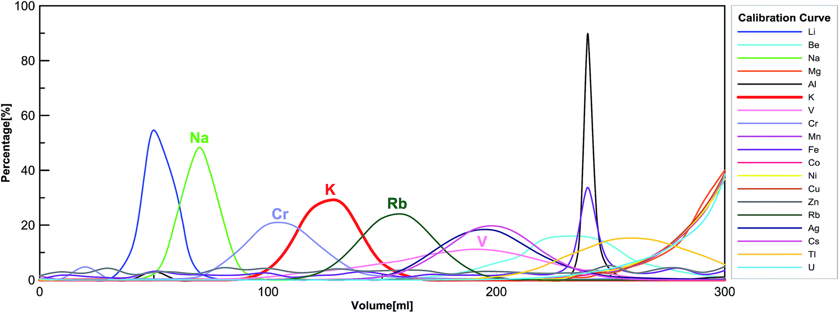

Fig. 1 Big-column calibration using reference material BHVO-2 in 0.7 mol L⁻¹ HNO₃ (see Table 1 for details).

The first column is a BIO-RAD Econo-Pac column (1.5 cm ID, polypropylene) filled with 17 mL AG50-X8 100–200 mesh cation-exchange resin. Columns were first cleaned with 100 mL 6 mol L⁻¹ double-distilled HCl and then conditioned with 50 mL 0.7 mol L⁻¹ double-distilled HNO₃. After centrifuging, samples dissolved in 1 mL 0.7 mol L⁻¹ HNO₃ were loaded onto the first columns. Matrix elements were eluted by adding 82 mL 0.7 mol L⁻¹ HNO₃ and then pre-cuts were collected into disposable polypropylene tubes by adding 5 mL 0.7 mol L⁻¹ HNO₃. Potassium was recovered into acid-cleaned Teflon beakers by adding 107 mL 0.7 mol L⁻¹ HNO₃. Post-cuts were collected into additional disposable polypropylene tubes by adding 5 mL 0.7 mol L⁻¹ HNO₃. The recovered K was dried down and redissolved with 1 mL 0.5 mol L⁻¹ HNO₃ before loading onto the second column.

The second column is a BIO-RAD Econo column (0.5 cm ID, borosilicate glass) filled with 2.4 mL AG50-X8 100–200 mesh cation-exchange resin. Columns were first cleaned with 20 mL 6 mol L⁻¹ double-distilled HCl and then conditioned with 15 mL 0.5 mol L⁻¹ double-distilled HNO₃. All 1 mL samples were loaded onto the second columns. Matrix elements were eluted by adding 14 mL 0.5 mol L⁻¹ HNO₃ and then pre-cuts were collected into disposable polypropylene tubes by adding 2 mL 0.5 mol L⁻¹ HNO₃. Potassium was recovered into acid-cleaned Teflon beakers by adding 18 mL 0.5 mol L⁻¹ HNO₃. Post-cuts were collected into additional disposable polypropylene tubes by adding 2 mL 0.5 mol L⁻¹ HNO₃. The recovered K was dried down and redissolved with 2% HNO₃ before measuring with the mass spectrometers.

2.3. Blanks and yield

With this procedure, improved compared to our previous one,⁵⁴ we are able to use less acid (thus less blank contamination) and shorten the time of bench work. We use double-distilled HCl and HNO₃ from trace metal grades. The acid distillation was done with two Savillex DST-1000 acid purification systems for both HCl and HNO₃. We have tested the total-procedure blanks seven times on six different columns following the exact same procedure as normal samples. The average of the seven total-procedure blanks is 0.26 ± 0.15 μg (2SD; n = 7). The total-procedure blank in this study is three times lower (0.26 μg vs. 0.82 μg) than that in the previous study.⁵⁴ We cannot measure the K isotopic composition of the blank K after one total-procedure because there is not enough K to prepare a 1 mL solution at 1 ppm. As such, we combined six total-procedure blanks into one, so we were able to prepare a 4 mL solution at 300 ppb and match it to a 300 ppb standard. We were then able to measure this combined blank four times (1 mL needed for each individual analysis). The result is shown in Table 2. The K isotopic composition of total-procedure blanks is very different (−1.31 ± 0.05‰) from that of any natural samples that having been analyzed. The blank K likely comes from distilled acids, Milli-Q water, and Teflon beakers, and this extremely fractionated K isotopic composition is possible due to kinetic fractionation processes during the distillation of acids. Regardless of its source, the blank K contamination would introduce a small error to the K isotopic analysis due to its distinct isotopic composition.

For our analysis, we need at least 10 μg K for ten measurements (1 μg K for each measurement: 1 ppm solution × 1 mL). For most samples, we aim for 100 μg K or more to be used for repeat measurements and for suppressing the blank contamination. In the minimal case of 10 μg K from the sample, the sample/blank ratio is 38. Assuming that the K isotopic composition of the blank is −1.31 per mil (in delta notation), the blank contamination will introduce a ∼0.03 per mil error (≈−1.31/38), which is well below the analytical uncertainty of our K isotope measurements. For most samples with >100 μg K, the sample/blank ratio is above 385, and thus the influences from the blank contamination are negligible. Low-blank chemistry is especially crucial for any low-K samples; fortuitously, most terrestrial crustal rocks are high in K abundance, and the blank contamination is negligible for all samples in this study.

We ensure that the yields of all samples through the column chemistry are more than 99% by monitoring the pre-cuts and post-cuts for both steps of the column chemistry. The concentrations of K in pre-cuts, post-cuts, and K-cuts of each sample were measured with a Thermo Scientific iCAP Q quadrupole ICP-MS. The yield of each sample is calculated as

Yield = (C_K-cut × V_K-cut)/(C_pre-cut1 × V_pre-cut1 + C_post-cut1 × V_post-cut1 + C_pre-cut2 × V_pre-cut2 + C_post-cut2 × V_post-cut2 + C_K-cut × V_K-cut)

The C_pre-cut1, C_post-cut1, C_pre-cut2, and C_post-cut2 represent concentrations of K in the pre-cuts and post-cuts collected during the first and second steps of column chemistry. The C_K-cut represents the concentrations of the final K solution collected after the second column. The V_K-cut, V_pre-cut1, V_post-cut1, V_pre-cut2, V_post-cut2 are the final volumes of these solutions.

We also compare the K concentrations of the sample calculated from the final K-cuts and sample weights to the K concentrations reported in the literature.^62,63 Considering the potential sample loss during digestion and transfer between containers and errors from weighing, pipetting and the quadrupole ICP-MS analysis, the K concentrations of the sample analyzed in this study agree well with the literature data within 10% (see Table 2). Both the calculated yields and this comparison to literature data confirm that we had collected ∼100% K from the samples and there is no possible isotopic fractionation via column chemistry.

2.4. Isotopic fractionation of K during ion-exchange column chemistry

We also evaluate the isotope fractionation by column chemistry if the K recovery rate is not 100%. We passed two aliquots of the standard NIST SRM3141a through two big columns. As shown in ESI Table S1,† for column 1 we collected 108 mL 0.5 mol L⁻¹ HNO₃ as described in our routine method (see Table 1). In contrast, for column 2, we collected six 18 mL fractions of the 108 mL 0.7 mol L⁻¹ HNO₃. We then measured the K concentrations and K isotopic compositions of the seven column test samples. The results are shown in ESI Table S1† and Fig. 2. The column 1, where we collected 100% K, has a K isotopic composition of −0.02 ± 0.04‰, which is indistinguishable from the expected value (0.00 ± 0.05‰; by definition). For column 2, none of the six fractions have the correct value for NIST SRM3141a. For example, the first 18 mL fraction contains only 2% of all K, but its K isotopic composition is very different (1.17 ± 0.07) from the isotopic composition of NIST SRM3141a. Our result for isotopic fractionation of K during column chemistry agrees well with similar tests in previous studies.^37,58 Even though each fraction is fractionated in K isotopes, the calculated total for the six fractions (−0.06 ± 0.04‰) is indistinguishable from the expected value (0.00 ± 0.05‰). We also calculated the subtotal for the first five fractions of the six, the last five fractions of the six, and the middle four fractions. These subtotals show that even if we do not collect 100% K, the incomplete collection of K during the column chemistry will not introduce a fractionation more than 0.08‰ (see ESI Table S1†), which is slightly larger than our routine analytical uncertainty within a single run session and is smaller than our long-term reproducibility. Nevertheless, we always ensure the >99% recovery rate via monitoring pre-cuts and after-cuts of the column chemistry. The column fractionation test above is just to evaluate the possible isotopic fractionation that a column can produce when a ∼100% recovery rate is not achieved.

Fig. 2 Result of column fractionation tests. The shaded area is the isotopic composition of the standard by definition (0.00 ± 0.05‰; 95% C.I.).

3. Mass spectrometry

3.1. Potassium isotopic determination

Measurements of K isotopes with MC-ICP-MS have been challenging due to large argon-based interferences (³⁸Ar¹H⁺ on ³⁹K⁺ and ⁴⁰Ar¹H⁺ on ⁴¹K⁺). Two methods were previously proposed to alleviate or eliminate this problem (see Fig. 3): (1) the “cold plasma” method, which reduces ArH⁺ ions in the plasmas by lowering the RF generator power;^{49–52,58,60,64} and (2) the “collision gas” method, which dissociates the molecular ions by introducing a collisional gas (He) or reaction gas (H₂/D₂).^{40,41,54–57,65–69} We have previously developed a high-precision K isotope measurement protocol based on the “collision gas” method using a GV Instruments IsoProbe MC-ICP-MS equipped with a hexapole collision gas cell at Harvard University.⁵⁴ In this study, we test the “cold plasma” method with a Thermo Scientific Neptune Plus MC-ICP-MS. Compared to the IsoProbe, the Neptune Plus MC-ICP-MS has many advantages, including significantly increased mass resolution, higher sensitivity, and better stability; additionally, the Neptune Plus MC-ICP-MS is much more widely-available than IsoProbe MC-ICP-MS. Hence, this protocol of high-precision K isotope analysis would be more accessible than our previous method.⁵⁴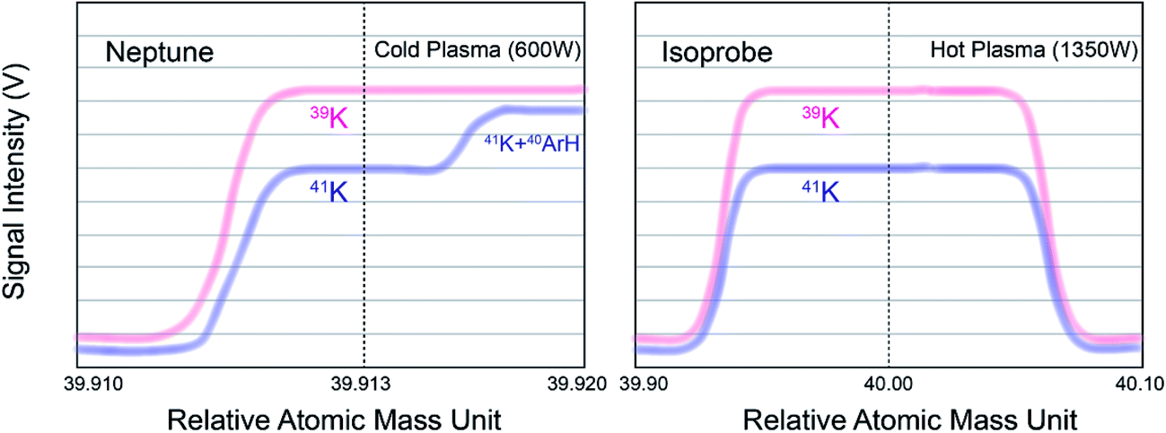

Fig. 3 Schematic drawings of the peak shapes in the two methods of K isotope measurements by MC-ICP-MS. The Ar-interference-free shoulder is about 0.003–0.004 a.m.u. (atomic mass unit). The peak position and shape of Neptune are stable and it only moves ∼0.001 a.m.u. every 24 hour session.

This “cold plasma” method relies on Neptune Plus' pseudo-high resolution (no total separation of the two peaks) to resolve the mass difference between ⁴¹K and ⁴⁰Ar¹H⁺ at a cold plasma condition. At regular ICP-MS operation state (high RF forward power of ∼1350 W), Ar⁺ and ArH⁺ are the major background peaks. At lower RF forward power (∼600 W or less), NO⁺ is the primary ion observed, while the Ar⁺ and ArH⁺ signals can be attenuated dramatically.⁶⁴ In addition, because the ³⁸Ar/⁴⁰Ar is naturally extremely low, the interference of ³⁸Ar¹H⁺ on ³⁹K can be neglected in this situation. The interference of ⁴⁰Ar¹H⁺ on ⁴¹K can be resolved at the “shoulder” of the peak (see Fig. 3).

Because the “cold plasma” mode would considerably suppress the intensities of potassium isotopes, we use an APEX Ω high sensitivity desolvation system produced by Elemental Scientific as the sample introduction system to increase the signal intensity. The typical parameters of the MC-ICP-MS and APEX Ω desolvation system are listed in Table 3. With this configuration, we can achieve ∼15 V for ³⁹K at 1 ppm concentration, which is comparable to what we previously achieved with the “collision gas” method.⁵⁴ All measurements were done with sample-standard bracketing technique, and the standard we used here is NIST SRM3141a.

Table 3 Instrument settings on the Neptune Plus MC-ICP-MS and APEX Ω

MC-ICP-MS parameters
RF power	600 W
Cool gas flow rate	15 L min^−1
Intermediate gas flow rate	1.0 L min^−1
Sample gas flow rate	1.15 L min^−1
Focus quad	− 5.5 V
Dispersion quad	0.00 V
Integration time	8.389 s
Number of integrations	1
Number of cycles	25
Number of blocks	1
Cup configuration	L2 (^39K), L1 (^40Ar), Center (^41K), H3 (^44Ca)
APEX Ω parameters
H2 flow rate	10 mL min^−1
Ar (sweep gas) flow rate	10 L min^−1
Sample uptake rate	100 μL min^−1
Spray chamber temperature	140 °C
Peltier cooler temperature	3 °C
Desolvator temperature	155 °C

---

We measure each sample ∼10 times at 1 ppm concentration (±1%), and the averages of the ∼10 measurements are reported. The internal (within-run) reproducibility (95% confidence interval) of ∼10 measurements is given for each sample in Table 2, and the typical internal reproducibility is ∼0.05‰. The external reproducibility is calculated as the 2 standard deviations (2SD) of the measured aliquots of same reference materials (BHVO-2 and G-2) that passing through six columns (see Table 4). The typical external reproducibility (2SD) is ∼0.08‰. This analytical precision is also comparable to that of “collision gas” methods reported in literature.^54,56

Table 4 Potassium isotopic compositions of analytical tests of the column chemistry

	δ^41K SRM3141a (‰)	95% C.I^a	n
a 95% confidence interval. b Number of measurements.
BHVO-2 (basalt)
Column 1	−0.54	±0.10	10
Column 2	−0.46	±0.07	9
Column 3	−0.44	±0.10	10
Column 4	−0.46	±0.05	10
Column 5	−0.43	±0.06	9
Column 6	−0.49	±0.08	10
Average	−0.47
2SD	0.08
G-2 (granite)
Column 1	−0.50	±0.08	10
Column 2	−0.43	±0.07	8
Column 3	−0.47	±0.08	9
Column 4	−0.45	±0.14	8
Column 5	−0.48	±0.08	10
Column 6	−0.53	±0.07	8
Average	−0.48
2SD	0.07

---

3.2. Standard

At this time, there is no certified isotopic standard for potassium available. Previously, NIST SRM985 was the certified isotopic standard used to determine the natural isotopic abundance of potassium;^32,70 however, it is no longer available. Conventionally, single-element standards (Suprapur and NIST SRM999b, SRM3141a) have been used for K isotope studies. Humayun and Clayton^36,37 used Merck KGaA Suprapur® 99.995% purity potassium nitrate (KNO₃) and Wang and Jacobsen⁵⁴ purchased and used the nominally same standard from Merck KGaA. However, this newly-purchased Merck KGaA Suprapur® 99.995% KNO₃ may not from the same batch, and hence its K isotopic composition is not guaranteed to be identical to the one used by Humayun and Clayton.^36,37 In contrast, both Morgan et al.⁵⁸ and Li et al.⁵⁶ chose to use the NIST SRM 999b or 3141a as their standards. However, NIST SRM 999b or 3141a is also not a certified isotopic standard, but rather a concentration standard, which means it cannot be guaranteed that each batch will have the same K isotopic composition.

In this study, we measured the K isotopic compositions of both the Merck KGaA Suprapur® 99.995% KNO₃ and the NIST SRM3141a (see Table 2). We found that these two standards are indistinguishable from each other in term of K isotopes. This result is not coincidental or surprising since both standards might have been produced from the same industrial source of sylvite deposits. This identity of Suprapur KNO₃ and the NIST SRM3141a is fortunate because we can directly compare the data from these four groups^{50–52,54–56,60} without conversion. However, for future analysis, we suggest further inter-laboratory calibrations of the standards used by different institutions.

3.3. Matrix effects

One drawback of this “cold plasma” method is that “matrix effects” are enhanced due to the overall low abundance of background ions.⁶⁴ Thus, the substantial presence of matrix elements (other than K) would affect the K signal intensities measured by MC-ICP-MS. We use the sample-standard bracketing technique, in which the standard is a high-purity K solution (no matrix element) whereas the sample is a silicate rock after purification by ion exchange chromatography (containing trace amounts of matrix elements). Therefore, uneven matrix effects in standards and samples would induce large analytical artifacts.

In order to eliminate the matrix effects, a two-step column chromatography procedure has been implemented. We have checked the elemental compositions of all samples with a Thermo Scientific iCAP Q quadrupole ICP-MS after running the sample through the two-step column procedure. In rare cases, the only interference element present after two columns is chromium. According to the calibration curves of the AG50-X8 100–200 mesh cation-exchange resin in 0.7 mol L⁻¹ HNO₃ (see Fig. 1), the Cr peak has an overlap with the K peak. Other major rock-forming elements such as Ca, Fe, and Mg do not fall into the K cut (see Fig. 1).

We tested the matrix effect of Cr by doping different amounts of Cr (1, 2, 5, and 10% relative to K). The result in this study is shown in ESI Table S2† and Fig. 4, where we also plotted the matrix effect of Mg, Al, Ca, Ti, V, Cr and Rb reported in literature.^56,58,60 We found that when matrix elements are <2% in solution, no resolvable matrix effects are observed in K isotopes. This matrix effect needs to be monitored and it is critical for any samples with relatively low K concentrations. If more than 2% matrix element is found in the final K solutions, additional column chemistry is needed to purify the K in the samples further.

Fig. 4 Potassium isotopic compositions of standards doped with potential residual matrix elements (Mg, Al, Ca, Ti, V, Cr and Rb) measured by this study and in literature.^54,58,60 Both “cold plasma” and “collision gas” methods produce no measurable matrix effects for samples containing less than 2% matrix elements.

3.4. Long-term reproducibility

As discussed above, we measure each sample ∼10 times and report the averages of the ∼10 repeat measurements. The internal (within-run) reproducibility (95% confidence interval; 95% C.I.) of ∼10 measurements is typically ∼0.05‰. In order to evaluate the long-term reproducibility of this high-precision K isotopic method by MC-ICP-MS, we have been routinely analyzing the reference material BHVO-2 during many analytical sessions. As shown in Fig. 5, we have accumulated 90 days' data of BHVO-2 over 20 months from Jan. 2017 to Aug. 2018 including 890 individual analyses. During each day's session, we analyze BHVO-2 5–15 times depending on the number of other samples. The total average of all 890 analyses is −0.480 ± 0.006‰ (95% C.I.) which agrees well with the Bulk Silicate Earth (BSE) value (−0.479 ± 0.027‰; 2SD) reported by Wang and Jacobsen.⁵⁴ The 2 standard deviations (2SD) of the 90 days' sessions of BHVO-2 over 20 months is 0.11‰. This value represents the long-term reproducibility of this K isotopic method, which is comparable to what has recently been reported by another group (0.17‰).⁵⁸

Fig. 5 K isotopic compositions of reference material BHVO-2 measured in 90 days over 20 months from Jan. 2017 to Aug. 2018 (890 individual analyses). Each data point represents the average of 5–15 measurements of BHVO-2 during a 24 hour analytical session. Error bars represent the 95% confidence interval of repeated analyses during each 24 hour analysis session. The grand average of all 890 analyses is −0.480 ± 0.006‰ (95% C.I.) which agrees well with the Bulk Silicate Earth (BSE) value (−0.479 ± 0.027‰; 2SD) defined by basalts from three different tectonic settings.⁵⁴

4. Results

All the K isotopic compositions measured in this study are presented in Table 2 and Fig. 6. In addition to the isotopic data, we also report the K concentrations (after column chemistry) of these samples (Table 2). For comparison, the concentrations from literature are also included.^62,63,71 The concentrations measured in this study in general agree well with the literature data and verify the ∼100% recovery rates of the column chemistry (which are also supported by measuring the pre-cuts and after-cuts collected during column chemistry).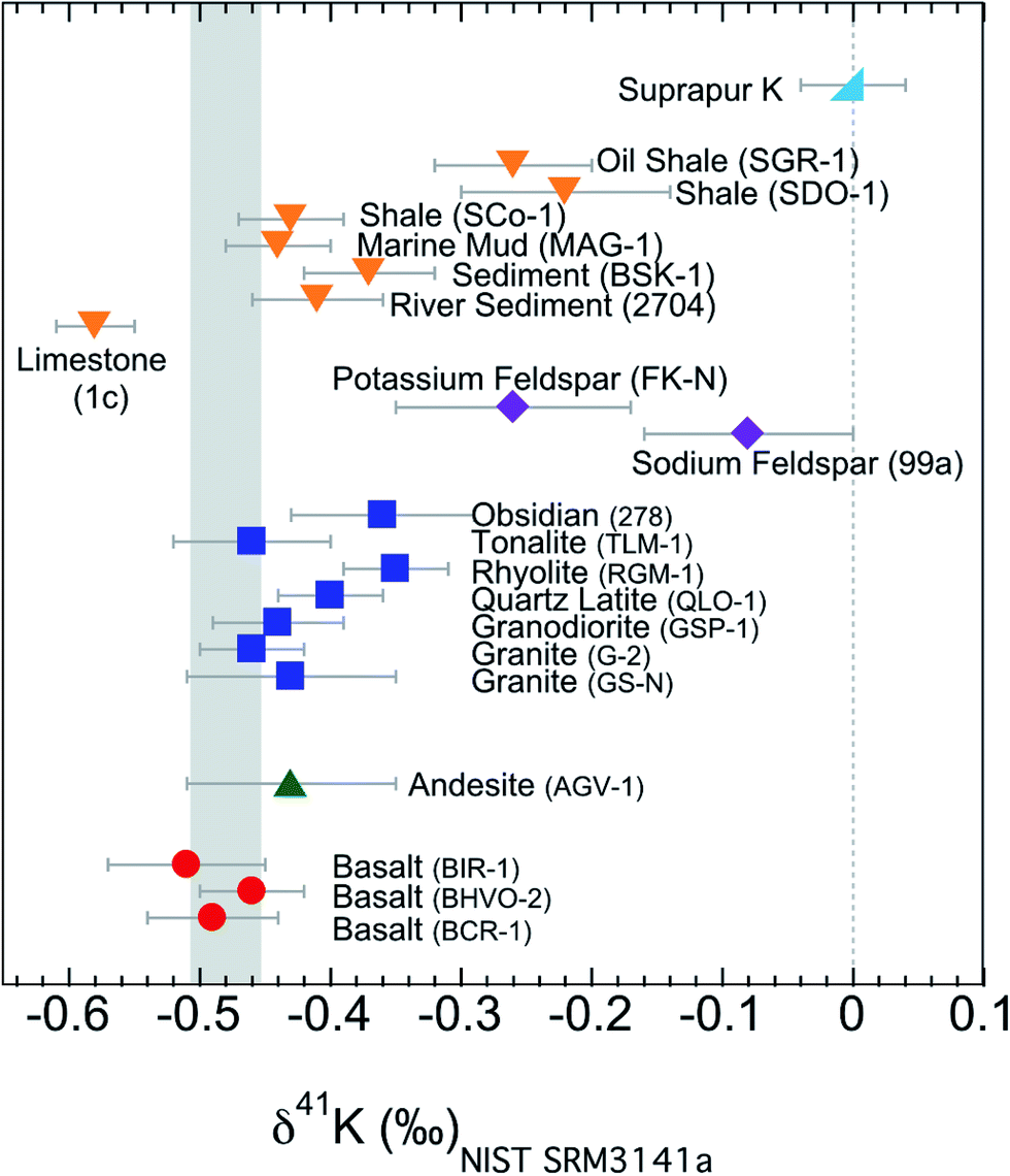

Fig. 6 K isotopic compositions of all samples in this study. Error bars represent the 95% confidence interval of about 10 repeated analysis. Igneous rocks have a confined range of variation in K isotopes, while sedimentary rocks have a much larger variation. The shaded area is the Bulk Silicate Earth (BSE) value (−0.48 ± 0.03‰) defined by basalts from three different tectonic settings.⁵⁴

4.1 Igneous rocks and minerals

The K isotopes in igneous rocks in this study range from −0.51 ± 0.05‰ to −0.35 ± 0.04‰. The average of three basalts (continental flood, mid-ocean ridge and ocean island basalts) is −0.49 ± 0.05‰ (2SD), which is indistinguishable from the Bulk Silicate Earth (BSE) value (−0.48 ± 0.03‰) defined by basalts from three different tectonic settings.⁵⁴ All mafic and intermediate igneous rocks and most of the felsic igneous rocks have an indistinguishable K isotope composition (igneous average= −0.45 ± 0.07‰; 2SD; n = 9). This igneous average is also indistinguishable from the BSE value.⁵⁴

The only two igneous rock samples that are different from the BSE value are also the two samples with the highest SiO₂ contents (see Fig. 7): one rhyolite from Glass Mountain, Siskiyou County, California (RGM-1) and one obsidian from Clear Lake, Newberry Crater, Oregon (NIST 278). These two high-Si felsic samples have K isotopic compositions of −0.35 ± 0.04‰ and −0.36 ± 0.06‰, which are significantly heavier than the igneous average (−0.45 ± 0.07‰) reported in this study. As also shown in Fig. 6, the K isotopic compositions of felsic rocks do exhibit slightly heavier values than those of mafic rocks.

Fig. 7 K isotopic compositions of all igneous rocks in this study versus their SiO₂ abundances. The SiO₂ data are from literature.⁷⁴ The shaded area is the Bulk Silicate Earth (BSE) value (−0.48 ± 0.03‰) defined by basalts from three different tectonic settings.⁵⁴ Although most igneous rocks are indistinguishable from this BSE value, two high-Si felsic igneous rocks (rhyolite and obsidian) are significantly enriched in heavy K isotopes.

The two minerals (NIST 99a and FK-N) from the igneous rocks, sodium and potassium feldspars, have even larger K isotopic fractionations relative to the BSE value than bulk samples. The sodium feldspar from Spruce Pine pegmatite district of North Carolina (NIST 99a) has the heaviest K isotopic composition in this study. It is consistent with the observation by Morgan et al.⁵⁸ that pegmatites (consisting of feldspars as the major K phases) show >1‰ K isotopic fractionation.

In summary, most igneous rocks (mafic, intermediate and felsic) have the same K isotopic composition, which agrees well with the BSE value previously defined from the average of basalts (mid-ocean ridge basalt, ocean island basalt, and continental flood basalt). However, we have also observed that two high-Si (degassing-influenced) felsic rocks (rhyolite and obsidian) and two K-rich minerals (sodium and potassium feldspars) are significantly enriched in heavy K isotopes. This variation observed between different rocks and minerals indicates that high-temperature K isotope fractionations are finally resolvable with the new high-precision K isotope analysis method.

4.2 Sedimentary rocks

Compared to that of igneous rocks, the range of K isotopic variations is much broader among sedimentary rocks: from −0.58 ± 0.03‰ to −0.22 ± 0.07‰ (see Fig. 6). These values are significantly different from those of igneous rocks. Except for the argillaceous limestone, all sedimentary rocks give values that are slightly higher than the BSE value. The argillaceous limestone from Putnam County, Indiana (NIST 1c) is significantly below the BSE value, and defines the lowest value measured in this study. On the other end, two shales (SDO-1 and SGR-1) have the heaviest K isotopic compositions of all sedimentary rocks while another shale (SCo-1) is indistinguishable from most igneous rocks. One sediment from Kesterson National Wildlife Refuge, California (BSK-1) is significantly higher than igneous rocks, while the river sediment from Buffalo River, New York (NIST 2704) and one marine mud (MAG-1) are also indistinguishable from igneous rocks. In general, the K isotope compositions of sedimentary rocks have a much larger range of variation and show a different pattern from that of igneous rocks. Relative to the BSE composition, the K isotope compositions of sedimentary rocks could be either enriched or depleted in heavy K isotopes. This observation indicates that although there is only limited K isotopic fractionation during high-temperature magmatic processes, K isotopes readily fractionate during various low-temperature aqueous processes.

5. Discussion

5.1 Inter-laboratory comparison of K isotope data by different instrumentation

After the published work done by Humayun and Clayton,^36,37 there have been few K isotope studies because of the analytical challenge they presented until the past few years. Two new methods of high-precision K isotopic analysis have been used by several laboratories as described above in Sections 1 and 3.^{50–52,54,56,60} To compare data collected by different methods and by different laboratories, we must first establish an inter-laboratory calibration method in order to confirm that there are no artificial errors or systematical shifts between different groups.

The first issue is the different standards used by different laboratories: Merck KGaA Suprapur® 99.995% KNO₃, NIST SRM 999b, and NIST SRM 3141a. As discussed above in Section 3.2, none of these standards are ideal for isotopic analysis because they are not certified isotopic standards; however, they are the only presently available choices. We measured both Suprapur and NIST 3141a standards in this study (see Table 2 and Fig. 6), and we found no resolvable difference in terms of K isotopes within the current typical analytical errors (∼±0.05‰). Regardless, more effort should be made in the future to coordinate between research laboratories so that the same isotopic standard of K is used by all groups. At this time, however, it is acceptable to use either Merck KGaA Suprapur® 99.995% KNO₃ or the NIST SRM3141a, since they have no measurable difference in the K isotopic composition.

The second issue is that different laboratories use different methods to remove the Ar based interference; see Section 3.1 for a description of both the “cold plasma” and “collision gas” methods. It has not been rigorously tested whether these two methods would produce a systematic consistency in measuring ⁴¹K/³⁹K ratios. It needs to be verified that the data produced using one method agrees well with data produced using the other when analyzing the same sample. We have measured K isotopes using both the “cold plasma” and “collision gas” methods.⁵⁴ Here we analyzed five USGS standards (BCR-1, BHVO-2, AGV-1, GSP-1, and G-2) in this study, which are the only ones that have been reported by different groups.^{54–56,58,60} As shown in Fig. 8, our results measured with the “cold plasma” or “collision gas” method are indistinguishable from those data measured by different groups using different methods.^{54–56,58,60} The new data show that both methods, using either Isoprobe, Neptune Plus or Nu Plasma MC-ICP-MS, produce data that are comparable to each other.

Fig. 8 K isotopic compositions of reference materials measured in this study using the “cold plasma” method and literature data using “cold plasma” and “collision gas” method.^{54–56,58,60} Error bars represent the 95% C.I. (Confidence Interval) for this study and literature data. The shaded area is the Bulk Silicate Earth (BSE) value (−0.48 ± 0.03‰) defined by basalts from three different tectonic settings.⁵⁴

In summary, the high-precision K isotopic compositions measured with both “cold plasma” and “collision gas” methods relative to both Merck KGaA Suprapur® 99.995% KNO₃, and NIST SRM 3141a in the literature can be compared directly. There is no systematic shift found between data from different laboratories.

5.2 Revision of the weight of K and the atomic fractions of K isotopes

Because of the lack of K isotopic fractionation in natural samples, the recommended values for the atomic weight of K and the atomic fractions of K isotopes published by the International Union of Pure and Applied Chemistry (IUPAC) have not been modified since 1979.^70,72 Due to the discovery of measurable K isotopic fractionation among natural samples in the past several years, beginning with Morgan et al.,⁴⁹ it is necessary to recalculate these values of the atomic weight of K and the atomic fractions of K isotopes. The current IUPAC values are based on the TIMS measurements of the K isotopic standard NIST-SRM985 by Garner et al.³² Recently, Naumenko et al.⁷³ proposed an improved measurement of ⁴⁰K/³⁹K of NIST-SRM985; thus we suggest to update the absolute isotopic compositions of NIST-SRM985 by combining both results.^32,73 However, the K isotopic composition of the standard NIST-SRM985 is not equal to those of natural samples (such as seawater, silicate rocks, and chondrites). The natural abundances of K isotopes and the atomic weight of K need to reflect those of natural samples rather than those of the artificial standard NIST-SRM985.

We calculated the absolute abundances of K isotopes and the atomic weight of K in seawater and the Bulk Silicate Earth based on the absolute abundances of K isotopes measured in NIST-SRM985 and relative differences between NIST-SRM985 and the seawater and the Bulk Silicate Earth (see Table 5). Notably, the value of the atomic weight of K in Bulk Silicate Earth is revised from 38.0983 to 38.0982 a.m.u. (atomic mass unit). The newly calculated atomic weight of K agrees with the one proposed recently by Morgan et al.⁵⁸ However, the new atomic fractions of K isotopes of the Bulk Silicate Earth are different between two groups due to (1) the slightly different (yet same within errors) estimates for the Bulk Silicate Earth value, and (2) different estimates of ⁴⁰K abundance. Morgan et al.⁵⁸ used the current IUPAC value for ⁴⁰K abundance,^70,72 while in this study we propose to use the more precise value from Naumenko et al.⁷³ In addition, we also report the newly calculated absolute abundances of K isotopes and the atomic weight of K in the CI chondrite and the Bulk Silicate Moon (see Table 5). Therefore, we suggest IUPAC to revise their recommended values for absolute abundances of K isotopes and the atomic weight of K.

Table 5 Atomic weight of potassium and the atomic fractions of potassium isotopes in natural samples

	Measured ^39K/^41K	Measured ^40K/^41K	Measured ^40K/^39K	Measured δ^41K SRM985^a (‰)	^39K (atomic fraction)	^40K (atomic fraction)	^41K (atomic fraction)	Atomic weight
a The data were converted from the original in the literature through the 0.259 per mil difference between NIST-SRM985 and seawater measured by ref. 58.
NIST-SRM985
Garner et al.^32	13.85662	0.0017343			0.932581073	0.000116722	0.067302205	39.0983
Naumenko et al.^73			0.000125116
IUPAC^70					0.932581	0.000117	0.067302	39.0983
Garner et al.^32 + Naumenko et al.^73					0.932581112	0.000116681	0.067302207	39.0983
Seawater^58				−0.259	0.932597383	0.000116667	0.067285950	39.0983
Bulk Silicate Earth ^54				−0.838	0.932633759	0.000116637	0.067249604	39.0982
CI chondrite^55				−0.893	0.932637214	0.000116634	0.067246152	39.0982
Bulk Silicate Moon^55				−0.397	0.932606052	0.000116660	0.067277288	39.0983

---

6. Conclusion

In this study, we report a detailed protocol for high-precision stable K isotope analysis (⁴¹K/³⁹K ratios) using Thermo Neptune plus MC-ICP-MS, as well as related sample preparation and chemical purification procedures. It is shown that the optimized chromatography column chemistry of K is efficient in separating K from matrix elements and that the recovery rate is ∼100%. The whole-procedure blank K is 0.26 μg, which is well below the level that would introduce any measurable contamination. This study aims to provide one-stop operational guidance for people interested in analyzing K isotope in geological and biological samples with a routine ∼0.05‰ precision.

We applied this protocol to a wide variety of selected geological samples that have been well documented in the major elements, trace elements, and other isotopes. The results show that

(1) The igneous rocks have homogeneous K isotopic composition and the average K isotopic composition of igneous rocks in this study agrees with the Bulk Silicate Earth value previously defined;

(2) Two high-Si felsic samples such as rhyolite and obsidian and K-bearing minerals such as feldspars are enriched in heavy K isotopes, which indicate that high-temperature igneous processes could fractionate K isotopes;

(3) Sedimentary rocks have a much broader range of variation in K isotopic compositions compared to igneous rocks, which suggests significant isotopic fractionations during low-temperature geochemical processes;

(4) Although different groups use different standards and methods to analyze K isotopes in high precision, the inter-laboratory comparison in this study shows no significant nor systematic difference among data from different groups;

(5) The atomic weight of K and the atomic fractions of K isotopes for natural samples need to be updated to reflect the newly observed variation.

Conflicts of interest

There are no conflicts to declare.

Acknowledgements

Dr Katharina Lodders from Washington University in St. Louis is thanked for helpful discussion. Dr Nicholas Lloyd and Dr Chuck Douthitt from Thermo Scientific are thanked for advice on the method development. We also thank the McDonnell Center for the Space Sciences, Washington University in St. Louis for their financial support. We also thank the editor and two anonymous reviewers for constructive comments. We thank Dr Piers Koefoed for proofreading the manuscript.

References

1. R. L. Rudnick and S. Gao, Treatise Geochem., 2014, 4, 1–51.
2. N. N. Greenwood and A. Earnshaw, Chemistry of the elements, Butterworth-Heinemann, 1997.
3. D. A. Livingstone, in United States Geological Survey, Professional Paper 440-G, 1973, pp. 1–64.
4. F. Culkin and R. A. Cox, Deep-Sea Res., 1966, 13, 789–804.
5. J. P. Riley and M. Tongudai, Chem. Geol., 1967, 2, 263–269.
6. H. Palme and H. S. C. O'Neill, Treatise Geochem., 2014, 3, 1–39.
7. W. F. McDonough, Treatise Geochem., 2014, 3, 559–577.
8. J. S. Lewis, Earth Planet. Sci. Lett., 1971, 11, 130–134.
9. V. R. Murthy, W. van Westrenen and Y. Fei, Nature, 2003, 423, 163–165.
10. C. K. Gessmann and B. J. Wood, Earth Planet. Sci. Lett., 2002, 200, 63–78.
11. A. J. Dempster, Phys. Rev., 1922, 20, 631–638.
12. K. T. Bainbridge, J. Franklin Inst., 1931, 212, 317–339.
13. A. K. Brewer and P. D. Kueck, Phys. Rev., 1934, 46, 894–897.
14. A. K. Brewer, J. Am. Chem. Soc., 1936, 58, 365–370.
15. A. K. Brewer, J. Am. Chem. Soc., 1936, 58, 370–372.
16. K. L. Cook, Phys. Rev., 1943, 64, 278–293.
17. L. J. Mullins and K. Zerahn, J. Biol. Chem., 1948, 174, 107–113.
18. A. K. Brewer, J. Am. Chem. Soc., 1937, 59, 869–872.
19. A. Lasnitzki and A. K. Brewer, Nature, 1938, 142, 538–539.
20. A. Lasnitzki and A. K. Brewer, Nature, 1942, 149, 357–358.
21. A. Lasnitzki and A. K. Brewer, Biochem. J., 1941, 35, 144–151.
22. A. Lasnitzki and A. Keith Brewer, Cancer Res., 1941, 1, 776–778.
23. A. Lasnitzki and A. Keith Brewer, Cancer Res., 1942, 2, 494–496.
24. M. D. Kamen, Bull. Am. Mus. Nat. Hist., 1946, 87, 101–138.
25. T. I. Taylor and H. C. Urey, J. Chem. Phys., 1938, 6, 429–438.
26. A. K. Brewer, J. Chem. Phys., 1936, 4, 350–353.
27. I. L. Barnes, E. L. Garner, J. W. Gramlich, L. A. Machlan, J. R. Moody, L. J. Moore, T. J. Murphy and W. R. Shields, Proc. Lunar Sci. Conf., 1973, 4, 1197–1207.
28. F. Begemann and W. Stegmann, Nature, 1976, 259, 549–550.
29. P. K. Bhattacharjee and V. S. Venkatasubramanian, J. Indian Inst. Sci., 1977, 59, 113.
30. D. S. Burnett, H. J. Lippolt and G. J. Wasserburg, J. Geophys. Res., 1966, 71, 1249–1269.
31. S. E. Church, G. R. Tilton and J. E. Wright, Abstr. Lunar Planet. Sci. Conf., 1976, 7, 146–148.
32. E. L. Garner, T. J. Murphy, J. W. Gramlich, P. J. Paulsen and I. L. Barnes, J. Res. Natl. Bur. Stand. Phys. Chem., 1975, 79, 713–725.
33. G. D. L. Schreiner and H. J. H. F. D. Welke, Geochim. Cosmochim. Acta, 1971, 35, 719–726.
34. W. Stegmann and F. Begemann, Nature, 1979, 282, 290–291.
35. E. L. Garner, L. A. Machlan and I. L. Barnes, Proc. Sixth Lunar Sci. Conf., 1975, 1845–1855.
36. M. Humayun and R. N. Clayton, Geochim. Cosmochim. Acta, 1995, 59, 2131–2148.
37. M. Humayun and R. N. Clayton, Geochim. Cosmochim. Acta, 1995, 59, 2115–2130.
38. M. Humayun and C. Koeberl, Meteorit. Planet. Sci., 2004, 39, 1509–1516.
39. G. F. Herzog, C. M. O. Alexander, E. L. Berger, J. S. Delaney and B. P. Glass, Meteorit. Planet. Sci., 2008, 43, 1641–1657.
40. F. M. Richter, R. A. Mendybaev, J. N. Christensen, D. Ebel and A. Gaffney, Meteorit. Planet. Sci., 2011, 46, 1152–1178.
41. F. M. Richter, E. Bruce Watson, M. Chaussidon, R. Mendybaev, J. N. Christensen and L. Qiu, Geochim. Cosmochim. Acta, 2014, 138, 136–145.
42. Y. Yu, R. H. Hewins, C. M. O. ’D. Alexander and J. Wang, Geochim. Cosmochim. Acta, 2003, 67, 773–786.
43. C. M. O. ’D. Alexander and J. N. Grossman, Meteorit. Planet. Sci., 2005, 40, 541–556.
44. C. M. O. ’D. Alexander, J. N. Grossman, J. Wang, B. Zanda, M. Bourot-Denise and R. H. Hewins, Meteorit. Planet. Sci., 2000, 35, 859–868.
45. A. N. Halliday, D.-C. Lee, J. N. Christensen, A. J. Walder, P. A. Freedman, C. E. Jones, C. M. Hall, W. Yi and D. Teagle, Int. J. Mass Spectrom. Ion Process., 1995, 146–147, 21–33.
46. C. N. Marechal, P. Telouk and F. Albarede, Chem. Geol., 1999, 156, 251–273.
47. C. M. Johnson, B. L. Beard and F. Albarède, Geochemistry of non-traditional stable isotopes, Mineralogical Society of America, 2004.
48. F.-Z. Teng, N. Dauphas and J. M. Watkins, Rev. Mineral. Geochem., 2017, 82, 1–26.
49. L. E. Morgan, N. S. Lloyd, R. M. Ellam and J. I. Simon, in AGU Fall Meeting Abstracts, 2012.
50. L. E. Morgan, N. Lloyd, R. Ellam, J. Simon and M. Tappa, in Goldschmidt Conference, 2013.
51. L. E. Morgan, M. Tappa, R. Ellam, D. Mark, J. Higgins and J. Simon, in American Geophysical Union Fall Meeting, 2013.
52. L. E. Morgan, J. Higgins, B. Davidheiser-Kroll, N. Lloyd, J. Faithfull and R. Ellam, in Goldschmidt Conference, 2014.
53. D. P. Santiago Ramos and J. A. Higgins, AGU Fall Meet. Abstr., 2015.
54. K. Wang and S. B. Jacobsen, Geochim. Cosmochim. Acta, 2016, 178, 223–232.
55. K. Wang and S. B. Jacobsen, Nature, 2016, 538, 487–490.
56. W. Li, B. Beard and S. Li, J. Anal. At. Spectrom., 2016, 1023–1029.
57. W. Li, K. D. Kwon, S. Li and B. L. Beard, Geochim. Cosmochim. Acta, 2017, 214, 1–13.
58. L. E. Morgan, D. P. Santiago Ramos, B. Davidheiser-Kroll, J. Faithfull, N. S. Lloyd, R. Ellam and J. A. Higgins, J. Anal. At. Spectrom., 2018, 33, 175.
59. D. P. Santiago Ramos, L. E. Morgan, N. S. Lloyd and J. A. Higgins, Geochim. Cosmochim. Acta, 2018, 236, 99–120.
60. Y. Hu, X. Y. Chen, Y. K. Xu and F. Z. Teng, Chem. Geol., 2018, 493, 100–108.
61. E. W. E. Strelow, F. Von S. Toerien and C. H. S. W. Weinert, Anal. Chim. Acta, 1970, 50, 399–405.
62. R. L. Korotev, Geostand. Geoanal. Res., 1996, 20, 217–245.
63. K. Govindaraju, Geostand. Newsl., 1994, 118, 1–158.
64. S. J. Jiang, R. S. Houk and M. A. Stevens, Anal. Chem., 1988, 60, 1217–1221.
65. W. Li, Acta Geochim., 2017, 36, 374–378.
66. I. Feldmann, N. Jakubowski and D. Stuewer, Fresenius. J. Anal. Chem., 1999, 365, 415–421.
67. I. Feldmann, N. Jakubowski, C. Thomas and D. Stuewer, Fresenius. J. Anal. Chem., 1999, 365, 422–428.
68. I. C. Bourg, F. M. Richter, J. N. Christensen and G. Sposito, Geochim. Cosmochim. Acta, 2010, 74, 2249–2256.
69. C. A. Parendo, S. B. Jacobsen and K. Wang, Proc. Natl. Acad. Sci. U. S. A., 2017, 114, 1827–1831.
70. J. R. de Laeter, J. K. Böhlke, P. De Bièvre, H. Hidaka, H. S. Peiser, K. J. R. Rosman and P. D. P. Taylor, Pure Appl. Chem., 2003, 75, 683–799.
71. K. P. Jochum, U. Weis, B. Schwager, B. Stoll, S. A. Wilson, G. H. Haug, M. O. Andreae and J. Enzweiler, Geostand. Geoanal. Res., 2016, 40, 333–350.
72. M. Berglund and M. E. Wieser, Pure Appl. Chem., 2011, 83, 397–410.
73. M. O. Naumenko, K. Mezger, T. F. Nägler and I. M. Villa, Geochim. Cosmochim. Acta, 2013, 122, 353–362.
74. S. Abbey, Geol. Surv. Canada, 1983, 83–15, 1–114.

---

Footnote

† Electronic supplementary information (ESI) available. See DOI: 10.1039/c8ja00303c

---