Systematic parameterization of lignin for the CHARMM force field

Abstract

Lignin is an abundant aromatic biopolymer within plant cell walls formed through radical coupling chemistry, whose composition and topology can vary greatly depending on the biomass source. Computational modeling provides a complementary approach to traditional experimental techniques to probe lignin interactions, lignin structure, and lignin material properties. However, current modeling approaches are limited based on the subset of lignin chemistries covered by existing lignin force fields. To fill the gap, we developed a comprehensive lignin force field that accounts for more lignin–lignin and lignin–carbohydrate interlinkages than existing lignin force fields, and also greatly expands the lignin monomer chemistries that can be modeled beyond simple alcohols and into the rich mixture of natural lignin varieties. The development of this force field utilizes recent developments in parameterization methodology, and synthesizes them into a workflow that combines target data from multiple molecules simultaneously into a single consistent and comprehensive parameter set. The parameter set represents a significant improvement to alternatives for atomic modeling of diverse lignin topologies, more accurately reproducing experimental observables while also significantly reducing the error relative to quantum calculations. The improved energetics, as well as the rigid adherence to CHARMM parameterization philosophy, enables simulation of lignin within its biological context with greater accuracy than was previously possible. The lignin force field presented here is therefore a crucial first step towards modeling lignin structure across a broad range of environments, including within plant cell walls where lignin is complexed with carbohydrates and deconstructed by bacterial or fungal enzymes, or as it exists within industrial solvent mixtures. Future simulations enabled by this updated lignin force field will thus lead to better chemical and structural understanding of lignin, providing new insight into its role in biomass recalcitrance or probing the potential for lignin to be used within industrial processes.

---

1. Introduction

Terrestrial biomass is an abundant source of raw materials, with over 100 petagrams of carbon fixed from the atmosphere and converted into biomass each year.^1,2 This biomass is primarily composed of the plant cell walls,³ which in turn prominently feature three different polymers; cellulose, hemicelluloses, and lignin. Cellulose and hemicellulose are polysaccharides that, if appropriately separated from lignin, provide sugars are effective feedstocks for conversion into fuels and chemicals. Lignin makes up between 15 and 40% of the cell wall dry-weight^4,5 and is essential to maintaining the structural integrity of plants.^6,7 If lignin is not removed through pretreatment prior to enzymatic conversion of the biomass, it interferes with cellulase action, lowering the product yield from the sugar fractions of the cell wall.^8–11 At present, lignin is typically separated from the polysaccharides and burned to produce power.⁴

The potential exists for lignin to be used more extensively in creating industrially useful fuels and chemicals.^4,12,13 Furthermore, as lignin is an aromatic heteropolymer formed through radical chemistry,^14–16 some industrial products, such as muconate or commercial adhesives, have more direct biosynthetic routes with lignin rather than carbohydrates as a precursor, increasing their yield.^17,18 However, the radical synthesis of lignin has significant structural implications; unlike DNA or proteins, whose structure is uniquely determined by sequence, lignin composition and topology is the result of stochastic synthetic processes that differ between plant species,^19,20 environmental conditions,^21,22 and tissue type.^23,24 This means that natural lignin sample sources are highly heterogeneous,^25,26 making experimental characterization of specific structure–function relationships difficult. Indeed, much of what we know about native lignin structure comes from destructive methods that cannot easily detect or quantify non-covalent interactions in intact polymers.^27,28

Molecular simulation is a natural tool to address these questions, as it has both the spatial and temporal resolution to identify the molecular origins of specific interactions within biomolecules,^29,30 including lignin.^31,32 Molecular models of lignin have aided our understanding of lignin interaction within industrial lignocellulosic systems,³¹ its solvation in pretreatment solvents,^33–35 and its behavior under pyrolysis.³⁶ These models have been useful to frame the discussion around lignin's role in binding hemicellulose and cellulose together within biomass.³¹ Detailed modeling can thus drive mechanistic insight into how lignin affects the observed recalcitrance of biomass.³⁷

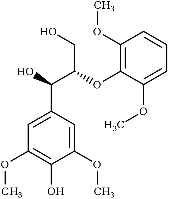
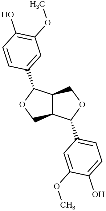
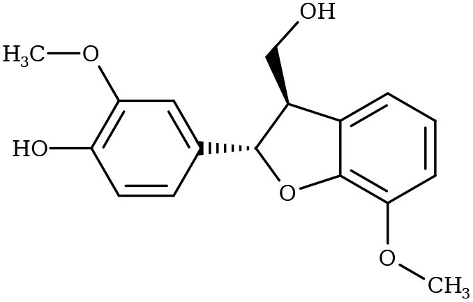
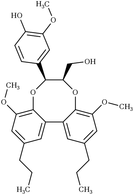
Creating models at that level of detail depends on an accurate description of atomic-scale interactions. This can be achieved by employing a classical approximation of the underlying quantum mechanical potential energy surface, otherwise known as a force field.³⁹ Previously, such an approximation was created for the three common lignin monomers and the most common lignin units (described by their characteristic interunit linkages).³⁸ Since that time, the force field was expanded by using a general force field (CGenFF)⁴⁰ to incorporate new linkages as the models demanded. However, these parameters taken by analogy from other similar biomolecules are known to be suboptimal, and reparameterization was warranted based on the internal quality metrics CGenFF produces.^41,42 Here, we systematically reparameterize the force field to put all lignin linkages and lignin modifications within a self-consistent framework, including linkages to carbohydrates, using parameters derived from CGenFF as a starting point (Fig. 1). Through combination of these constituent elements, true native-like lignin structures and lignin degradation products can be modeled, as demonstrated in Fig. S1.†

Fig. 1 Chemical structures of all lignin monomers and linkages considered in this study, which expands on the three monomers and common linkages explicitly parameterized in the previous force field.³⁸ We emphasize that some of the chemistries displayed here are not observed in native lignin, but are used to populate appropriate stereochemistries in combined structures, such as in dibenzodioxocin structures demonstrated in Fig. S1,† or are common degradation products. Compounds were included based on a broader suite of known lignin linkages. To aid in subsequent discussion, the ring carbons of the guaiacyl monomer have additionally been numbered as they are used consistently throughout the forcefield. Greek-letter based nomenclature for lignin linkages is used throughout.

The reparameterization follows the standard CHARMM parameterization methodology, with water interactions used to determine charges and bonded terms optimized against relaxed potential energy scans of internal molecular degrees of freedom.^40–44 Since this optimization incorporates target data from all target molecules simultaneously, the charge optimization uses a grouping scheme to create transferable charge groups that are consistent across all lignins. In addition, a new GPU-accelerated evaluation of the bonded objective function was implemented to make the bonded optimization tractable.

The result of this effort is a force field that reproduces the geometries and energies from quantum mechanical calculations more accurately than the generalized CGenFF parameter set. This includes an average 0.2 kcal mol⁻¹ reduction in the mean squared error of the water interaction energies, improved vaporization enthalpies, as well as significant reductions in the energy residuals along a potential energy surface. These improvements in energy do not increase geometrical deviation from quantum mechanical minima, and in fact improve specific features within aqueous and crystalline lignin simulation that were not well reproduced in previous general force fields. These improvements represent a significant advance overall in lignin simulations, enabling direct simulation of most lignin topologies under a unified framework.

2. Parameterization theory

The typical point-charge additive classical molecular mechanics force field for small molecules in a condensed phase, such as GROMOS,^45,46 OPLS,^47,48 AMBER^49,50 or CHARMM,^40,43,51 decomposes energy terms for a particular molecular pose into two parts; non-bonded and a bonded components, as described in eqn (1) for the CHARMM force field.^43,51

This energy function includes well known physical constants, geometrical measurements, and harmonic or sinusoidal approximations built-in to classical molecular mechanics models. However, the terms within eqn (1) highlighted by circles or squares are free parameters that must be determined to describe the energetics of molecular poses. The creation of a classical molecular mechanics force field requires a collection of target data, and adjustment of the free parameters such that the parameters chosen reproduce the target data. As the different force fields have different philosophies on what target data to optimize against, and specific adjustments were made to account for the branched structure of lignin, the ESI† provides additional details about the overall parameterization procedure in CHARMM,^40,44 and how it compares with force fields for other biopolymers.^52–56 The extended ESI† discussion also details the features required for our lignin parameterization workflow that are missing in existing parameterization tools such as the force field toolkit (ffTK),⁴⁴ ForceBalance,⁵⁷ the Visual Force Field Derivation Toolkit (VFFDT),⁵⁸ ForceFit,⁵⁹ or the general automated atomic model parameterization (GAAMP).⁶⁰

3. Methods

A series of python scripts were written to implement the overall workflow detailed in the ESI† to optimize the initial parameters determined from CGenFF⁴⁰ for the test compounds shown in Fig. 1. Largely, these python scripts reimplement the methodologies within ffTK⁴⁴ in a way that the objective functions within the charge and bonded optimizations can incorporate target data from several molecules simultaneously, which was not required for the small molecules ffTK was originally designed for. The greatest protocol deviations from standard approaches come in the bonded term optimization, where additional experimentation determined that unrestrained optimization leads to poor behavior during simulation. This finding lead to experimentation in charge assignment and in the limitations placed upon the optimizer during bonded term optimization, which is detailed primarily in the ESI.† Note that we refit only the circled terms from eqn (1), taking the non-bonded Lennard-Jones terms directly by analogy from CGenFF as has been recommended previously,⁴⁴ and eliminating the few improper terms originally found in the CGenFF description of lignin, which are unnecessary to recapitulate the structure and energetics of lignin.

3.1. Test compounds and initial parameter generation

The lignin test compounds (Fig. 1), were chosen by considering a combination of literature sources highlighting specific lignin chemistries with practical considerations regarding the construction of target data. Monomeric units are the simplest, with three chemistries predominating in natural lignins,^5,21 although we also include caffeyl-lignin^16,61,62 due to its discovery in seed coats⁶¹ (Fig. 1, Monomers). Tricin, while strictly speaking a flavonoid rather than a typical lignin monomer, is also parameterized, due to its role in monocot lignin biosynthesis.^63,64 The small size of the monomers makes quantum mechanical calculations inexpensive, which allows us to also construct target data for the observed variations of these monomers at the C1 position⁶⁵ (Fig. 1, End Caps), effectively covering the full space of observed monomeric lignins. As the quantum methods CHARMM parameterization demands scale polynomially (N⁵) with the number of atoms,⁶⁶ only lignin dimers^{20,65,67–69} were explicitly parameterized (Fig. 1, Lignin Linkages) in addition to the aforementioned monomers. Trimer-scale linkages, e.g., spirodienone,⁶⁸ are not included, as the increased size of the test compounds make the creation of target data impractical. For studies of these larger, rarer linkages, our parameterization experience suggests that a general force field would be a reasonable starting point for these systems.

Dimers in which lignin is linked to a carbohydrate are also new with this force field (Fig. 1, Carbohydrate Linkages). Although these sugar linkages are only explicitly parameterized for five membered rings such as those found in arabinose, the modular nature of the carbohydrate force field^70,71 makes creating the appropriate patches for a six membered ring a straightforward exercise in renaming the appropriate atom types, and are included in the topology files provided in the ESI.† Strong experimental evidence shows that lignin links to hemicellulose via ferulate esters, which may themselves be linked together in ways not seen in general lignin linkages.^68,69,72 These 8,8-diferulate linkages are highly charged at neutral pH, which can cause problems during parameterization in the convergence of compound–water interaction calculations, so these are treated as being protonated. Other evidence shows alternative linkage topologies may also be possible, although the nomenclature is less well established.⁶⁸

Natural lignin is a racemic mixture,^73,74 rather than demonstrating uniform chirality as in other biological polymers such as proteins or DNA.⁷⁵ To account for this, molecular geometries were optimized at a MP2/6-31G* level of theory using Gaussian 09 ^76,77 for every possible stereochemical combination of lignin within every compound shown in Fig. 1. This resulted in 199 total optimized geometries at quantum mechanical minima, which are used as the starting points for subsequent calculations within the charge optimization and bonded optimization steps.

For each compound, initial atom typing and parameter determination was carried out through the ParamChem web interface to CGenFF.⁴⁰ Attempts to split atom types based on the local geometry around each atom were not found to significantly improve the overall quality of the parameters, and so the CGenFF atom types are largely retained. However, aromatic ring carbon atoms with the original CGenFF type CG2R61 were split based on the ring substituents, where aromatic carbons bonded to methoxy groups or alcohols are given their own type (Fig. 2). To distinguish the new atom types from those found in CGenFF, new parameters found in the ESI† insert an “L” into the second position of the atom type. Thus CG2R61 becomes the CLG2R61 type, which was split further into CLG2R6A if bonded to a hydroxyl group, or CLG2R6B if bonded to another oxygen, such as in a methoxy group or ether. These new atom types inherit the Lennard-Jones parameters from the progenitor CGenFF atom type.

Fig. 2 Example of how compounds, in this case coniferyl alcohol and caffeyl alcohol (left), are translated into the graphs used for both neighborhood-based and group-based charge equivalence determinations. In these graphs, the nodes are labeled according to atomic index, and the edges show the bonding topology. The atom typing graphs (middle) are colored according to atom type, where atoms with equivalent atom types are represented by circles of the same color. Thus for coniferyl alcohol, atoms 16 and 18, the carbons of the –ene group, are colored the same, and also share a color with the equivalent carbons in caffeyl alcohol, as well as with any other similar functional groups throughout the test compound set. This also demonstrates the split of the CG2R61 type (orange), which was assigned by CGenFF to be the atom type within most aromatic rings. We create new atom types, colored here in darker and lighter purple, to split from CG2R61 when it is bonded to oxygen-containing compounds. The group assignment (right) coloration is different, in that unique colors only denote individual “groups” (atoms whose charge should sum to an integer) within each molecule. If the subgraphs formed by each group are identical (e.g. atoms 4, 5, and 6 and atoms 7, 8, and 9 within caffeyl alcohol), the group-based charge optimization assigns the same charges on equivalent atoms. More examples of conversion between chemical structure and near-integer sum groups are presented in Fig. S2.†

3.2. Charge & bond optimization

As stated previously, the optimization process inherits its approach from standard tools to determine CHARMM parameters, as laid out in prior literature.^40,44,78 However, the result of the optimization does depend on the implementation, and thus we experimented with different ways of assigning equivalent charges, dihedral torsion limits, and the incorporation of force information into the force field. Extended discussion of the methods and their implementation can be found in the ESI,† but the noteworthy features are listed here for completeness.

1. Two alternative charge group definitions, neighbor-based and group-based (Fig. 2 & S2†). Both use subgraph isomorphism⁷⁹ to determine equivalent atoms.

2. Water interactions computed at the HF/6-31G* level of theory.⁸⁰

3. Optimization of bonded and nonbonded objective functions (eqn (S1) and (S2)†) with the L-BFGS-B algorithm.⁸¹

4. Structural perturbations to compute bond, angle, and dihedral scans carried out at the MP2/6-31G* level of theory.⁷⁷

5. Four different approaches to restricting allowed values in the dihedral term Fourier series (Table S1†), reducible to a linear least-squares problem.⁸²

6. Thrust⁸³ and CUDA⁸⁴ libraries were used to accelerate evaluation of the bonded objective function.

7. Incorporation of force magnitudes at quantum minima into the minimized objective function (eqn (S2)†) through a weighting parameter v.

3.3. Analysis

Upon completion of the optimization procedure under the different implementation conditions tested, analysis was performed via a number of tests. These tests compared the fitted parameters to both the target data used to generate the fit and simulation observables that were not included during the optimization process. The charges were evaluated based on how well they recapitulated the interaction energies used as target data, as well as the scale of the adjustments made relative to the CGenFF starting point and computed enthalpy of vaporization for a subset of molecules for which experimental data are available. Likewise, the bonded terms were evaluated with respect to how small the residuals were relative to the available target data. Separately, we analyzed force magnitudes at the quantum mechanical minimum energy geometries to determine the degree of overfitting in constructing the molecular mechanics energy landscape.

In addition to target data comparisons, the bonded terms were also evaluated in terms of how far, in geometric space, minimized structures in the newly optimized force field diverged from previously calculated quantum mechanical optimized structures. The classical minimization was carried out in NAMD 2.12⁸⁵ using the 16 different parameter combinations (4 dihedral sets, 4 different values for v in eqn (S2)†) starting from each of the 199 minimum energy configurations determined quantum mechanically. This is a surrogate metric for overall force field accuracy, as our optimization scheme does not guarantee that the minimum energy configurations determined from quantum level calculations are minimum energy points on the potential energy landscape created by our classical force field (Fig. S3†). On the multidimensional potential energy surface, if there is a net force along these degrees of freedom orthogonal to the quantum mechanical target data scans, the resulting geometry will distort. Minimizing the structures with this new classical potential energy surface informs us as to how influential these orthogonal degrees of freedom would be in typical simulation systems; we used the root mean square deviation (RMSD) between the classical and quantum minimum energy structures as a proxy for overfitting in the optimization.

Beyond minimization, a set of simulations were carried out to determine the enthalpy of vaporization both from the initial CGenFF parameter set as well as the newly optimized set. Due to the paucity of available reference data, these calculations were only carried out for phenol, catechol, guaiacol, and syringol. The enthalpy of vaporization (ΔH_vap) can be estimated from the average potential energies from molecular dynamics trajectories in gas and liquid phases ΔH_vap = U_g − U_l + kT, where U_g and U_l are the average molecular potential energies in gas and liquid phases, respectively, observed during simulation.⁸⁶ Thus, each of the compounds were simulated four times, once with CGenFF parameters in the gas phase, once with CGenFF parameters in the liquid phase, and in gas and liquid phases with our newly optimized parameters instead. These 2 ns simulations were carried out in NAMD 2.12 (ref. 85) with 2 fs timesteps and maintained at 298 K through the use of a Langevin thermostat.⁸⁷ To achieve a liquid rather than a crystalline phase, 500 copies of each compound were put into a box with 60 Å sides using the insert-molecules program from the GROMACS simulation suite,⁸⁸ and pressure was maintained at 1 atm via the Langevin piston method.⁸⁹ After 0.4 ns for simulation box equilibration, the last 1.6 ns of simulation were used in the calculation of ΔH_vap.

Another comparison to experimental observables comes in the form of crystal simulations. Existing lignin-related compound crystal structures are present in the Cambridge Structural Database.⁹⁰ We took a set of 20 of these structures (8 monomeric crystals,^91–96 11 dimeric crystals,^97–106,108 and a trimeric crystal¹⁰⁷), and simulate them for 20 ns with both the general CGenFF and the newly developed lignin force field. Chimera¹⁰⁹ was used to create a complete unit cell model of each molecule, which was then replicated along each axis using the VMD¹¹⁰ plugin TopoTools such that the minimum dimension of the crystal was at least 50 Å. The simulation was performed using GROMACS 2016.4,^88,111 using TopoGromacs¹¹² to facilitate the conversion between input formats. The simulation thermostat was set to the temperature at which the crystal structure was obtained (Tables 1 and 2) using a Nose–Hoover thermostat.¹¹³ Other simulation parameters were identical across crystals. Long-range electrostatics was handled using particle mesh Ewald¹¹⁴ with a 1.2 Å grid spacing past the typical 12 Å short-range cutoff and 10 Å switching distance. Bonds to hydrogen were constrained using P-LINCS,¹¹⁵ enabling a 2 fs integration timestep. To allow the triclinic unit cell vectors to change independently, an anisotropic Berendsen barostat¹¹⁶ was used to maintain the pressure at 1 atm. The last 10 ns of simulation was consistently used when measuring changes in crystal structure and density, as well as molecular-level changes in structure.

Table 1 Summary of monomeric lignin-crystals simulated. This includes the small molecule structure, the common name of the molecule, the Cambridge Structural Database⁹⁰ code, and the temperature T at which the underlying X-ray data were collected. Dimeric and trimeric lignin structures are presented in Table 2

Structure	Name	CSD code	T (K)
	Catechol	CATCOL13	100
	p-Hydroxybenzaldehyde	PHBALD11 ^91	296
	Vanillin	YUHTEA01	123
	Vanillin	YUHTEA03 ^92	296
	Syringaldehyde	IZALAW^93	293
	Coniferaldehyde	SIPKEH^94	295
	Vanillic acid	CEHGUS^95	293
	Ferulic acid	GASVOL01 ^96	110

---

Table 2 Summary of multimeric lignin-crystals simulated, with the small molecule structure, coupling shorthand, Cambridge Structural Database⁹⁰ code, and temperature T at which the underlying X-ray data were collected. The linkage shorthand used here refers to the monomers and linkages (Fig. 1) used to construct each structure, and does not distinguish between end-caps that were applied to individual monomers. The dibenzodioxocin-like structure is not labeled in this way, and instead is the combination of three guaiacyl monomers, linked together by α-O-4, β-O-4, and 5-5 linkages

Structure	Shorthand	CSD code	T (K)	Structure	Shorthand	CSD code	T (K)
	G-βO4-G	RABWUM^97	153		G-βO4-G	SIPPEM^98	295
	S-βO4-G	VADDOT^99	295		S-βO4-S	SAZHEG^100	295
	S-βO4-S	FOCGUA^101	173		S-βO4-S	IDIKIP^102	183
	G-ββ-G	INELIW^103	153		G-ββ -G	INELIW01^104	153
	G-ββ-G	FAFXUF^105	295		G-β5-G	FUMVUE^106	295
	Dibenzodioxocin	TUGWAT^107	193		G-55-G	UJOGIK^108	153

---

Like much of the parameterization framework, the analysis leveraged several python libraries, including NumPy,¹¹⁷ SciPy, matplotlib,¹¹⁸ NetworkX,¹¹⁹ as well as VMD for visualization.¹¹⁰ To generate 2-D representations of each molecule, we extensively used Marvin and its molconvert tool, developed by ChemAxon (https://www.chemaxon.com).

4. Results and discussion

Having reimplemented the typical CHARMM parameterization workflow, there were a number of implementation questions that needed to be evaluated. These questions include which atoms should carry the same atomic point charges across different molecules to aid in parameter transferability, and what are the most appropriate dihedral terms to include to accurately recapitulate the potential energy surface. As mentioned in the Methods, we tried two separate approaches to determining equivalent chemical environments for atomic charges, as well as four variations for both the dihedral set and the incorporation of force data into the optimization (eqn (S2)†). Determining which of the possible approaches is most suitable overall is discussed thoroughly in the ESI,† where quantitative metrics were evaluated to determine the optimal parameter set, also provided in the ESI.† The results presented here only compare the optimal parameter set to the original CGenFF starting point, highlighting the improvements obtained relative to a generic force field.

4.1. Charge analysis

As our charge optimization objective function (eqn (S1)†) explicitly considers lignin–water interaction energies as a metric to improve, we expected improvement in matching quantum-mechanical interaction energies with the newly optimized force field (Fig. 3). The interaction energy matching between quantum and molecular mechanical reduced the scattering within Fig. 3A compared to the CGenFF starting point, with most interaction energies improving. The improvement in practical terms is demonstrated in Fig. 3B, where we see that, after optimization, approximately 50% of the calculated water interaction energies are within 0.5 kcal mol⁻¹ of their quantum energy targets, a significant improvement on the 40% from the CGenFF starting point. These improvements are most striking at the tail end of the distributions, with residual range spanning the 10th and 90th percentiles shrinking to just over 1 kcal mol⁻¹, rather than the 1.3 kcal mol⁻¹ as in CGenFF.

Fig. 3 Comparison of water interaction energies determined through quantum calculations and the parameterized point charges in our molecular mechanics framework. (A) Scatter diagram comparing the adjusted quantum (QM) and classical (MM) interaction energies for the low interaction energy poses (E^int_QM < 5 kcal mol⁻¹ and E^int_VDW < 1 kcal mol⁻¹) for CGenFF (black) and our optimized lignin force field (violet). The cutoffs reduce the number of points plotted, which improves the visual clarity. The solid black diagonal line indicates the line where E^int_QM = E^int_MM, which is surrounded by darker and lighter bands indicating deviations of 1 kcal mol⁻¹ and 2 kcal mol⁻¹. In (B), the scatter plot is transformed into a cumulative distribution of the interaction energy residuals (E^int_QM − E^int_MM), with a highlighted grey region representing residuals less than 0.5 kcal mol⁻¹.

These improvements in interaction energy generally required only small changes from the initial point charges provided by CGenFF. The charge changes were bounded by the imposed constraints during the optimization process, in which a maximum change of 0.25 charge units was allowed. This upper bound is almost never reached, with most atomic charge changes being restricted to less than 0.05 charge units (Fig. 4 and Table S2†). The charge changes observed depend on the identity of the atom. Most hydrogen charges were unchanged, with much of the remainder changing by less than 0.02 charge units to reflect the modifications required to make charge groups integer charges. Oxygen atoms, by contrast, tend to show the largest charge changes, with many charges becoming more positive through optimization, counterbalanced by small decreases in carbon charges. In effect, we have lowered the polarization of individual functional groups relative to the starting point. The CHARMM fixed-charge force field is intentionally over polarized to better reproduce structure and energetics in the condensed phase,^70,120 which we accounted for by biasing the molecular dipole to be between 20–50% larger in our parameter set than the quantum dipoles in a vacuum, consistent with CHARMM parameterization methodology.^40,44

Fig. 4 Cumulative distribution of the difference in charges between the initial charges assigned by CGenFF (q_CGenFF) and the new charges assigned through the near-integer sum grouping method implemented here (q_opt). This includes breaking down the difference in charge depending on the element of each atom, since most hydrogen charges were explicitly held fixed to values found elsewhere in the CHARMM force field. Most other charges change only modestly, and very few drift as much as they were allowed by the imposed bounds in the optimization. An alternative quantification including the neighbor-based charges is presented in Table S2.†

A quantitative point of comparison to assess the impact of polarization is to compute an enthalpy of vaporization,^70,120 a quantity dependent on the quality of the non-bonded parameters. As evidenced in Table 3, our newly optimized charges yielded enthalpies of vaporization that were uniformly closer to the available experimental reference values,^121–123 as is particularly noticeable when a methoxy group is present (as in guaiacol or syringol). One possible explanation is that the adjacent alcohol to the methoxy group in lignin withdraws electrons more strongly relative to the methoxy groups, reducing the polarization of the methoxy groups in native lignin. However, the parameterized molecule from CGenFF that is used for methoxy charge assignment, anisole, has an isolated methoxy. The isolation of this electron withdrawing oxygen increases the magnitude of the partial negative charge, overpolarizing guaiacol and syringol in CGenFF and leading to less accurate vaporization enthalpies (Table 3). This suggests that the reduced polarization of individual functional groups while retaining the overall polarization of the whole molecule is an improvement on the CGenFF defaults, although the conclusion is limited by the availability of comparable reference data. However, given the evidence showing the improvement of the new charge set relative to the initial charges provided by CGenFF in recapitulating lignin–water interactions (Fig. 3 and Table S3†), we think that the improvement is not isolated to just the small organic molecules tested in Table 3, but that the new model more accurately tracks experimental observables more broadly.

Table 3 Enthalpy of vaporization (ΔH_vap, reported in kJ mol⁻¹) for small organic molecules constructed with this parameter set and CGenFF compared to existing experimental data

Compound	Literature ΔHvap	CGenFF ΔHvap	Opt. ΔHvap
a For syringol, a heat of vaporization is not available, and a heat of sublimation is used as the reference state instead. Based on the difference between heats of sublimation and vaporization for catechol,^121 the heat of vaporization for syringol is likely 20–30 lower than this literature value for sublimation.
Phenol	59.1 (ref. 122)	62.1 ± 1.2	60.1 ± 0.9
Catechol	70.0 ± 0.7 (ref. 121)	64.3 ± 1.1	68.9 ± 1.1
Guaiacol	62.6 ± 0.5 (ref. 123)	46.0 ± 1.3	59.5 ± 1.3
Syringol	98.4 ± 1.1^a (ref. 123)	53.1 ± 1.3	67.3 ± 1.4

---

4.2. Intramolecular interactions

As described in the ESI,† 16 different bonded optimizations were tested during the optimization of the bonded terms of the potential energy function (eqn (1)). Relaxed quantum mechanical geometry optimizations that scan along internal degrees of freedom were the primary input for this optimization, with a selection of these scan results shown in Fig. 5.

Fig. 5 Examples of the quantum mechanical and classical potential energy surface for a limited subset of the 2574 bond, angle or dihedral scans used as target data. Each subpanel shows the energy trace for a series of molecular poses corresponding to a relaxed quantum mechanical energy scan along a specific degree of freedom. The quantum mechanical energy trace is drawn in black, the CGenFF energy trace is gray, and the energy trace after optimization is shown in orange, matching the color scheme used for the multi-set optimization shown in Fig. S4.† A molecular image of the compound being scanned in its central pose can be found within each panel, with a black arrow indicating which degree of freedom is being probed by the scan. (A) Shows a typical methoxy rotation, (B) demonstrates an angular change between a lignin and sugar monomer, (C) shows an α-hydroxyl rotation, and (D) shows a rotation around an ester-adjacent bond. A similar figure showing the scans for the alternative dihedral sets is presented as Fig. S4.†

Subpanels within Fig. 5 highlight general trends within the larger population of potential energy scans. Sometimes, as in Fig. 5A, CGenFF did not have the right weighting between multiplicities to fully recapitulate the underlying quantum mechanical potential energy scan. Another related example is presented in Fig. 5B, where the optimum angle at the bridging oxygen was not originally correct in CGenFF due to poor analogy, but is improved in our optimization. In other cases, the improvements relative to CGenFF were modest, such as in Fig. 5C and D, where the quantum potential energy surface is not perfectly fit by the optimized parameter set. The residuals relative to quantum, although generally smaller than in CGenFF, were on the order of 1 kcal mol⁻¹. Forcing the residuals to zero appears to be impossible given the structure of eqn (1), as even when all dihedral terms in the Fourier sum were nonzero, the overall energy trends were not always preserved (Fig. S4E & S4F†).

Broader analysis showed significant reductions in the quantum mechanical energy residuals from CGenFF to the newly optimized parameters (Table S4†), as the Cauchy distribution of residuals (Fig. S5†) showed significantly less spread away from the mean of zero after optimization. Ideally the distribution would have zero width, with all molecular mechanics energies coincident with quantum energies, but the harmonic and sinusoidal approximations made in the potential energy function (eqn (1)) limit the eventual accuracy of the force field. Typical errors in local potential energy minima were around 0.2 kcal mol⁻¹, with larger errors sometimes exceeding 1 kcal mol⁻¹ for barrier heights (Fig. 5 & S32†). The improved energies also improve local molecular structure, such as when comparing RMSDs relative to a quantum minimized structure (Fig. S6 & S7†).

4.3. Structure analysis

Due to the heterogeneity of native lignin polymers, few experiments exist with which the overall performance of the force field can be directly compared. Small molecule crystal structures of lignin derived compounds (Tables 1 and 2) provide a starting point for lignin structural studies. By comparing the published crystal structures with the results of simulation using both our developed optimized force field and a general CGenFF force field (Table 4 and Fig. S8–S27†), we assess the improvements in structure along a number of metrics. In 14 of the 20 crystals simulated, the optimized lignin force field had a density closer to the crystalline density than did the CGenFF force field. In three quarters of the simulated crystals, the RMSD of the whole crystal (RMSD^C) is improved relative to the experimental starting structure, once by nearly 3 Å when CGenFF parameters caused the crystal to melt. By contrast, the RMSD difference when CGenFF better matched the crystal tend to be small. The exceptions were syringaldehyde and the G-55-G crystals, in which both the new force field and CGenFF adopt a new crystal packing during simulation as judged by the unit cell parameters (Table S5†), increasing deviations from the initial crystal structure. Together, these results highlight the improvement in the intermolecular interactions in the optimized force field and the resulting improvement in quantifiable experimental observables.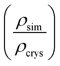

Table 4 Comparison of mean crystal properties when simulated using the developed force field (Opt), and using the general force field (CGenFF). This includes the density (ρ) ratio of simulated and experimental crystals , the RMSD of the complete simulated crystal relative to the starting crystallographic structure (RMSD^C), and the average intramolecular RMSD for individual molecules within the crystal (RMSD^M). The uncertainties in the last digit are reported in parentheses, and were determined from the standard deviation of the 200 samples taken over the last 10 ns of the source trajectory used to determine the mean. The separator between ferulic acid and G-βO4-G marks the boundary between the monomeric crystals (Table 1) and multimeric crystals (Table 2)

Name/shorthand	CSD code	ρ Opt ratio	ρ CGenFF ratio	RMSD^COpt (Å)	RMSD^CCGenFF (Å)	RMSD^MOpt (Å)	RMSD^MCGenFF (Å)
Catechol	CATCOL13	0.9687(2)	0.9708(2)	0.977(8)	1.336(8)	0.05(1)	0.07(2)
p-Hydroxybenzaldehyde	PHBALD11	0.9755(6)	0.9607(6)	1.09(2)	1.26(2)	0.11(3)	0.11(3)
Vanillin	YUHTEA01	0.9749(2)	0.9571(2)	1.331(8)	1.426(9)	0.10(2)	0.09(2)
Vanillin	YUHTEA03	1.061(1)	1.0451(4)	1.52(3)	1.61(1)	0.14(4)	0.13(3)
Syringaldehyde	IZALAW	0.9491(4)	0.9214(3)	8.92(1)	8.40(1)	0.19(4)	0.18(4)
Coniferaldehyde	SIPKEH	0.9913(6)	0.9867(5)	3.16(2)	3.14(2)	0.5(1)	0.3(1)
Vanillic acid	CEHGUS	0.9360(4)	0.9348(5)	1.01(1)	1.06(1)	0.15(4)	0.15(4)
Ferulic acid	GASVOL01	0.9557(2)	0.9468(2)	0.837(6)	1.352(7)	0.11(3)	0.13(4)
G-βO4-G	RABWUM	0.9630(2)	0.9584(2)	0.592(7)	0.631(6)	0.20(4)	0.16(4)
G-βO4-G	SIPPEM	0.9538(3)	0.9543(3)	0.93(1)	1.100(9)	0.36(9)	0.38(5)
S-βO4-G	VADDOT	0.9546(3)	0.9451(4)	1.15(1)	1.72(2)	0.29(7)	0.30(7)
S-βO4-S	SAZHEG	0.9474(4)	0.9475(4)	0.95(1)	0.84(1)	0.25(6)	0.27(9)
S-βO4-S	FOCGUA	0.9559(1)	0.9393(2)	0.917(7)	0.84(1)	0.19(4)	0.17(4)
S-βO4-S	IDIKIP	0.9480(2)	0.9289(3)	0.84(1)	1.83(1)	0.19(4)	0.23(6)
G-ββ-G	INELIW	0.9626(2)	0.9460(3)	0.786(9)	1.42(1)	0.11(7)	0.11(7)
G-ββ-G	INELIW01	0.9656(2)	0.9543(2)	0.82(2)	2.322(8)	0.12(9)	0.2(2)
G-ββ-G	FAFXUF	0.9368(4)	0.8415(8)	0.99(1)	3.97(2)	0.19(4)	1.5(3)
G-β5-G	FUMVUE	0.9357(3)	0.9367(3)	1.01(1)	1.07(1)	0.25(7)	0.23(6)
Dibenzodioxocin	TUGWAT	0.9518(4)	0.9603(3)	0.88(2)	1.23(2)	0.29(4)	0.26(9)
G-55-G	UJOGIK	0.9692(1)	0.9482(4)	2.521(4)	1.77(4)	0.78(4)	0.6(2)

---

The improvements in crystalline behavior were not the result of intramolecular interactions, as the average structural change observed within individual molecules (RMSD^M) was typically small, the expected result for a thermalized crystal (Fig. S8–S27†). Within molecules, the mean differences in RMSD^M were typically less than 0.04 Å between CGenFF and optimized force fields (Table 4). Of the remaining four molecules with significant differences in RMSD^M, the two force fields are evenly split in performance, with two exhibiting a lower RMSD in CGenFF and two instead showing smaller deviations from the crystal under the optimized force field, although again CGenFF occasionally exhibited much higher RMSDs than is seen in the reverse direction. The high RMSDs for specific molecules are emblematic of the trends shown in Fig. 5. Usually, CGenFF parameters adequately described the underlying potential energy surface of the molecule, resulting in comparable RMSD^M values with the newly optimized force field. However, there are internal degrees of freedom that are poorly described by a generic force field, such as in Fig. 5C & D, which can dramatically increase the RMSD^M. In particular, the description of the bonds and angles within a β–β linkage improved significantly in the new force field, reducing the molecular RMSD^M for these lignin linkages.

Given the good structural agreement between experiment and simulation, we need to consider the possibility of our parameter set being overfit given the target data provided during optimization. The minimal structural deviations observed for our parameterized compounds against quantum-derived optimum structures (Fig. S6 and Table S6†) suggested that the optimum geometries coincide. Additional tests of our force field compared against small molecule crystal structures also indicated that the molecular geometries were in line with a typical all-atom force field (Table 4). This analysis suggests that the overfitting scenario sketched out in Fig. S3† was avoided in force field development. We conclude that the developed force field for lignin should be applicable to general lignin polymers.

5. Conclusion

The parameter set generated here is an important step forward towards accurate molecular simulation of lignin. These new lignin parameters are self-consistent, and extend the prior force field³⁸ into linkage types that were not previously parameterized. As we purposefully chose charge and parameter sets that are local to simplify lignin polymer construction, it is straightforward to apply these parameters to newly built lignin systems. In addition, strict adherence to the CHARMM parameterization philosophy maximizes the compatibility between the lignin parameters determined here and the rest of the CHARMM force field. Furthermore, with specifically parameterized linkages to sugars, this new force field enables the construction of complete biomass models, including direct interaction between lignin and hemicellulose, thereby permitting new questions of biomass structure and interaction to be addressed through computational modeling.

The extensive parameterization carried out here offers a number of improvements over a general force field. The new parameters better recapitulated experimental enthalpy of vaporizations (Table 3), improved the fit against the scanned potential energy surfaces (Fig. 5), and better mimicked structures seen in small crystals of lignin analogs (Table 4). These improvements came with only minimally increasing the number of free parameters relative to the original general force field, specifically splitting up aromatic carbon parameters depending on the bonded functional groups to reproduce the different angles seen in minimum energy structures (Fig. S28†), and adding selected dihedral terms to fit specific potential energy scans (Fig. S4A and S4B†). The improved energetics did not come at the cost of structure, with minimum energy configurations that differed from quantum calculations just as was observed for the general force field (Table S6†), suggesting that the parameters are not overfitted to the target data, and should be broadly applicable to native lignins.

There are innovations in the parameterization process that can be applied to other systems. The GPU-accelerated bonded optimization procedure is generically useful to any parameterization effort of classical force fields, allowing a quick assessment of how each term contributes to the overall quality of the optimized parameters, and how individual parameters should change to improve the global fit. Our attempts to include force information into the bonded optimization process ultimately did not improve the energetics or structure of the generated parameter set. However, with the machinery now in place to include that as part of the objective function and within the optimization workflow, we are confident that in the future others can incorporate forces into their own workflows and possibly eliminate the time-consuming potential energy scans.

It is also eminently possible that emerging generic force fields based on machine learning^124–126 will obviate the need for force fields tailored to specific biopolymers in the future. However, for current ongoing work in modeling lignin within biological or industrial processes, the force field as it stands now significantly expands the set of currently tractable problems, including those featuring complex lignin topologies and interactions between lignin and hemicelluloses that were not explicitly parameterized previously. We envision tools that work in conjunction with this force field to facilitate lignin atomic model construction and enable researchers to visualize their molecules of interest.

Conflicts of interest

There are no conflicts to declare.

Acknowledgements

We thank Tom Elder for fruitful discussions on what lignin topologies should be parameterized. This work was authored in part by Alliance for Sustainable Energy, LLC, the manager and operator of the National Renewable Energy Laboratory for the U.S. Department of Energy (DOE) under Contract No. DE-AC36-08GO28308. JVV acknowledges support by the NREL Director's Fellowship funded by the Laboratory Directed Research and Development (LDRD) program. JVV, MFC, and GTB acknowledge funding from the U.S. Department of Energy Office of Energy Efficiency and Renewable Energy Bioenergy Technology Office. GTB acknowledges funding from the Center for Bioenergy Innovation, which is a U.S. DOE Bioenergy Research Center supported by the Office of Biological and Environmental Research in the DOE Office of Science. LP was supported by the U.S. Department of Energy Genomic Science Program, Office of Biological and Environmental Research, U. S. Department of Energy, under Contract FWP ERKP752. JR was funded by the DOE Great Lakes Bioenergy Research Center (DOE Office of Science DE-SC0018409). A portion of the research was performed using computational resources sponsored by the Department of Energy's Office of Energy Efficiency and Renewable Energy and located at the National Renewable Energy Laboratory. This work used the Extreme Science and Engineering Discovery Environment (XSEDE)¹²⁷ through grant TG-MCB090159 to GTB, specifically the Stampede2 system at the University of Texas at Austin in the Texas Advanced Computing Center. The views expressed in the article do not necessarily represent the views of the DOE or the U.S. Government.

References

1. C. Beer, M. Reichstein, E. Tomelleri, P. Ciais, M. Jung, N. Carvalhais, C. Rodenbeck, M. A. Arain, D. Baldocchi, G. B. Bonan, A. Bondeau, A. Cescatti, G. Lasslop, A. Lindroth, M. Lomas, S. Luyssaert, H. Margolis, K. W. Oleson, O. Roupsard, E. Veenendaal, N. Viovy, C. Williams, F. I. Woodward and D. Papale, Science, 2010, 329, 834–838.
2. J. E. Campbell, J. A. Berry, U. Seibt, S. J. Smith, S. A. Montzka, T. Launois, S. Belviso, L. Bopp and M. Laine, Nature, 2017, 544, 84–87.
3. M. Pauly and K. Keegstra, Plant J., 2008, 54, 559–568.
4. A. J. Ragauskas, G. T. Beckham, M. J. Biddy, R. Chandra, F. Chen, M. F. Davis, B. H. Davison, R. A. Dixon, P. Gilna, M. Keller, P. Langan, A. K. Naskar, J. N. Saddler, T. J. Tschaplinski, G. A. Tuskan and C. E. Wyman, Science, 2014, 344, 1246843–1246843.
5. W. Boerjan, J. Ralph and M. Baucher, Annu. Rev. Plant Biol., 2003, 54, 519–546.
6. N. D. Bonawitz, J. I. Kim, Y. Tobimatsu, P. N. Ciesielski, N. A. Anderson, E. Ximenes, J. Maeda, J. Ralph, B. S. Donohoe, M. Ladisch and C. Chapple, Nature, 2014, 509, 376–380.
7. J. Liu, J. I. Kim, J. C. Cusumano, C. Chapple, N. Venugopalan, R. F. Fischetti and L. Makowski, Biotechnol. Biofuels, 2016, 9, 126.
8. J. L. Rahikainen, J. D. Evans, S. Mikander, A. Kalliola, T. Puranen, T. Tamminen, K. Marjamaa and K. Kruus, Enzyme Microb. Technol., 2013, 53, 315–321.
9. D. Gao, C. Haarmeyer, V. Balan, T. A. Whitehead, B. E. Dale and S. P. Chundawat, Biotechnol. Biofuels, 2014, 7, 175.
10. L. Qin, W.-C. Li, L. Liu, J.-Q. Zhu, X. Li, B.-Z. Li and Y.-J. Yuan, Biotechnol. Biofuels, 2016, 9, 70.
11. M. Kellock, J. Rahikainen, K. Marjamaa and K. Kruus, Bioresour. Technol., 2017, 232, 183–191.
12. W. Wu, T. Dutta, A. M. Varman, A. Eudes, B. Manalansan, D. Loqué and S. Singh, Sci. Rep., 2017, 7, 8420.
13. Z. Sun, B. Fridrich, A. de Santi, S. Elangovan and K. Barta, Chem. Rev., 2018, 118, 614–678.
14. S. Barsberg, P. Matousek, M. Towrie, H. Jørgensen and C. Felby, Biophys. J., 2006, 90, 2978–2986.
15. A. K. Sangha, J. M. Parks, R. F. Standaert, A. Ziebell, M. Davis and J. C. Smith, J. Phys. Chem. B, 2012, 116, 4760–4768.
16. L. Berstis, T. Elder, M. Crowley and G. T. Beckham, ACS Sustainable Chem. Eng., 2016, 4, 5327–5335.
17. C. W. Johnson, D. Salvachúa, P. Khanna, H. Smith, D. J. Peterson and G. T. Beckham, Metab. Eng. Commun., 2016, 3, 111–119.
18. S. Wang, L. Shuai, B. Saha, D. G. Vlachos and T. H. Epps, ACS Cent. Sci., 2018, 4, 701–708.
19. A. J. Yanez, W. Li, R. Mabon and L. J. Broadbelt, Energy Fuels, 2016, 30, 5835–5845.
20. L. D. Dellon, A. J. Yanez, W. Li, R. Mabon and L. J. Broadbelt, Energy Fuels, 2017, 31, 8263–8274.
21. R. Vanholme, B. Demedts, K. Morreel, J. Ralph and W. Boerjan, Plant Physiol., 2010, 153, 895–905.
22. M. Konstantopoulou, P. J. Slator, C. R. Taylor, E. M. Wellington, G. Allison, A. L. Harper, I. Bancroft and T. D. Bugg, Nord. Pulp Pap. Res. J., 2017, 32, 493–507.
23. A. Lourenço, J. Rencoret, C. Chemetova, J. Gominho, A. Gutiérrez, J. C. del Río and H. Pereira, Front. Plant Sci., 2016, 7, 1612.
24. K. Fagerstedt, P. Saranpää, T. Tapanila, J. Immanen, J. Serra and K. Nieminen, Plants, 2015, 4, 183–195.
25. C. G. Yoo, A. Dumitrache, W. Muchero, J. Natzke, H. Akinosho, M. Li, R. W. Sykes, S. D. Brown, B. Davison, G. A. Tuskan, Y. Pu and A. J. Ragauskas, ACS Sustainable Chem. Eng., 2018, 6, 2162–2168.
26. E. Biazzi, N. Nazzicari, L. Pecetti, E. C. Brummer, A. Palmonari, A. Tava and P. Annicchiarico, PLoS One, 2017, 12, e0169234.
27. K. Morreel, O. Dima, H. Kim, F. Lu, C. Niculaes, R. Vanholme, R. Dauwe, G. Goeminne, D. Inze, E. Messens, J. Ralph and W. Boerjan, Plant Physiol., 2010, 153, 1464–1478.
28. G. van Erven, R. de Visser, D. W. H. Merkx, W. Strolenberg, P. de Gijsel, H. Gruppen and M. A. Kabel, Anal. Chem., 2017, 89, 10907–10916.
29. R. O. Dror, R. M. Dirks, J. Grossman, H. Xu and D. E. Shaw, Annu. Rev. Biophys., 2012, 41, 429–452.
30. H. I. Ingolfsson, C. Arnarez, X. Periole and S. J. Marrink, J. Cell Sci., 2016, 129, 257–268.
31. J. V. Vermaas, L. Petridis, X. Qi, R. Schulz, B. Lindner and J. C. Smith, Biotechnol. Biofuels, 2015, 8, 217.
32. A. K. Sangha, L. Petridis, J. C. Smith, A. Ziebell and J. M. Parks, Environ. Prog. Sustainable Energy, 2012, 31, 47–54.
33. J. Shi, K. Balamurugan, R. Parthasarathi, N. Sathitsuksanoh, S. Zhang, V. Stavila, V. Subramanian, B. A. Simmons and S. Singh, Green Chem., 2014, 16, 3830–3840.
34. M. D. Smith, B. Mostofian, X. Cheng, L. Petridis, C. M. Cai, C. E. Wyman and J. C. Smith, Green Chem., 2016, 18, 1268–1277.
35. M. D. Smith, X. Cheng, L. Petridis, B. Mostofian and J. C. Smith, Sci. Rep., 2017, 7, 14494.
36. C. Chen, L. Zhao, J. Wang and S. Lin, Ind. Eng. Chem. Res., 2017, 56, 12276–12288.
37. M. Li, Y. Pu and A. J. Ragauskas, Front. Chem., 2016, 4, 45.
38. L. Petridis and J. C. Smith, J. Comput. Chem., 2009, 30, 457–467.
39. L. Monticelli and D. P. Tieleman, in Biomolecular Simulations: Methods and Protocols, ed. L. Monticelli and E. Salonen, Humana Press, Totowa, NJ, 2013, ch. 8, pp. 197–213.
40. K. Vanommeslaeghe, E. Hatcher, C. Acharya, S. Kundu, S. Zhong, J. Shim, E. Darian, O. Guvench, P. Lopes, I. Vorobyov and A. D. Mackerell, J. Comput. Chem., 2010, 31, 671–690.
41. K. Vanommeslaeghe and A. D. MacKerell, J. Chem. Inf. Model., 2012, 52, 3144–3154.
42. K. Vanommeslaeghe, E. P. Raman and A. D. MacKerell, J. Chem. Inf. Model., 2012, 52, 3155–3168.
43. A. D. MacKerell, B. Brooks, C. L. Brooks, L. Nilsson, B. Roux, Y. Won and M. Karplus, in Encyclopedia of Computational Chemistry, John Wiley & Sons, Ltd, Chichester, UK, 2002.
44. C. G. Mayne, J. Saam, K. Schulten, E. Tajkhorshid and J. C. Gumbart, J. Comput. Chem., 2013, 34, 2757–2770.
45. W. F. van Gunsteren, X. Daura and A. E. Mark, in Encyclopedia of Computational Chemistry, John Wiley & Sons, Ltd, Chichester, UK, 2002.
46. J. A. Lemkul, W. J. Allen and D. R. Bevan, J. Chem. Inf. Model., 2010, 50, 2221–2235.
47. W. L. Jorgensen and J. Tirado-Rives, J. Am. Chem. Soc., 1988, 110, 1657–1666.
48. E. Harder, W. Damm, J. Maple, C. Wu, M. Reboul, J. Y. Xiang, L. Wang, D. Lupyan, M. K. Dahlgren, J. L. Knight, J. W. Kaus, D. S. Cerutti, G. Krilov, W. L. Jorgensen, R. Abel and R. A. Friesner, J. Chem. Theory Comput., 2016, 12, 281–296.
49. J. Wang, R. M. Wolf, J. W. Caldwell, P. A. Kollman and D. A. Case, J. Comput. Chem., 2004, 25, 1157–1174.
50. J. P. M. Jämbeck and A. P. Lyubartsev, J. Phys. Chem. B, 2014, 118, 3793–3804.
51. A. D. MacKerell, D. Bashford, M. Bellott, R. L. Dunbrack, J. D. Evanseck, M. J. Field, S. Fischer, J. Gao, H. Guo, S. Ha, D. Joseph-McCarthy, L. Kuchnir, K. Kuczera, F. T. K. Lau, C. Mattos, S. Michnick, T. Ngo, D. T. Nguyen, B. Prodhom, W. E. Reiher, B. Roux, M. Schlenkrich, J. C. Smith, R. Stote, J. Straub, M. Watanabe, J. Wiorkiewicz-Kuczera, D. Yin and M. Karplus, J. Phys. Chem. B, 1998, 102, 3586–3616.
52. R. B. Best, X. Zhu, J. Shim, P. E. M. Lopes, J. Mittal, M. Feig and A. D. MacKerell, J. Chem. Theory Comput., 2012, 8, 3257–3273.
53. L.-P. Wang, K. A. McKiernan, J. Gomes, K. A. Beauchamp, T. Head-Gordon, J. E. Rice, W. C. Swope, T. J. Martínez and V. S. Pande, J. Phys. Chem. B, 2017, 121, 4023–4039.
54. O. Guvench, S. S. Mallajosyula, E. P. Raman, E. Hatcher, K. Vanommeslaeghe, T. J. Foster, F. W. Jamison and A. D. MacKerell, J. Chem. Theory Comput., 2011, 7, 3162–3180.
55. O. Guvench, E. Hatcher, R. M. Venable, R. W. Pastor and A. D. MacKerell, J. Chem. Theory Comput., 2009, 5, 2353–2370.
56. Y. Xu, K. Vanommeslaeghe, A. Aleksandrov, A. D. MacKerell and L. Nilsson, J. Comput. Chem., 2016, 37, 896–912.
57. L.-P. Wang, T. J. Martinez and V. S. Pande, J. Phys. Chem. Lett., 2014, 5, 1885–1891.
58. S. Zheng, Q. Tang, J. He, S. Du, S. Xu, C. Wang, Y. Xu and F. Lin, J. Chem. Inf. Model., 2016, 56, 811–818.
59. B. Waldher, J. Kuta, S. Chen, N. Henson and A. E. Clark, J. Comput. Chem., 2010, 31, 2307–2316.
60. L. Huang and B. Roux, J. Chem. Theory Comput., 2013, 9, 3543–3556.
61. F. Chen, Y. Tobimatsu, D. Havkin-Frenkel, R. A. Dixon and J. Ralph, Proc. Natl. Acad. Sci. U. S. A., 2012, 109, 1772–1777.
62. M. Nar, H. R. Rizvi, R. A. Dixon, F. Chen, A. Kovalcik and N. D'Souza, Carbon, 2016, 103, 372–383.
63. W. Lan, F. Lu, M. Regner, Y. Zhu, J. Rencoret, S. A. Ralph, U. I. Zakai, K. Morreel, W. Boerjan and J. Ralph, Plant Physiol., 2015, 167, 1284–1295.
64. W. Lan, J. Rencoret, F. Lu, S. D. Karlen, B. G. Smith, P. J. Harris, J. C. del Río and J. Ralph, Plant J., 2016, 88, 1046–1057.
65. G. Brunow and K. Lundquist, in Lignin and Lignans, ed. C. Heitner, D. Dimmel and J. Schmidt, CRC Press, Boca Raton, 2010, ch. 7, pp. 267–299.
66. R. A. Friesner, Proc. Natl. Acad. Sci. U. S. A., 2005, 102, 6648–6653.
67. C. Crestini and D. S. Argyropoulos, J. Agric. Food Chem., 1997, 45, 1212–1219.
68. M. Balakshin, E. Capanema, H. Gracz, H.-M. Chang and H. Jameel, Planta, 2011, 233, 1097–1110.
69. R. Vismeh, F. Lu, S. P. S. Chundawat, J. F. Humpula, A. Azarpira, V. Balan, B. E. Dale, J. Ralph and A. D. Jones, Analyst, 2013, 138, 6683.
70. E. R. Hatcher, O. Guvench and A. D. MacKerell, J. Phys. Chem. B, 2009, 113, 12466–12476.
71. O. Guvench, S. N. Greene, G. Kamath, J. W. Brady, R. M. Venable, R. W. Pastor and A. D. Mackerell, J. Comput. Chem., 2008, 29, 2543–2564.
72. M. M. de O. Buanafina, Mol. Plant, 2009, 2, 861–872.
73. J. Ralph, J. Peng, F. Lu, R. D. Hatfield and R. F. Helm, J. Agric. Food Chem., 1999, 47, 2991–2996.
74. T. Akiyama, K. Magara, Y. Matsumoto, G. Meshitsuka, A. Ishizu and K. Lundquist, J. Wood Sci., 2000, 46, 414–415.
75. D. G. Blackmond, Cold Spring Harbor Perspect. Biol., 2010, 2, a002147–a002147.
76. M. J. Frisch, G. W. Trucks, H. B. Schlegel, G. E. Scuseria, M. A. Robb, J. R. Cheeseman, G. Scalmani, V. Barone, B. Mennucci, G. A. Petersson, H. Nakatsuji, M. Caricato, X. Li, H. P. Hratchian, A. F. Izmaylov, J. Bloino, G. Zheng, J. L. Sonnenberg, M. Hada, M. Ehara, K. Toyota, R. Fukuda, J. Hasegawa, M. Ishida, T. Nakajima, Y. Honda, O. Kitao, H. Nakai, T. Vreven, J. J. A. Montgomery, J. E. Peralta, F. Ogliaro, M. Bearpark, J. J. Heyd, E. Brothers, K. N. Kudin, V. N. Staroverov, T. Keith, R. Kobayashi, J. Normand, K. Raghavachari, A. Rendell, J. C. Burant, S. S. Iyengar, J. Tomasi, M. Cossi, N. Rega, J. M. Millam, M. Klene, J. E. Knox, J. B. Cross, V. Bakken, C. Adamo, J. Jaramillo, R. Gomperts, R. E. Stratmann, O. Yazyev, A. J. Austin, R. Cammi, C. Pomelli, J. W. Ochterski, R. L. Martin, K. Morokuma, V. G. Zakrzewski, G. A. Voth, P. Salvador, J. J. Dannenberg, S. Dapprich, A. D. Daniels, O. Farkas, J. B. Foresman, J. V. Ortiz, J. Cioslowski and D. J. Fox, Gaussian 09, Revision D.01, 2013.
77. C. Møller and M. S. Plesset, Phys. Rev., 1934, 46, 618–622.
78. K. Vanommeslaeghe, M. Yang and A. D. Mackerell, J. Comput. Chem., 2015, 36, 1083–1101.
79. L. Cordella, P. Foggia, C. Sansone and M. Vento, IEEE Trans. Pattern Anal. Mach. Intell., 2004, 26, 1367–1372.
80. J. C. Slater, Phys. Rev., 1951, 81, 385–390.
81. C. Zhu, R. H. Byrd, P. Lu and J. Nocedal, ACM Trans. Math. Softw., 1997, 23, 550–560.
82. C. W. Hopkins and A. E. Roitberg, J. Chem. Inf. Model., 2014, 54, 1978–1986.
83. N. Bell and J. Hoberock, in GPU Computing Gems Jade Edition, Morgan Kauffmann Publishers, Burlington, MA, 2011, ch. 26, pp. 359–371.
84. J. Nickolls, I. Buck, M. Garland and K. Skadron, ACM Queue, 2008, 6, 40–53.
85. J. C. Phillips, R. Braun, W. Wang, J. Gumbart, E. Tajkhorshid, E. Villa, C. Chipot, R. D. Skeel, L. Kalé and K. Schulten, J. Comput. Chem., 2005, 26, 1781–1802.
86. J. Wang and T. Hou, J. Chem. Theory Comput., 2011, 7, 2151–2165.
87. M. Paterlini and D. M. Ferguson, Chem. Phys., 1998, 236, 243–252.
88. D. Van Der Spoel, E. Lindahl, B. Hess, G. Groenhof, A. E. Mark and H. J. C. Berendsen, J. Comput. Chem., 2005, 26, 1701–1718.
89. S. E. Feller, Y. Zhang, R. W. Pastor and B. R. Brooks, J. Chem. Phys., 1995, 103, 4613–4621.
90. C. R. Groom, I. J. Bruno, M. P. Lightfoot and S. C. Ward, Acta Crystallogr., Sect. B: Struct. Sci., Cryst. Eng. Mater., 2016, 72, 171–179.
91. J. P. Jasinski, R. J. Butcher, B. Narayana, M. T. Swamy and H. S. Yathirajan, Acta Crystallogr., Sect. E: Struct. Rep. Online, 2008, 64, o187–o187.
92. T. Lee, H. R. Chen, H. Y. Lin and H. L. Lee, Cryst. Growth Des., 2012, 12, 5897–5907.
93. T. Kolev, R. Wortmann, M. Spiteller, W. S. Sheldrick and M. Heller, Acta Crystallogr., Sect. E: Struct. Rep. Online, 2004, 60, o1387–o1388.
94. R. Stomberg, T. Iliefski, S. Li and K. Lundquist, Z. Kristallogr. - New Cryst. Struct., 1998, 213, 421–422.
95. B. Kozlevčar, D. Odlazek, A. Golobič, A. Pevec, P. Strauch and P. Šegedin, Polyhedron, 2006, 25, 1161–1166.
96. S. P. Thomas, M. S. Pavan and T. N. Guru Row, Cryst. Growth Des., 2012, 12, 6083–6091.
97. R. Stomberg and K. Lundquist, Nord. Pulp Pap. Res. J., 1994, 09, 37–43.
98. K. Lundquist, S. Li and R. Stomberg, Nord. Pulp Pap. Res. J., 1996, 11, 43–47.
99. R. Stomberg, M. Hauteville, K. Lundquist, K. Undheim, G. Wittman, L. Gera, M. Bartók, I. Pelczer and G. Dombi, Acta Chem. Scand., 1988, 42b, 697–707.
100. R. Stomberg and K. Lundquist, J. Crystallogr. Spectrosc. Res., 1989, 19, 331–339.
101. K. Lundquist, S. Li and V. Langer, Acta Crystallogr., Sect. C: Cryst. Struct. Commun., 2005, 61, o256–o258.
102. V. Langer, S. Li and K. Lundquist, Acta Crystallogr., Sect. E: Struct. Rep. Online, 2002, 58, o42–o44.
103. R. Stomberg, W. Ibrahim, V. Langer and K. Lundquist, Acta Crystallogr., Sect. E: Struct. Rep. Online, 2003, 59, o1972–o1974.
104. R. Stomberg, V. Langer and K. Lundquist, Acta Crystallogr., Sect. E: Struct. Rep. Online, 2004, 60, o81–o83.
105. K. Lundquist and R. Stomberg, Holzforschung, 1988, 42, 375–384.
106. R. Stomberg, K. Lundquist, J. Koziol, F. Müller and M. Sjöström, Acta Chem. Scand., 1987, 41b, 304–309.
107. P. Karhunen, P. Rummakko, A. Pajunen and G. Brunow, J. Chem. Soc., Perkin Trans. 1, 1996, 2303.
108. V. Langer and K. Lundquist, Acta Crystallogr., Sect. C: Cryst. Struct. Commun., 2010, 66, o606–o608.
109. E. F. Pettersen, T. D. Goddard, C. C. Huang, G. S. Couch, D. M. Greenblatt, E. C. Meng and T. E. Ferrin, J. Comput. Chem., 2004, 25, 1605–1612.
110. W. Humphrey, A. Dalke and K. Schulten, J. Mol. Graphics, 1996, 14, 33–38.
111. M. J. Abraham, T. Murtola, R. Schulz, S. Páll, J. C. Smith, B. Hess and E. Lindahl, SoftwareX, 2015, 1–2, 19–25.
112. J. V. Vermaas, D. J. Hardy, J. E. Stone, E. Tajkhorshid and A. Kohlmeyer, J. Chem. Inf. Model., 2016, 56, 1112–1116.
113. D. J. Evans and B. L. Holian, J. Chem. Phys., 1985, 83, 4069.
114. U. Essmann, L. Perera, M. L. Berkowitz, T. Darden, H. Lee and L. G. Pedersen, J. Chem. Phys., 1995, 103, 8577.
115. B. Hess, J. Chem. Theory Comput., 2008, 4, 116–122.
116. H. J. C. Berendsen, J. P. M. Postma, W. F. van Gunsteren, A. DiNola and J. R. Haak, J. Chem. Phys., 1984, 81, 3684–3690.
117. S. Van Der Walt, S. C. Colbert and G. Varoquaux, Comput. Sci. Eng., 2011, 13, 22–30.
118. J. D. Hunter, Comput. Sci. Eng., 2007, 9, 90–95.
119. A. Hagberg, P. Swart and D. Chult, Proceedings of the 7th Python in Science Conference (SciPy2008), Pasedena, CA USA, 2008, pp. 11–15.
120. A. D. Mackerell, J. Comput. Chem., 2004, 25, 1584–1604.
121. S. P. Verevkin and S. A. Kozlova, Thermochim. Acta, 2008, 471, 33–42.
122. J. S. Chickos, S. Hosseini and D. G. Hesse, Thermochim. Acta, 1995, 249, 41–62.
123. M. A. R. Matos, M. S. Miranda and V. M. F. Morais, J. Chem. Eng. Data, 2003, 48, 669–679.
124. J. S. Smith, O. Isayev and A. E. Roitberg, Chem. Sci., 2017, 8, 3192–3203.
125. Y. Li, H. Li, F. C. Pickard, B. Narayanan, F. G. Sen, M. K. Y. Chan, S. K. R. S. Sankaranarayanan, B. R. Brooks and B. Roux, J. Chem. Theory Comput., 2017, 13, 4492–4503.
126. V. Botu, R. Batra, J. Chapman and R. Ramprasad, J. Phys. Chem. C, 2017, 121, 511–522.
127. J. Towns, T. Cockerill, M. Dahan, I. Foster, K. Gaither, A. Grimshaw, V. Hazlewood, S. Lathrop, D. Lifka, G. D. Peterson, R. Roskies, J. R. Scott and N. Wilkens-Diehr, Comput. Sci. Eng., 2014, 16, 62–74.

---

Footnote

† Electronic supplementary information (ESI) available: Ancillary tables and figures related to discussion within the main text, extended discussion of the different optimization strategies tried. We also provide the final topology and parameter files that result from our optimization process suitable for starting simulation, our crystal simulations, and selected scripts and procedures (including the GPU-accelerated objective function evaluator) we think would be useful to the wider research community. These are provided as four separate supporting archives, hosted at https://cscdata.nrel.gov/#/datasets/61b10985-8ed4-412c-9353-1889f200778f, and described further in the ESI. See DOI: 10.1039/C8GC03209B

---