
 Open Access Article
 This Open Access Article is licensed under a Creative Commons Attribution-Non Commercial 3.0 Unported Licence
Overview of HOMEChem: House Observations of Microbial and Environmental Chemistry†
D. K.
Farmer
 *a,
M. E.
Vance
b,
J. P. D.
Abbatt
c,
A.
Abeleira
a,
M. R.
Alves
d,
C.
Arata
e,
E.
Boedicker
a,
S.
Bourne
f,
F.
Cardoso-Saldaña
f,
R.
Corsi
gq,
P. F.
DeCarlo
hi,
A. H.
Goldstein
ej,
V. H.
Grassian
d,
L.
Hildebrandt Ruiz
f,
J. L.
Jimenez
k,
T. F.
Kahan
lm,
E. F.
Katz
h,
J. M.
Mattila
a,
W. W.
Nazaroff
j,
A.
Novoselac
q,
R. E.
O'Brien
n,
V. W.
Or
d,
S.
Patel
b,
S.
Sankhyan
b,
P. S.
Stevens
o,
Y.
Tian
e,
M.
Wade
f,
C.
Wang
c,
S.
Zhou
l and
Y.
Zhou
p
*a,
M. E.
Vance
b,
J. P. D.
Abbatt
c,
A.
Abeleira
a,
M. R.
Alves
d,
C.
Arata
e,
E.
Boedicker
a,
S.
Bourne
f,
F.
Cardoso-Saldaña
f,
R.
Corsi
gq,
P. F.
DeCarlo
hi,
A. H.
Goldstein
ej,
V. H.
Grassian
d,
L.
Hildebrandt Ruiz
f,
J. L.
Jimenez
k,
T. F.
Kahan
lm,
E. F.
Katz
h,
J. M.
Mattila
a,
W. W.
Nazaroff
j,
A.
Novoselac
q,
R. E.
O'Brien
n,
V. W.
Or
d,
S.
Patel
b,
S.
Sankhyan
b,
P. S.
Stevens
o,
Y.
Tian
e,
M.
Wade
f,
C.
Wang
c,
S.
Zhou
l and
Y.
Zhou
p
aDepartment of Chemistry, Colorado State University, Fort Collins, CO, USA 80523. E-mail: delphine.farmer@colostate.edu
bDepartment of Mechanical Engineering, University of Colorado Boulder, Boulder, CO, USA 80309
cDepartment of Chemistry, University of Toronto, Toronto, ON, Canada M5S 3H6
dDepartment of Chemistry and Biochemistry, University of California San Diego, La Jolla, CA 92093, USA
eDepartment of Environmental Science, Policy, and Management, University of California, Berkeley, CA 94720, USA
fCenter for Energy and Environmental Resources, The University of Texas at Austin, Austin, TX, USA 78758
gMaseeh College of Engineering & Computer Science, Portland State University, Portland, OR, USA 97201
hDepartment of Chemistry, Drexel University, Philadelphia, PA 19104, USA
iDepartment of Civil, Architectural and Environmental Engineering, Drexel University, Philadelphia, PA 19104, USA
jDepartment of Civil and Environmental Engineering, University of California, Berkeley, CA 94720-1710, USA
kDepartment of Chemistry and Cooperative Institute for Research in Environmental Sciences (CIRES), University of Colorado, Boulder, CO 80309, USA
lDepartment of Chemistry, Syracuse University, Syracuse, NY 13244, USA
mDepartment of Chemistry, University of Saskatchewan, Saskatoon SK, Canada S7N 5C9
nDepartment of Chemistry, College of William and Mary, Williamsburg, VA, USA 23185
oO'Neill School of Public and Environmental Affairs and Department of Chemistry, Indiana University, Bloomington, IN, USA 47405
pDepartment of Atmospheric Sciences, Colorado State University, Fort Collins, CO, USA 80523
qDepartment of Civil, Architectural and Environmental Engineering, University of Texas at Austin, Austin, TX, USA 78712
First published on 22nd July 2019
Abstract
The House Observations of Microbial and Environmental Chemistry (HOMEChem) study is a collaborative field investigation designed to probe how everyday activities influence the emissions, chemical transformations and removal of trace gases and particles in indoor air. Sequential and layered experiments in a research house included cooking, cleaning, variable occupancy, and window-opening. This paper describes the overall design of HOMEChem and presents preliminary case studies investigating the concentrations of reactive trace gases, aerosol particles, and surface films. Cooking was a large source of VOCs, CO2, NOx, and particles. By number, cooking particles were predominantly in the ultrafine mode. Organic aerosol dominated the submicron mass, and, while variable between meals and throughout the cooking process, was dominated by components of hydrocarbon character and low oxygen content, similar to cooking oil. Air exchange in the house ensured that cooking particles were present for only short periods. During unoccupied background intervals, particle concentrations were lower indoors than outdoors. The cooling coils of the house ventilation system induced cyclic changes in water soluble gases. Even during unoccupied periods, concentrations of many organic trace gases were higher indoors than outdoors, consistent with housing materials being potential sources of these compounds to the outdoor environment. Organic material accumulated on indoor surfaces, and exhibited chemical signatures similar to indoor organic aerosol.
Environmental significanceThis article provides an overview of a comprehensive indoor chemistry experiment that was designed to investigate the gas, particle and surface chemistry of a test house. As humans spend on average 90% of their lives in the built environment, indoor chemistry has the potential to affect human health and wellbeing. This study highlights the diverse sources and high concentrations of indoor VOCs and other trace gases, contributions of cooking to indoor organic aerosol, chemical similarities between indoor aerosol and surface films, and indoor concentrations of photolabile molecules. |
1. Introduction
In the US, people spend an average of almost 90% of their time indoors, most of that in their own home.1 As a result, integrated exposures to most airborne pollutants for individuals is strongly influenced by their own household conditions.2 Most air quality regulations focus on outdoor air pollution, and most atmospheric chemistry research over the past decades has focused on outdoor air. While air quality research has resulted in a deeper understanding of the sources, concentrations and fates of particles and trace gases in the urban, regional, and global atmosphere, far less is known about indoor air composition and associated chemistry. Indoor environments have distinct air composition from local outdoor conditions. Emissions from indoor sources combine with large surface area-to-volume ratios, relatively short residence times, and lower-than-daytime light levels to yield chemistry indoors that can follow different pathways from dominant processes in the outdoor environment. Most research, monitoring and regulatory programs do not capture these major influences on the air we breathe.Gases and particles can be categorized according to primary and secondary sources. Primary components are directly emitted from sources, whereas secondary species are produced through chemical reactions in the air (or on surfaces) from precursor molecules. Indoor primary sources include these major categories: the building itself (e.g. wood, linoleum, plastics),3,4 consumer products (e.g. personal care products, cleaning or cooking products,5 equipment and office products, off-gassing from items brought into the home),6,7 microbial8 and human9 metabolic emissions, occupant activities (e.g. cooking),10,11 and intentional (via window opening or ventilation systems) or unintentional (infiltration via leaks in the house envelope) transport of outdoor air into the house. Chemistry occurring inside the house is a secondary source of gases and particles. Chemical processes include gas phase oxidation, partitioning of semi-volatile species among gas and condensed phases, and multiphase chemistry occurring on or in surfaces, in airborne particles or on dust.12,13 Molecules can also be emitted into air after being produced within surface materials or other components of the house. Chemistry takes place in and on the organic and aqueous films that cover interior surfaces of buildings. Key sinks for trace gases and particles in indoor air typically include deposition to indoor surfaces, reaction in the gas or particle phase to form altered molecules, and removal from the house by ventilation to the outdoor atmosphere.14 Accumulation in poorly coupled spaces of a house (e.g. wall cavities) may constitute either permanent or temporary sinks. Ongoing indoor–outdoor air exchange carries with it the chemical composition of the associated air parcels and so influences both indoor and outdoor air quality. Recent studies have shown that volatile chemical products that can be released from indoors, including solvents and personal care products, are increasingly relevant to outdoor aerosol and ozone formation in urban environments.15,16
Real-time instrumentation for outdoor atmospheric chemistry field studies includes both mass spectrometry and spectroscopy techniques. When applied to indoor air, these instruments can elucidate chemical mechanisms in built environments.17,18 For example, direct spectroscopic measurements have demonstrated the importance of NO3 radicals as indoor VOC oxidants only under high O3 conditions.19 Mass spectrometry measurements demonstrated consistently elevated gas phase nitrous acid (HONO) indoors relative to outdoors, indicating the influence of indoor HONO sources and suggesting that HONO could be an indoor OH radical precursor.20 However, spectral radiometry measurements suggest that indoor lighting produces very low photon fluxes, calling into question the potential indoor production of OH.21 Aerosol mass spectrometry measurements have demonstrated that occupants can contribute to secondary organic aerosol,22 and that re-volatilization of cigarette smoke components can partition to aqueous indoor aerosol particles, producing ‘third hand smoke’.23 Such indoor field studies are frequently observational, although deliberate perturbations (e.g. smoking cigarettes, adding ozone via generators) are sometimes incorporated to answer specific questions.
Studies with real-time instrumentation have provided some important insights into specific processes that occur indoors. Given that humans spend a significant fraction of time in their homes and at work or school, further work is needed to probe these chemical environments. Much of the challenge is driven by the range of indoor sources and chemical reactions, as well as the wide variation in building types and uses. Comprehensive studies of indoor spaces are needed to better understand the range of chemical and microbial environments that humans experience daily. Here, we describe the House Observations of Microbial and Environmental Chemistry (HOMEChem) study, a large-scale collaborative experimental investigation probing deeply into indoor air composition and chemistry with an array of chemical instrumentation that is unprecedented in studying indoor environments. HOMEChem focused on the gas, aerosol and surface chemistry of a test house during simulated everyday activities. The experimental design aims to bridge the space between observational field experiments and controlled chamber studies, and is perhaps best described as a field perturbation experiment. Outdoor conditions and natural fluctuations in meteorology and building parameters were allowed to influence the sources and sinks of indoor air, but indoor activities were carefully prescribed with an emphasis on cooking, cleaning and variations in occupancy. This paper describes major features of the research campaign, including the experimental design and test house characteristics. Illustrative results are presented. More detailed assessments of particular aspects of the research campaign will be described in future publications.
2. Methods
The HOMEChem study took place over four weeks, 1–28 June 2018, at the UTest House on the J. J. Pickle Research Campus of the University of Texas at Austin. The UTest House is a 3-bedroom, 2-bathroom manufactured home (Fig. 1 and S1–S5;† floor area 111 m2; volume 250 m3). The house has two separate heating ventilation and air conditioning (HVAC) systems with underfloor and overhead air diffusers, respectively; only the overhead ceiling system, which provided more rapid mixing during air conditioning, was employed in this study. As the focus of the HOMEChem experiment was to capture chemical processes driven by human activities rather than variable building factors, throughout most of the campaign the HVAC system was operated to maintain as constant conditions as possible for the indoor thermal environment and ventilation rate.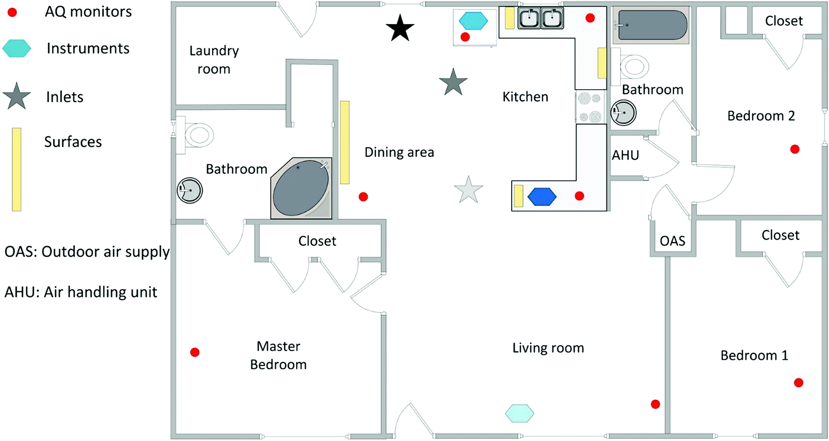 | ||
| Fig. 1 The UTest house floor plan includes a large open living room and kitchen space, including a sink and stove. The markers indicate instrument/inlet general locations. The bathroom doors were sealed with the master bathroom's exhaust fan left on; all other interior room doors were kept open. Three sets of large instruments were maintained inside the house (light blue hexagon in living room: HOx, HONO and spectral radiometer measurements; medium blue hexagon in kitchen: NH3 measurement; dark blue hexagon between kitchen and living room: aerosol and biological aerosol size distribution measurements). Low-cost air quality monitors were placed on top of the cupboards separating the kitchen from the living room area, and in the living room and bedrooms (red circles). Multiple vertical sampling surfaces were placed in the dining area and kitchen (yellow bars). Inlets for external sampling were located in the kitchen area (stars; black: SVTAG inlet; light grey: O3, NOx, SO2, CO2 and GC measurements of VOCs; medium grey: all other measurements). The locations of the outdoor air supply and air handling unit are indicated. The dishwasher is under the counter to the left of the sink, and the refrigerator between the sink and SVTAG inlet. | ||
2.1 House ventilation and household state monitoring
A dedicated outdoor air supply system was operated to keep the house positively pressurized relative to outdoors whenever the doors and windows were closed so as to minimize temporal variations in house ventilation rate driven by temperature differences and wind. This system delivered a constant outdoor air flow, which provided an average ± standard deviation air change rate (ACR) of 0.5 ± 0.1 h−1 when the doors and windows were closed. This outdoor air was supplied into the house near the return of the air handling unit of the HVAC system. Thus, incoming outdoor air was mixed with the room air at the air handling unit's return, and then conditioned by the HVAC system before being dispersed through the house.Apart from providing mechanical ventilation, major elements of the UTest House HVAC system are representative of a typical residential system, providing cooling, dehumidification and air circulation functions. For the HOMEChem campaign, the fan in the air handler of the HVAC system was set to operate continuously, regardless of heating or cooling demand, moving air through the HVAC system at a flow rate of 2000 m3 h−1 (equivalent to 8 house volumes per hour) so as to provide consistently rapid mixing throughout the house. A thermostat controlled the on/off cooling functions of the HVAC system as needed to maintain air temperature within the desired range. The filters in the outdoor air supply and air handling unit were removed to prevent measurements from being affected by filter type and filter conditions. As a consequence of the absence of an HVAC filter, indoor concentrations of particles and reactive trace gases during unperturbed, background periods may be somewhat higher than would have been the case in the presence of a filter. The exhaust hood above the stove was not operated during this study.
To facilitate internal air mixing, all interior doors were kept open throughout the HOMEChem study; the only exceptions were doors to both bathrooms and all closets, which were kept closed. Volunteers used only the master bathroom during experiments. The exhaust fan in this bathroom was kept on during the entire campaign to ensure that air entering the bathroom exited through the fan to the outside, thus minimizing emissions of stored cleaning products from entering the house air space. To enhance mixing in the living and kitchen area, a ceiling fan in the living room was on during the entire campaign. During experiments, all outside doors and windows were closed unless specified otherwise.
The test house was outfitted with 39 wireless sensors (see Table S3† for locations; SmartThings, Inc., Mountain View, CA, USA) to monitor motion, window/door open/closed status, and appliance usage. Data loggers recorded temperature in the kitchen and relative humidity (Veris HD2XVSX sensor, accuracy ±2% between 10 and 80% RH) in the living room. Additional sensors measured air temperature and CO2 levels in all rooms, and temperature and relative humidity at the inlet of the air handling unit, in the air supply duct after the air handling unit, and in the outdoor supply air. We also measured interior surface temperatures at 40 locations on the walls, floor and ceiling (Omega 44033 thermistor; accuracy of ±0.1 °C). Spectrally-resolved solar irradiance was measured with an Ocean Optics USB4000 (1 minute average, <15% error; fiber optic cable coupled with a cosine corrector), and alternated measurements between the living room and kitchen windows. Additional experiments investigated the spatial variability of light intensity and the contributions of diffuse and reflected light on total indoor spectral irradiance.
The air conditioning (AC) setpoint temperature was 25 °C for the kitchen and living area throughout the study period with the exception of a few specified periods with either no AC or a higher setpoint. Large occupancy and intensive cooking events, combined with heat gain from outdoors, sometimes exceeded the cooling capacity of the AC system and sporadically caused increases in indoor temperature above the setpoint. In addition to cooling, the air conditioning coils provided dehumidification through condensation when the thermostat called for cooling. An additional small-capacity dehumidifier positioned in series with the air handling unit provided continuous dehumidification, helping to prevent large variations in relative humidity. During experimental days, the kitchen and living area temperature was 25 ± 2 °C (average ± standard deviation) and the RH was 57 ± 6%. When windows and doors were opened and the air conditioner was turned off, the indoor temperature was 31 ± 3 °C. Throughout the entire HOMEChem study, indoor temperature ranged from 23 °C to 36 °C, while the relative humidity (RH) ranged from 43% to 82%. In contrast, outdoor temperature ranged from 20 °C to 38 °C (average ± standard deviation of 29 ± 4 °C) and RH ranged from 36% to 98% (71 ± 17%) during HOMEChem.
2.2. HOMEChem experimental design
HOMEChem experiments followed two approaches: sequential experiments and layered experiments. Sequential experiments repeated similar activities throughout the day, interspersed with periods of enhanced ventilation via window opening. Sequential experiments aimed to investigate emissions and short-term chemical processes following specific, isolated activities. Layered experiments included different cooking and cleaning activities performed throughout the day with no interspersed window opening. Layered experiments allowed emissions from multiple activities to interact in the house over longer periods of time. Layered experiments were designed around scripts to simulate real-life use of a home. The major event types investigated during HOMEChem were cooking, cleaning, and variable human occupancy (including the use of personal care products). Ventilation rates were also deliberately manipulated in some experiments through the opening and closing of doors and windows.We combined the experiment types into six day-long categories: (1) unoccupied background, (2) sequential experiments (cooking, cleaning, occupancy, ventilation), (3) layered experiments, (4) Thanksgiving, (5) maintenance, and (6) open house (one day) (Fig. 2). Unoccupied days involved no perturbation to the house, with no volunteers or researchers entering the house. Maintenance days typically included specific tests or additional experiments. Detailed schedules are provided in the ESI† (§S6).
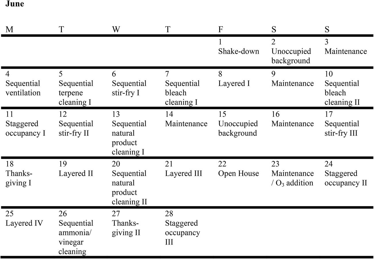 | ||
| Fig. 2 Experimental schedule for HOMEChem. | ||
The sequential ventilation experiments of 4 June entailed seven replicates of two steps: (i) opening doors and windows and operating several household box fans; (ii) after 30 minutes, closing windows and doors, turning off fans and leaving the house unoccupied for 90 minutes. For cooking and cleaning sequential days, in which each perturbation activity (e.g. mopping or stir-fry) typically lasted 10–40 minutes, we opened doors and windows two hours after the start of the activity, closed them after 30 minutes, and then waited another 30 minutes before repeating the activity.
For sequential cooking experiments, the experimental meal was a vegetable stir-fry. Volunteers cooked the stir-fry four times per day on three days, alternating between a propane stove and an electric hot plate as heat sources, and an aluminum wok and cast iron skillet as cooking surfaces. For sequential cleaning experiments, volunteers mopped the vinyl floors in the kitchen and living room with four cleaning products: (1) a commercial bleach solution, (2) a commercial product advertised as “all natural”, (3) a pine-scented commercial product, and (4) a vinegar solution. Volunteers preceded or followed the vinegar mopping with wiping windows, tables, and countertops using an ammonia solution. Different volunteers conducted replicated activities following detailed instructions regarding volume of vegetables, sauce and rice cooked; cooking temperature and time; and time spent mopping. Volunteers mixed the cleaning solvents according to manufacturer's instructions, and weighed mopping solutions before and after mopping.
The three staggered occupancy days followed a different schedule from other sequential experiments. Up to 12 occupants entered the house in groups of 2–3 at 15 minute intervals. After 75 minutes, the volunteers left in the same order they entered, creating a stepwise increase and decrease in total occupancy (Fig. 3). After a two-hour break with windows and doors open to ventilate the house, volunteers repeated the experiment. On the first occupancy day, volunteers wore minimal personal care products, opting for products advertised as ‘all natural’ or ‘organic’. On the second occupancy day, volunteers wore their ‘usual’ quantities and types of products. On the third day, volunteers wore generous (but not unrealistic) amounts and types of personal care products.
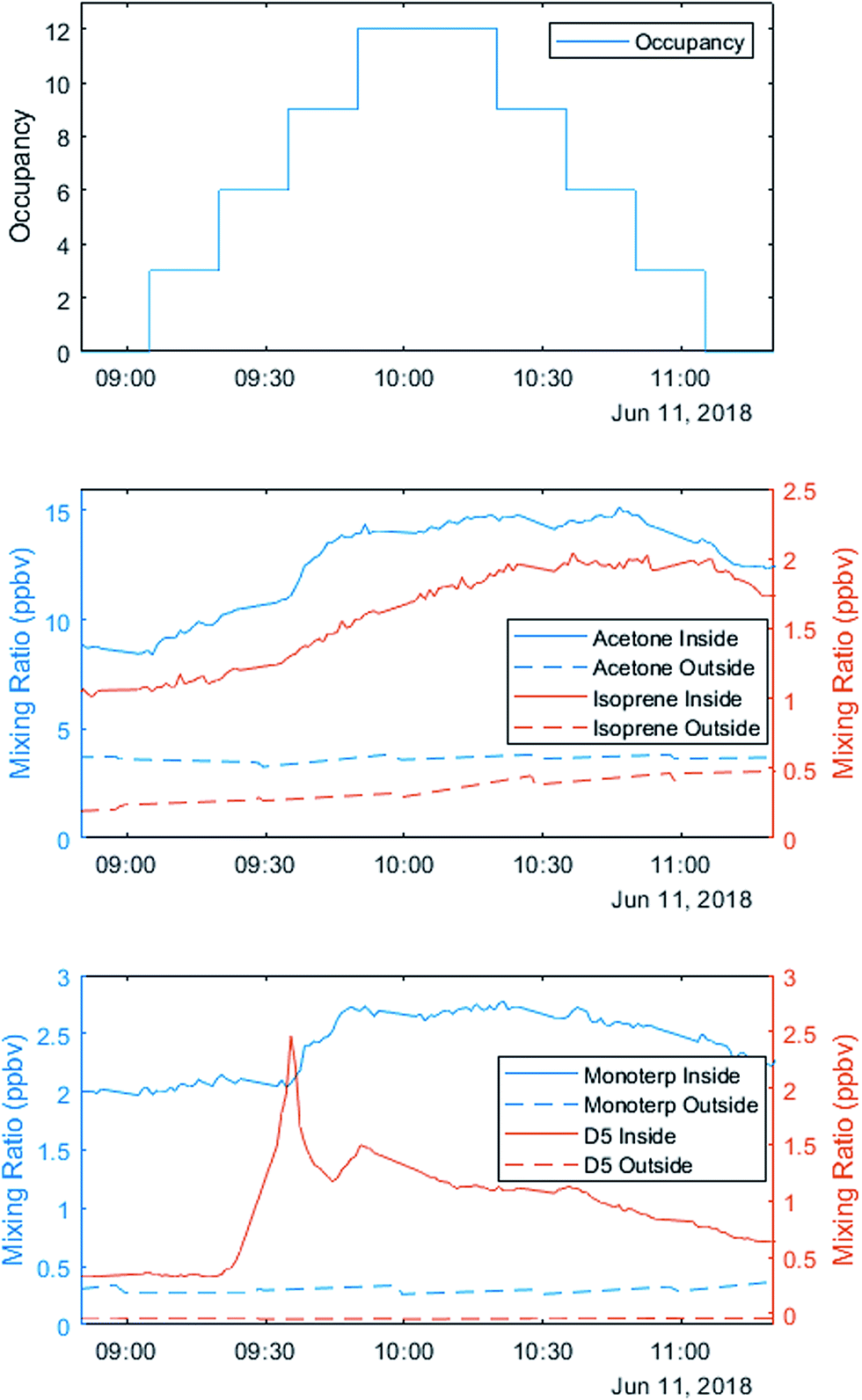 | ||
| Fig. 3 Occupancy was staggered on the three sequential occupation experiments. The first occupancy period on 11 June (minimal personal care product day) exemplifies the enhancement of acetone, isoprene, monoterpenes and the D5-siloxane from human emissions. | ||
Layered experiments involved three volunteers cooking, cleaning and occupying the house for 9.5 hours without opening the doors or windows. The layered day followed a prescribed schedule of cooking breakfast, mopping the floors with a terpene cleaner, cooking lunch, wiping the kitchen counter surfaces with commercial ‘bleach free’ wipes, making coffee and toast, cooking dinner, operating the dishwasher, mopping with a bleach solution, and exiting the house. Similar to the primary layered experiments, Thanksgiving days simulated the traditional American holiday activity with four volunteers cooking a turkey dinner with trimmings for 10+ additional volunteers, who arrived, ate and cleaned up. On maintenance days, researchers calibrated instruments and ran additional experiments (e.g. instrument intercomparisons). During the Open House, 40+ individuals visited the HOMEChem site and entered the test house, with no specific experiments performed on that day. Exact numbers of attendees and the times of their presence indoors were not recorded during the open house event.
Volunteers conducted supplemental experiments during evenings and on maintenance days. These included particle-generation events (e.g. cooking toast on the evening of 26 June; releasing Arizona test dust on the evenings of 22 and 28 June), ozone addition experiments (three experiments on the night of June 23 and three experiments on the night of June 24), and a temperature ramp (house temperature setpoint ramped from 24.4 °C down to 17.8 °C and back to 24.4 °C over the course of nine hours on June 28–29).
All major appliances were installed in the UTest house more than a year prior to HOMEChem. The oven had been unused until May 2018.
2.3 Volunteer information
Researchers from the HOMEChem science team performed all activities. An experimental log retains time-dependent numbers of occupants, but identities and any potentially identifying information (e.g. age, gender) of volunteers are not available. Volunteers recorded personal care products used only during sequential occupancy experiments. The Institutional Review Board's (IRB) human research review was waived for the HOMEChem study because the only data recorded was the number of occupants in the house and the types of personal care products used in sequential occupancy experiments, with no ties to personal identifying information.2.4 Chemical measurements
The HOMEChem study included an array of real-time instruments with inlets measuring both indoor and outdoor air (Tables 1–4). Table 5 summarizes off-line sample collection for surface composition, passive sampling and aerosol chemistry. The study also included seven different low-cost air quality monitors (five commercially available and two research prototype units), with replicated monitors deployed in different locations throughout the house (ESI Table S2†).| Measured species | Sampling location | Instrument | Time resolution | Uncertainty | Notes |
|---|---|---|---|---|---|
a All gas phase inlets were made of 0.635 cm (1/4′′) o.d. PFA tubing unless stated otherwise. Alternating sampling locations were controlled by integrated valve switching, typically 25 minutes indoors followed by 5 minutes outdoors.
b
 refers to the sum of HO2 radicals plus a fraction of certain RO2 radicals.27 refers to the sum of HO2 radicals plus a fraction of certain RO2 radicals.27
|
|||||
| O3 | Alternating living room & outdoors | 2B Technologies model 202 | 10 s | LOD: 1.2 ppb | Two 6-point calibrations during HOMEChem with 2B Technologies model 306 O3 generator |
| Error: 5% | Inlet lengths: 17.3 m indoor, 8.6 m outdoor | ||||
| O3 | (i) House air return | 2× Horiba APOA 370 ambient ozone monitor | 10 s | LOD: 0.5 ppb | Cross flow modulation type, non-dispersive ultraviolet absorption method |
| (ii) House air supply | |||||
| NO, NO2 | Alternating living room & outdoors | Thermo Fisher model 42i TL with home-built blue light converter for NO2 detection | 2 min | LOD: 2.3 ppb | Calibrated using external 11-point calibration for 0–600 ppb range |
| Error: 5% | Inlet lengths: 17.3 m indoor, 8.6 m outdoor | ||||
| NO2 | Living room | Environnement, S.A. Cavity attenuated phase shift spectroscopy (CAPS) NO2 monitor24 | 1 min | LOD: 0.1 ppb | Linearity checks before and after campaign, calibration after campaign. Details in ESI Section 7 |
| NH3 | Kitchen | Picarro G2103 | 1 min | LOD: 0.5 ppb | Instrument calibrated by Picarro immediately prior to deployment |
| Error: 5% | |||||
| SO2 | Alternating living room & outdoors | Teledyne LIP | 1 min | LOD: 0.05 ppb | Internal low and high span calibrations with SO2 cylinder; see ESI Section 5 for additional details |
| Error: 5% | Inlet lengths: 18.4 m indoor, 7.9 m outdoor | ||||
| CO2 | Alternating living room & outdoors | LICOR model LI- 840A | 1 s | LOD: 10.2 ppm | Internal low and high span calibrations for 0–6500 ppm during HOMEChem. External post-campaign 9-point calibration |
| Error: 4% | Inlet lengths: 18.4 m indoor, 7.9 m outdoor | ||||
| CO, CO2, CH4 | Alternating kitchen & outdoors | Picarro G2401 | 1 min | Uncertainty | Instrument calibrated prior to deployment and upon return |
| *Inlet shared with HR-AMS | CO2 < 50 ppb | Inlets: 9.5 mm (3/8′′) o.d. stainless steel tubing | |||
| CO < 2 ppb | |||||
| CH4 < 1 ppb | |||||
| CO2, H2O | Alternating kitchen & outdoors | LICOR model LI-840A | 1 s | LOD | Inlet lengths: <0.5 m of PFA Teflon tubing in addition to inlet tubing described in the EESI-ToF-MS description (Table 3) |
| CO2: <1 ppm | |||||
| H2O: <10 ppm | |||||
HO2,  b b |
Living room window | LIF FAGE25,26 | 1 min | LOD: 1 × 10⁷ molec per cm3 | Calibrated using water vapor photolysis method before, during, and after campaign |
| OH, HONO | Living room window | LP/LIF-FAGE25 | 15 min | LODs | OH calibrated using water vapor photolysis method before, during, and after campaign. HONO calibrated before and after campaign |
| OH: 1 × 10⁶ molec per cm3 | |||||
| HONO: 50 ppt | |||||
| Measured quantity | Sampling location | Instrument | Time resolution | Notes |
|---|---|---|---|---|
| a All gas phase inlets were made of 0.635 cm (1/4′′) o.d. PFA tubing unless stated otherwise. Alternating sampling locations were controlled by integrated valve switching, typically 25 minutes indoors followed by 5 minutes outdoors. | ||||
| VOCs | Living room | VOC 4-channel GC28 | 50 min | C2–C8 hydrocarbons; BTEX; speciated monoterpenes (limonene, α-pinene, β-pinene); CFCs; C1–C5 alkyl nitrates |
| Daily two-point calibrations with multi-component whole air standards. | ||||
| Inlet lengths: 13.2 m | ||||
| VOCs | Alternating kitchen & outdoors | PTR-TOF-MS4,29 | 1 min | Target species directly calibrated; all other species concentrations calculated based on theoretical transmission |
| Inlet lengths: 8.4 m | ||||
| Oxidized VOCs, halogenated species, N2O5 | Alternating kitchen & outdoors | Iodide CIMS30 | 1 s | On-line calibration of formic, acetic, propionic, butyric, and pentanoic acid using permeation tubes |
| Off-line calibrations include Cl2, ClNO2, HOCl, N2O5, multiple organic acids | ||||
| Inlet lengths: 7 m indoor, 5 m outdoor | ||||
| Organic acids, HONO | Alternating kitchen & outdoors | Acetate CIMS20 | 1 s | Calibrated species: HONO;31 HNCO;32 formic, propionic, butyric, and pentanoic acid (via permeation tubes) |
| Inlet lengths: 10 m indoor, 8 m outdoor, shared inlet with iodide CIMS | ||||
| Gas and particle composition and partitioning | Kitchen (switched to outdoors on a few nights) | FIGAERO-CIMS33 with iodide ionization | 1 s gas phase; | Inlet lengths: 2.1 m outdoor, 8.4 m indoor (PFA for gases, 9.5 mm o.d. stainless steel tubing for particles) |
| 1 h for particle phase | Calibrated by aerosol spray for levoglucosan, malonic acid and by drops onto FIGAERO filter for multiple organic acids | |||
| Gas and particle phase semi-volatile organic compounds | Alternating kitchen & outdoors | SV-TAG: thermal desorption aerosol gas chromatography with online derivatization11,34 | 1 h | Calibration via internal standards and >100 authentic external standards |
| 20 minute sampling window through stainless steel tubing (16 mm (5/8′′) o.d.; inlet lengths 2 m indoor, 3.7 m outdoor) | ||||
| Measurement | Instrument | Inlet | Notes |
|---|---|---|---|
| a Alternating sampling locations were controlled by integrated valve switching, typically 25 minutes indoors followed by 5 minutes outdoors. Time resolution represents final data product. | |||
| Submicron non-refractory particle composition | HR-AMS35 | Alternating kitchen & outdoors (9.5 mm (3/8′′) o.d. stainless steel tubing), sample air dried with MD700 Nafion dryer | 1 min time resolution |
| LOD: 0.312 μg m−3, 0.024 μg m−3 (chloride), 0.040 μg m−3 (sulfate), 0.024 μg m−3 (nitrate), 0.394 μg m−3 (ammonium) | |||
| Submicron non-refractory particle composition with thermal denuder | TD-TOF-ACSM36 | Alternating kitchen & outdoors (9.5 mm (3/8′′) o.d. copper tubing) | 40 s time resolution |
| LOD: <0.2 μg m−3 for particle species | |||
| Submicron non-refractory particle composition | ACSM37 | Outdoor inlet | 30 min time resolution |
| (3 m length × 6.3 mm (1/4′′) o.d. copper with PM2.5 cyclone and diffusion dryer) | Sampled indoors from 17–20 Jun and on 26 Jun (8 m of 6.3 mm (1/4′′) o.d. copper) | ||
| Speciated organic aerosol composition | EESI-ToF-MS | Alternating kitchen and outdoors | 5 s time resolution |
| LODs: 350 ng m−3 for levoglucosan and 1.20 μg m−3 for oleic acid | |||
| Particle absorption in UV-IR | 2× microAeth MA200![[thin space (1/6-em)]](https://www.rsc.org/images/entities/char_2009.gif) 38 38 |
(i) Kitchen | 1 min time resolution |
| (ii) Outdoors | 5 wavelength UV-IR absorption | ||
| 1.5 m inlet with diffusion dryer | |||
| Black and brown carbon | AE-33 Aethalometer39 | Alternating kitchen and outdoor (inlet shared with HR-AMS, dried with MD700 Nafion drier) | 1 min time resolution |
| 7 wavelength UV-IR absorption | |||
| Metal content of PM2.5 | Aerosol spark emission spectrometer40 | Kitchen | 2 min to 4 h time resolution |
| Size range | Instrument | Inlet location | Notes |
|---|---|---|---|
| a Acronyms: SMPS = scanning mobility particle sizer, EC = electrostatic classifier, DMA = differential mobility analyzer, CPC = condensation particle counter; UHSAS = ultra high sensitivity aerosol spectrometer; SEMS = scanning electrical mobility system; APS = aerodynamic particle sizer. | |||
| 1–4 nm | Airmodus A11-nCNC system41 | Kitchen | 5 min per scan |
| 4–105 nm | SMPS (TSI 3080 EC + 3085 nano-DMA + 3788 water CPC) | Kitchen | 5 min per scan |
| 11–533 nm | SMPS (TSI 3080 EC + 3081 long-DMA + 3787 water CPC) | Kitchen | 5 min per scan |
| 17 nm–580 nm | SMPS (TSI 3080 EC + 3081 DMA + 3075 CPC) | Alternating kitchen and outdoor | 2.5 min |
| Inlet shared with EESI-TOF-MS | |||
| 130 nm–3 μm | 4 × POPS (portable optical particle sensors, Handix Scientific)42 | (i) Kitchen | 1 s |
| (ii) Living room | |||
| (iii) Bedroom 1 | |||
| (iv) Outside (1–23 June) and kitchen counter (24–28 June) | |||
| 60–1000 nm | UHSAS (Droplet Measurement Technologies)43 | Alternating kitchen & outdoor inlet | 1 s |
| Inlet shared with HR-AMS | Likely saturated at concentration > 3000 particles cm−3 | ||
| 10–946 nm | SEMS (Brechtel Manufacturing incorporated model 2002) | Outdoor | 30 min |
| Inlet shared with ACSM | |||
| 500 nm–20 μm | 2× APS (TSI 3321)44 | (i) Kitchen | 1 min per scan |
| (ii) Outdoor | Minimum particle count: 0.001 particles cm−3 | ||
| 500 nm–15 μm (fluorescent particles) | UV-APS (Ultraviolet APS, TSI 3314)45 | Kitchen | 1 min |
| PM2.5 | DustTrak (TSI 8520) | Kitchen (above kitchen cabinets) | 1 min. Data collection June 23–29 |
| Measurement | Surface material/location | Measurement | Notes |
|---|---|---|---|
| Spatially-resolved metabolites and microbial communities46 | Multiple surfaces throughout the kitchen living room and bathroom | HPLC MS/MS | Samples collected on 31 May and 29 June |
| 16S sequencing | |||
| Passive VOC samplers46 | Multiple surfaces throughout the kitchen living room and bathroom | GC/MS | Samples collected on 1 and 29 June |
| Surface nitrite20 | Glass/dining room | Surface wipes with nylon filter followed by Griess test using UV-vis |
Samples collected and analyzed daily |
| Surface depositions | Glass/dining room | AFM/AFM-IR, Orbitrap MS, ICP-MS | Samples collected after exposure durations of 3 h, 24 h and multiple days |
| Surface depositions47 | Glass & painted drywall substrates in dining area | Functional groups | 12 × 24 h samples |
| Metal content of PM2.548,49 | Sample collected on 37 mm Teflon filters from inlets installed indoors (kitchen) and outdoors. (Sample train included 2.5 μm impactor) | Inductively coupled plasma mass spectrometry (ICP-MS) | Indoor samples collected twice daily from 7–28 June; outdoor samples collected from 17–28 June |
| Surface depositions50 | Glass/dining room on the wall and above stove | Offline HR-ToF-AMS and ESI FT-ICR | Samples extracted with acetonitrile |
| Particle samples | Filter collection | SEM | |
| Passive SVOC samplers | Sorbent material (PDMS) | GC-MS | Daily sample collection on 18 days |
3. Case studies
The HOMEChem dataset provides a wealth of information on not only trace gas and particle concentrations inside and outside the test house, but also surface composition and the role of typical activities in altering this chemistry. A complete synthesis of HOMEChem data is beyond the scope of this initial overview. Instead, we describe several case studies that demonstrate the utility of this dataset for investigating indoor chemistry in a residential environment. The first case study contrasts indoor and outdoor concentrations of trace gases, particles and photolysis rates, providing chemical context for the HOMEChem study. The second case study demonstrates cooking as a substantial, yet chemically diverse, source of indoor particles. The third case study highlights the complexity of multiple sources in contributing to VOCs in general, and organic acids in particular. The fourth case study highlights new opportunities in indoor chemistry measurements by comparing multiple methods for characterizing films deposited on indoor surfaces. The fifth case study demonstrates the challenges of measuring even relatively abundant trace gases, specifically NO2, in chemically complex indoor air.3.1 Case study 1: contrasting indoor vs. outdoor air
Differences observed between indoor and outdoor air composition were generally consistent with findings in previous studies. For example, with the exception of periods impacted by cooking events, accumulation mode particle concentrations were lower indoors than outdoors during HOMEChem (Fig. S6 and S10†). However, indoor particle concentrations were markedly elevated during cooking events, for example reaching hundreds of μg m−3 during stir-fry events. Whereas accumulation mode particles commonly dominate the PM2.5 aerosol mass concentration (i.e. mass of particles with diameter <2.5 μm) in the outdoor environment, ultrafine (i.e. <100 nm; PM0.1) particles can be so numerous indoors during cooking events that they influence PM2.5.In the absence of ozone generating devices, O3 has long been known to be lower indoors than outdoors – and HOMEChem data are no exception.51,52Fig. 4 compares indoor and outdoor distributions of O3 and other inorganic trace gases. As most of the data points were collected during unoccupied, unperturbed conditions, peaks in the histogram for indoor data represent baseline conditions. Outdoor O3 levels varied through the diel cycle, peaking in the mid-afternoon, consistent with photochemical generation typically encountered in urban environments. Ozone was consistently lower indoors than outdoors (Table 6). Under closed-house conditions, O3 exhibited a relatively steady mixing ratio of 5 ± 3 ppb independent of time of day, increasing only when the house was opened or when O3 was deliberately injected. At night, outdoor O3 reached minima of 10–15 ppb, two to three times larger than the concurrent indoor mixing ratio.
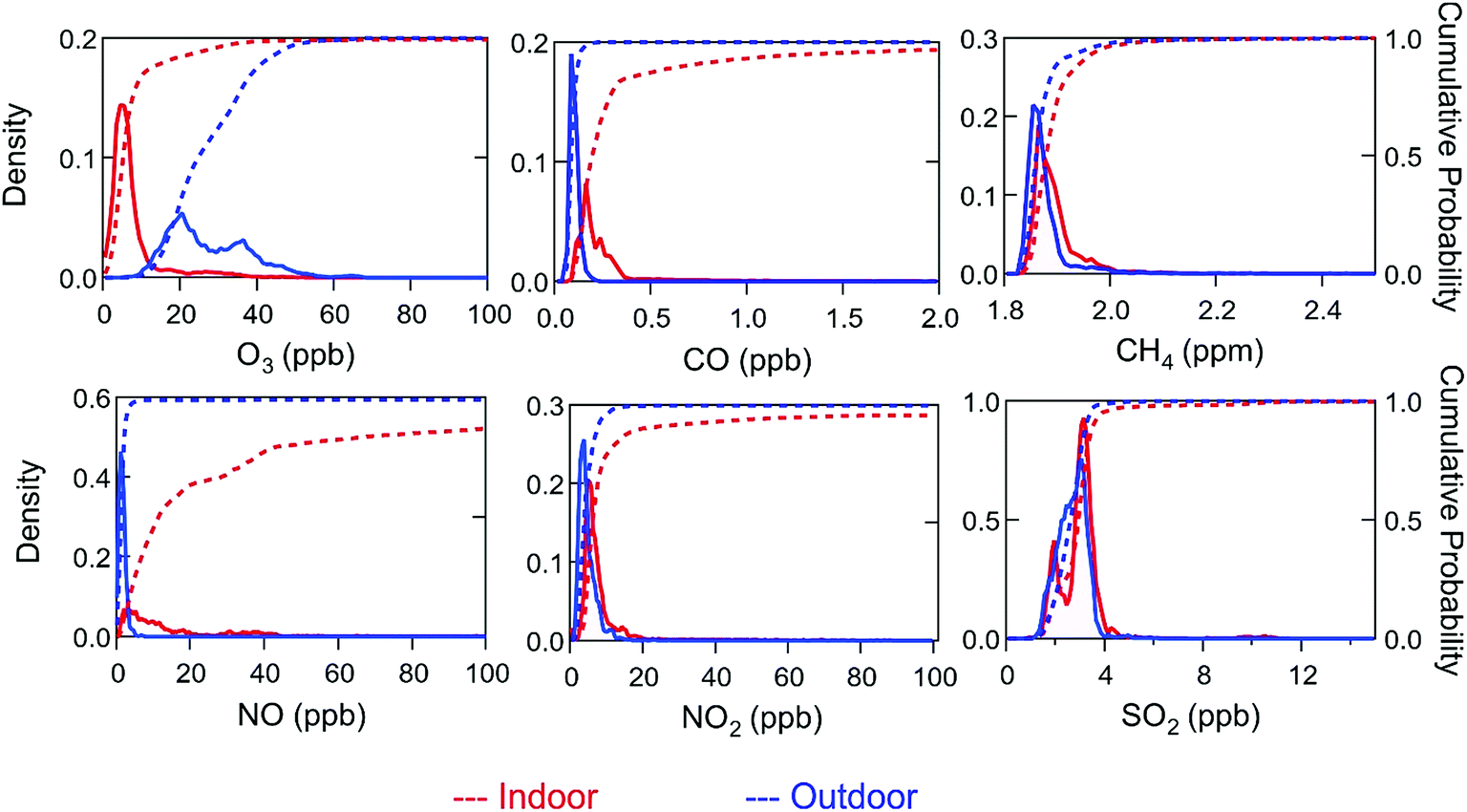 | ||
| Fig. 4 Normalized probability (solid line; left axis) and cumulative probability (dashed line; right axis) distributions of trace gas data for the entire HOMEChem experiment for indoor (red) and outdoor (blue) measurements. Mixing ratios of O3 (2B Technologies UV absorption measurement; 10 s averages), CO (Picarro 2401, 1 min average), CH4 (Picarro 2401, 1 min average), NO (chemiluminescence measurement, 2 min average), NO2 (blue light converter + chemiluminescence, 2 min average), and SO2 (pulsed fluorescence measurement, 1 min average). | ||
| Indoor mean ± standard deviation | Outdoor mean ± standard deviation | |
|---|---|---|
| O3 (ppb) | 8 ± 18 | 28 ± 11 |
| NO (ppb) | 50 ± 130 | 1.7 ± 1.4 |
| NO2 (ppb) | 7 ± 27 | 5 ± 3 |
| CO (ppb) | 0.4 ± 0.8 | 0.1 ± 0.04 |
| SO2 (ppb) | 3 ± 1 | 2.7 ± 0.6 |
| CO2 (ppm) | 670 ± 530 | 413 ± 8 |
| CH4 (ppm) | 1.90 ± 0.05 | 1.88 ± 0.05 |
In contrast to O3, several other trace gases (i.e. NOx, CO, CO2) were typically higher indoors than outdoors (Table 6). These compounds were clearly influenced by indoor activities, increasing when the gas stove or oven was in use, and, in the case of CO2, from metabolic emissions when humans occupied the house. During the Thanksgiving experiments, NO reached a maximum of 1085 ppb, NO2 rose to 105 ppb and CO2 peaked at slightly above 4000 ppm. The elevated NO2 levels are comparable to the 1 hour 100 ppb outdoor air quality standard set by the US EPA, although we note that these concentrations only persisted for short periods (minutes to hours) during HOMEChem. Indoor CO (range of 0.1 to 10.2 ppb) was higher than outdoor (range of 0.1 to 2.4 ppb). Indoor enhancements in CO and NOx were likely due primarily to stove/oven use and the associated gas pilot lights. Indoor CO never exceeded the NAAQS 1 hour average limit of 35 ppm or 8 hour average limit of 9 ppm.
Background (unoccupied, unperturbed) indoor NO and NO2 mixing ratios were similar (5.2 ± 6.4 ppb NO and 5.5 ± 2.1 ppb NO2). The much higher NO:NO2 ratio indoors than outdoors is consistent with most of the indoor NOx originating as NO emitted from the gas stove and oven pilot lights. Outdoors, NO would rapidly reach a steady-state with NOx dominated by NO2, but the low indoor O3 concentrations enable the relatively high indoor NO:NO2 ratio to persist. The high indoor NO:NO2 ratios during cooking events contrast to older reports of relatively high emissions of NO2 from gas stoves, but we note that reported emission ratios of NO:NO2 from indoor combustion sources span a large range.53–55 Higher NO:NO2 ratios have been observed from gas-powered appliances in more recent studies.56,57 Appliance design may have changed resulting in higher NO:NO2 emissions, or differences may be driven by measurement technology: older measurements often utilized catalytic NO2 converters that are subject to interferences from HONO, PAN, HNO3 and other oxidized nitrogen compounds.58 High indoor NOx and CO2 and low O3 (relative to outdoor concentrations) are consistent with previous residential studies in the US.59–62
Indoor and outdoor concentrations of CH4 were similar (ranges 1.8–2.4 ppm indoors and 1.8–2.7 ppm outdoors) with no clear diel cycle. Similarly, sulfur dioxide (SO2) showed no diel cycle or differences in indoor and outdoor concentrations. Indoor SO2 peaked at 11.5 ppb on 27 June during the Thanksgiving experiment. Gas stoves and matches are known sources of particulate sulfate, and are likely indoor SO2 sources during HOMEChem.63
Spectral irradiance, and thus photolysis rate constants, are substantially lower indoors than outdoors. For example, HONO photolysis rate constants (JHONO) are typically 1–2 orders of magnitude lower indoors than outdoors at any given time. Indoor temporal trends in photon fluxes and photolysis rates depend on solar zenith angle, presence of clouds, and placement of windows, causing strong spatial heterogeneity and differences in diel patterns not only between indoor and outdoor environments, but also among different locations indoors (Fig. 5). These spatial gradients may influence photolysis rates for photolabile molecules such as NO2. The resulting photochemical production of O3 is likely less than the physical supply by transport of outdoor air under most conditions, but the irradiance and NO2 measurements suggest both spatial and temporal variability in O3 production rates in the indoor environment.
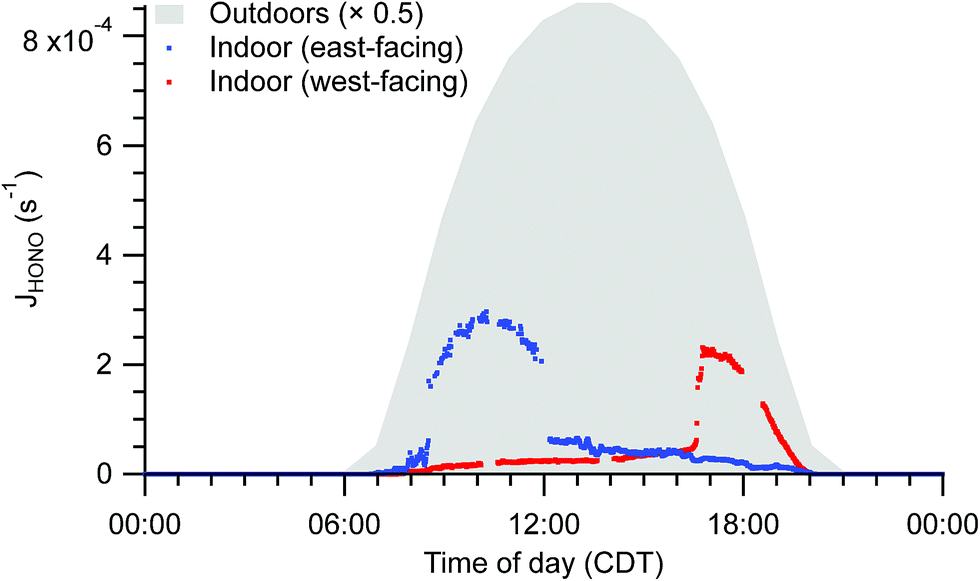 | ||
| Fig. 5 Indoor photolysis rate constants of HONO calculated from solar spectral photon fluxes measured near to the east-facing and west-facing windows under clear sky conditions. Photon fluxes were determined from measured spectral irradiance. Outdoor HONO photolysis rate constants based on tropospheric ultraviolet and visible (TUV) radiation model results are shaded in grey for comparison.64 | ||
3.2 Case study 2: indoor PM2.5 and cooking
Cooking activities were the primary source of indoor submicron particles during HOMEChem. While particle emissions from cooking have been studied extensively, a major focus has been on particles from solid fuel combustion (e.g. biomass and coal), which are still used by more than a third of the world's population.65,66 In developed countries, cleaner cooking fuels, such as natural gas, propane, and electricity, emit less particle mass compared to solid fuels. Nevertheless, cooking is a well-known indoor particle source.67,68 High particle mass concentrations were observed during HOMEChem cooking activities, relative to outdoor levels. The maximum size-segregated particle mass concentrations (i.e. PM0.1, PM0.5, PM1, PM2.5, PM10, and PM20) observed during each meal highlight the variation with cooking type (Fig. 6a). The highest particle mass concentrations on layered days occurred during breakfast. The PM2.5 level exceeded 200 μg m−3, with fine particles accounting for >70% of the total observed particle mass. The smaller size modes, PM0.1 and PM0.5, were also substantially elevated, exceeding 30 μg m−3 and 170 μg m−3, respectively, during breakfast preparation. (These mass concentrations are derived from number-based measurements using the SMPS and APS.) Fig. 6a assumes a single particle density of 1 g cm−3, consistent with hydrocarbon-like organic aerosol, although atmospheric aerosol density varies from 0.9–1.8 g cm−3 depending on composition. Of course, these reported values represent only one house with a particular pattern of cooking under a single set of ventilation conditions.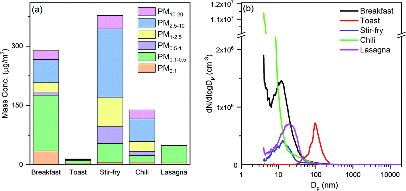 | ||
| Fig. 6 (a) The highest mass concentrations by size (PM0.1, PM0.5, PM1, PM2.5, PM10, and PM20) during the preparation of each meal. (b) Particle number size distributions (electrical mobility size: 4 nm–532 nm; aerodynamic size: 542 nm–19.8 μm) corresponding to the highest PM mass concentrations recorded during different types of meals cooked. Mass calculations from size distribution measurements assume a constant aerosol density of 1 g cm−3. | ||
Different cooking activities resulted in different particle size distributions (Fig. 6b). Particles less than 20 nm in diameter dominated the number size distributions during cooking with the stove, oven, or hot plate, consistent with previous measurements.69 Toasting bread in an electric toaster was the only cooking activity in which particle number concentrations were not dominated by particles smaller than 20 nm.
During cooking events, the HR-AMS detected substantial amounts of organic aerosol (often >100 μg m−3). Outdoors, cooking-associated organic aerosol (COA) can be identified in aerosol mass spectra through ratios of tracer ions and component factor analysis; COA has also been observed to be transported into the indoor environment from outdoors.22,70–72 During HOMEChem, COA size distributions, concentrations, and bulk mass spectral profiles varied considerably with meal type and preparation method (e.g. gas stove vs. hot plate vs. toasting vs. oven). The high time resolution of the HR-AMS enables differentiation of submicron aerosol composition throughout the cooking process. Many HOMEChem meals involved placing food into hot oil, and one involved splashing water into hot oil to aerosolize oil (“oil splash”). We contrast composition and mass spectra between aerosolized oil (Fig. 7a) and stir-fry COA produced when vegetables are added to the oil (Fig. 7b).
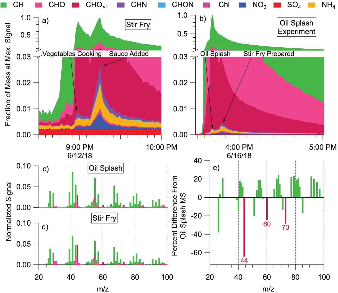 | ||
| Fig. 7 Time series of non-refractory submicron aerosol composition from (a) cooking stir-fry and (b) aerosolized oil during an oil splash. Stacked times series of species detected by the HR-AMS are scaled to the maximum concentration of each event for comparison, with key activities labeled. Normalized organic mass spectra for (c) oil splash and (d) stir-fry experiments show the CxHy+ ions in green and CxHyOz+ ions in magenta. The normalized signal represents each ion family's fractional contribution to total aerosol mass scaled to the maximum concentration observed during the given experiment. The stir fry aerosol mass spectrum (d) is an average of normalized mass spectra calculated over the duration of each stir fry cooking event (n = 12), while the oil splash mass spectrum (c) is a 15 minute average taken after pure oil was heated and aerosolized by droplets of water added to the pan (n = 1). Frame (e) shows the percent difference oil splash versus stir-fry mass spectra [(oil MS − stir fry MS)/oil MS × 100%]. Aerosol mass is calculated as a normalized nitrate equivalent mass (i.e. assuming all masses have ionization efficiencies equal to nitrate in the HR-AMS; RIE = 1.0). | ||
The particles emitted during the oil splash and stir-fry experiments were dominated by organic molecules. Inorganic components (non-refractory nitrate NO3, sulfate SO4, chloride Chl, and ammonium NH4) comprised <3% of the average total aerosol signal. Sulfate concentration remained at background levels throughout cooking experiments, trending with outdoor concentrations, while aerosol mass of other inorganic components (NO3, Chl, NH4) increased. The CxHy+ family of organic ions comprised most of the aerosol mass for both the aerosolized oil and the food in stir-fry experiments, followed by CxHyOz+ ions, consistent with the fatty acid composition of cooking oils. Slight enhancements in CxHyN+ and CxHyON+ were observed in both experiments but contributed little to total particle mass (<1% of the total).
The mass spectra of stir-fry organic aerosol (Fig. 7d) shows a greater contribution of CxHyOz+ ions than the oil splash (Fig. 7c), likely due to the complex sugars and proteins originating from the vegetables being cooked and the added stir-fry sauce. The oil splash mass spectrum is dominated by CxHy+ ions, consistent with a primary source of long-chain hydrocarbons (e.g. m/z 41, 55, 69). However, the total organic aerosol mass spectra from oil versus food in oil are similar (Pearson's correlation coefficient, r = 0.97). Furthermore, separating the mass spectrum into the CxHy+ and CxHyOz+ ion families results in correlation coefficients of 0.99 and 0.94, respectively. The high correlation indicates that the mass spectral signature of the stir fry cooking aerosol is dominated by the contribution of cooking oil to the aerosol.
Tracer ion ratios provide additional insight into the COA chemistry. The abundance of COA is often indicated by a ratio of the signals at m/z 55:57 > 1, but other ion ratios such as m/z 41:43 may also differentiate COA by cooking method or meal.70,73 We found the 55:57 ratio to be 2.26 for the oil splash and 1.80 for the stir fry. These ratios are consistent with the 1.5–4 range observed during outdoor ambient and primary source studies.70,72,74,75 The relative difference between the oil splash and stir-fry mass spectra (Fig. 7e) contains strong negative CxHyO>1+ peaks at m/z 44, 60, and 73, indicating that these oxidized ions are emitted from the food ingredients, i.e. the vegetables and/or sauce.
Cooking is clearly an important aerosol source indoors, and has also been observed to be an important aerosol component outdoors in urban environments.72,76 These initial mass spectral comparisons from HOMEChem reinforce previous source studies70 and highlight the challenge in defining COA with one mass spectral ratio or factor. Outdoor COA is difficult to separate from hydrocarbon organic aerosol (HOA) due to the predominance of CxHy+ ions and spectral similarity between the two components.72 Preliminary analysis of the HOMEChem data suggests that specific ratios within the CxHy+ and CxHyOz+ families may help differentiate these otherwise similar spectra in future studies.
3.3 Case study 3: VOC sources
The comprehensive suite of instruments enables a detailed characterization of indoor VOCs at HOMEChem. It is clear from preliminary analyses that the sources and behavior of some VOCs, including the oxidized organic acids, are complex. Certain emission sources, such as cleaning product use and human metabolism, have expected effects on indoor VOCs. These features are well illustrated during the layered experiment days (Fig. 8). The gas stove was used three times throughout the day (breakfast, lunch, dinner), resulting in increases in NO, NO2, CO2, and ethyne (acetylene). (The gas stove used propane, and concentrations of this species varied substantially across layered days, suggesting a small fuel leak, possibly from the pilot light.) Ozone is consistently low (∼5 ppb), but the measurement signal rises slightly during bleach mopping events, possibly due to an interference. Mopping with pine-scented cleaner raised limonene levels, while mopping with bleach solution raised chloroform levels. Both isoprene and acetone are known human metabolic emissions, and concentrations of both species were elevated throughout each layered day. Isoprene shows a rapid drop after each bleach mopping event, consistent with consumption by chemical reactions. We note that the chemical signatures are consistent across the layered days despite the variability of outdoor conditions and expected internal variability in volunteer behavior, demonstrating the replicability of the HOMEChem experimental data (Fig. S7†). Concentrations of most VOCs and trace gases are similar during the same events on different days. For example, CHCl3 reaches a concentration maximum at the same time during bleach cleaning and at similar levels (1.23, 1.37 and 1.33 ppb). In contrast, while isoprene reaches similar maxima on the three days, the maximum concentration on the first layered day occurs during lunch cooking, while the maximum on the third layered day occurs during dinner.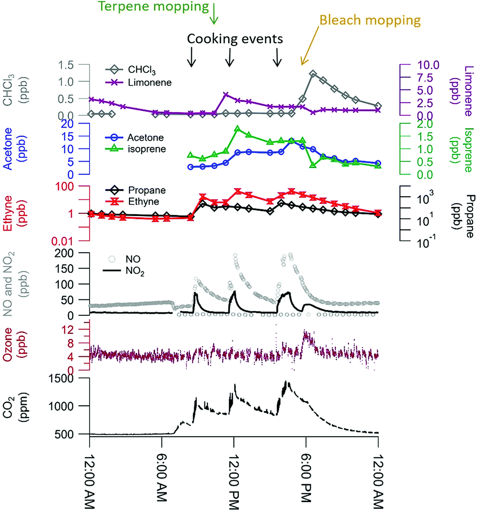 | ||
| Fig. 8 Trace gas data during a layered experiment day highlights influences of human occupancy, cooking, and cleaning perturbations. Researchers entered the house 7–7:30 am for instrument maintenance and preparation, accounting for the initial rise in CO2 (exhaled human breath) and drop in NOx (door opening brings in outdoor air). Three occupants remained in the house from 8:25 am through 5:45 pm (detailed schedule in ESI Section 6).† | ||
VOC observations on the variable occupancy days highlight the role of human sources. Metabolic sources of acetone correlate with the number of occupants, while monoterpenes and D5-siloxanes are likely emissions from personal care products (Fig. 3).
While hydrocarbons like limonene, propane, and isoprene varied following their expected cooking, cleaning and human emissions, the time series of organic acids displayed evidence of more complex sources and sinks. Organic acids are prominent in the outdoor atmosphere,30,77,78 but also have indoor sources, including human metabolism, building materials, and oxidation chemistry.79–81 Exchange of indoor and outdoor air means that outdoor sources may contribute to indoor air organic acid concentrations. Fig. 9 shows indoor and outdoor measurements of various gas phase organic acids during a lengthy background period from HOMEChem using iodide CIMS. No in-house experiments were performed during this period and occupancy was minimal, allowing us to explore indoor sources of these compounds from the building and its static contents. Indoor formic and acetic acid mixing ratios remain relatively stable throughout the background period, with an average indoor mixing ratio for formic acid of 30 ppb and acetic acid of 22 ppb. Both organic acids rapidly fluctuate ±10% around their mean mixing ratios in relation to HVAC cycling. These mixing ratios are comparable to levels previously reported in homes during summer. For example, Reiss et al.79 observed 8–33 ppb of formic and 9–88 ppb of acetic acid; Duncan et al.81 observed 10–30 ppb of formic and 10–40 ppb of acetic acid.
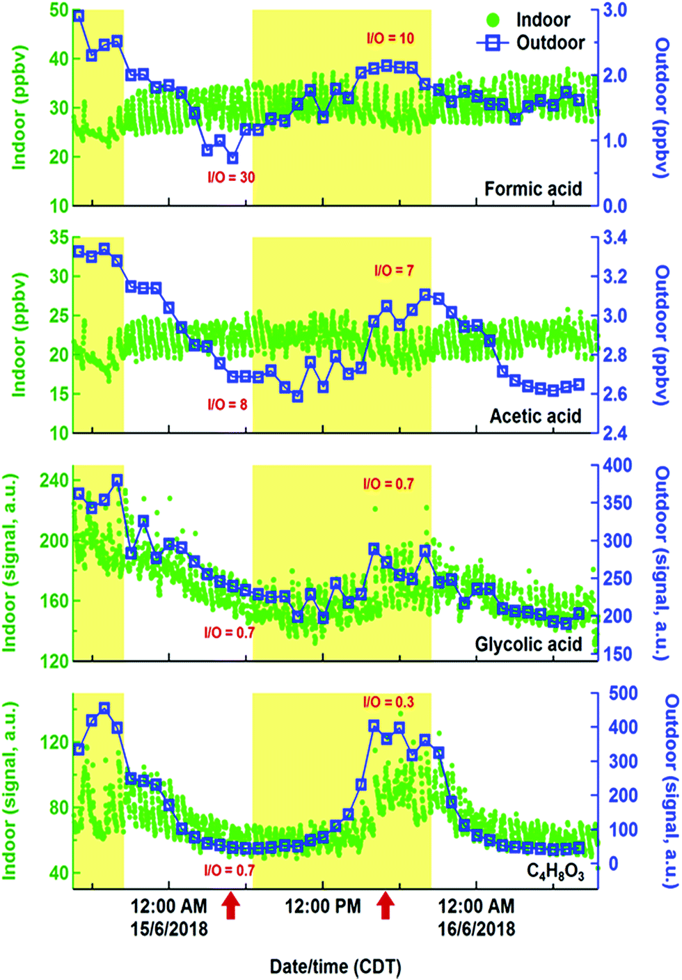 | ||
| Fig. 9 Time series of indoor (green markers) and outdoor (blue lines and markers) iodide CIMS measurements of formic acid, acetic acid, glycolic acid, and C4H8O3 during an extensive background period. Formic and acetic acid data are calculated concentrations (part per billion by volume). Glycolic acid and C4H8O3 data are measured CIMS signal (arbitrary units). Red arrows indicate approximate times during which representative indoor-to-outdoor ratios (I/O) are evaluated (June 15 at approximately 04:30 and 16:30). Daytime (06:30–20:30) periods are indicated by yellow highlighted regions. | ||
Indoor sources of formic and acetic acid during unoccupied, unperturbed background periods include off-gassing from building materials and household products79,82 and O3-initiated reactions.79,83 As in earlier studies, our data show higher concentrations of formic and acetic acids indoors than outdoors, demonstrating the importance of indoor sources. Outdoor concentrations have little effect on indoor formic and acetic acid. In contrast to indoors, outdoor formic and acetic acid exhibit strong diel patterns during the study, consistent with previous outdoor measurements that indicate photochemical sources of these acids.77,78,84 The high (≫1) indoor/outdoor concentration ratios for formic and acetic acid are consistent with the interior of the HOMEChem building being a non-photochemical source of these two acids to the atmosphere. Assuming these acids are in steady state with indoor surfaces, we estimate an upper bound emission rate from indoors to outdoors to be 2 × 10⁻⁴ mol h−1 for formic acid and 1 × 10⁻⁴ mol h−1 for acetic acid. This calculation assumes indoor-to-outdoor transport was 100% efficient, although water soluble oxygenated VOCs can be lost to indoor surfaces.81 A test house-equivalent area of managed lawn soil would be expected to emit ∼6 × 10⁻⁵ mol h−1 of formic acid and 3–5 × 10⁻⁴ mol h−1 of acetic acid.85 Residential homes may therefore be a stronger source of formic acid to outdoor urban atmospheres than area-equivalent emissions from soil.
The building is apparently not a source of all organic acids to the outdoor atmosphere during HOMEChem. The indoor to outdoor ratio of glycolic acid and C4H8O3 (likely hydroxybutyric acid) are less than 1 (Fig. 9), consistent with an outdoor source contributing substantially to the indoor abundance. Both the outdoor and indoor diel cycles of these two acids maximize in the mid-afternoon, similar to that of O3. While the indoor-to-outdoor ratio for glycolic acid is constant through the day, ratios for C4H8O3 are suppressed during the day relative to night. This diel variation implies additional daytime sinks of C4H8O3.
The building is a source of many organic acids, but HOMEChem activities highlight a complex array of possible indoor organic acid sources. Similar to previous observations,81 all water soluble organic acids cycled rapidly throughout the day coincident with the cycling of the HVAC system, and consistent with a hypothesis that the acids are lost to condensing water on the cooling system coils with re-evaporation occurring between cooling cycles. However, a 4 day time series (June 22–25; Fig. 10) for three selected organic acids indicates additional sources and sinks. Sorbic (2,4-hexadienoic acid, C6H8O2), lactic (2-hydroxypropanoic acid, CH3CHOHCOOH) and benzoic (benzene carboxylic acid, C6H5COOH) acid were all detected by acetate CIMS. Lactic acid has both cooking (e.g. meat cooking for dinner on June 25) and human sources (e.g. increase during open house and maintenance days, June 22 and 23). Benzoic acid has only cooking sources (e.g. cooking lunch on June 25), consistent with its use as a food preservative. Sorbic acid displays a more complex pattern. It is a food preservative and an ingredient in personal care products and cosmetics, and shows clear enhancements during cooking events on the layered day, June 25 (Fig. 10). Personal care products correspond to elevated sorbic acid on the Open House day (June 22), but not on the staggered occupancy day (June 24), which experienced fewer individuals in the house (e.g. a maximum of 12 versus 40+ individuals present during the Open House). We observe a decline in sorbic acid mixing ratio throughout the open house day, consistent with its possible presence in personal care products applied in the morning with diminishing signals as the day progresses, as has been previously reported for the siloxane, D5, widely used in antiperspirants.7
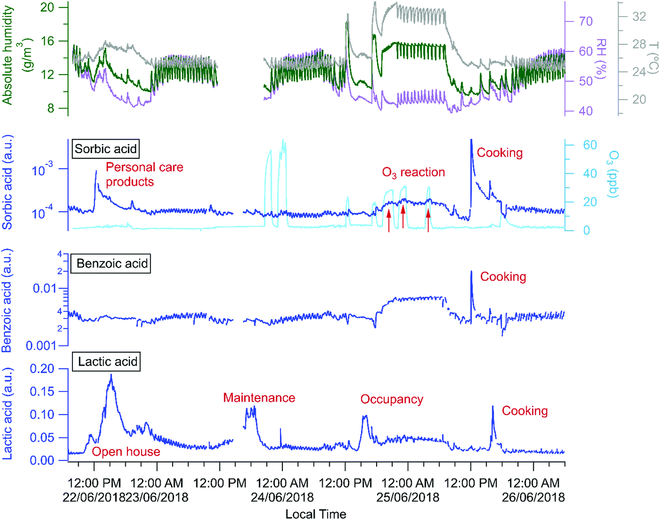 | ||
| Fig. 10 Three organic acids – sorbic, benzoic, and lactic acid – varied during four days of the campaign (open house, maintenance, occupancy, and layered day) with temperature in grey, relative humidity/RH in purple, and absolute humidity/AH in dark green. Cooking or food sources of all three organic acids are apparent, as are occupant emissions of lactic acid and personal care product sources of sorbic acid. | ||
Relative to other unoccupied evenings (e.g. night of June 22 or 26), all three acids (sorbic, lactic, and benzoic) were present at elevated concentrations on the night of June 24–25. Although this elevated acid signal coincided with O3 addition experiments, we speculate that the increased signals are more likely due to higher temperatures in the house that enable shifts in partitioning from indoor surfaces and aerosol particles to indoor air. However, we observed additional increase of sorbic acid signal that overlaps with the O3 addition periods (indicated by the red arrows in Fig. 10), suggesting that sorbic acid may be an indoor ozonolysis reaction product and that secondary chemistry influences indoor organic acid concentrations – but only under elevated ozone conditions.
3.4 Case study 4: deposition on indoor surfaces
Surfaces play important roles in the lifetime and reactivity of indoor pollutant emissions.13,86,87 Trace gases and particles can deposit to surfaces, potentially persisting for extended periods if unperturbed.88 Surface deposited material can undergo reactions on much longer timescales than indoor air reactions, which are typically limited to hours by the time scale of building air exchange. Organic films on surfaces can also alter chemical and physical properties at the air-surface interface.89,90 Surface samples were collected during HOMEChem, and here we describe initial results aimed at understanding the chemical, physical and morphological state of surface-bound species.Deposited particles were collected on vertically-mounted pieces of window glass. Analyses are presented in detail in ESI Section S2.† As expected, the surfaces collected more particles across the entire submicron size range during stir-fry events (equivalent average film growth rate of 0.09 ± 0.05 nm h−1, though only a small fraction of the glass surface was covered with particles) compared to unoccupied periods (thickness growth rate of 0.02 ± 0.03 nm h−1). Consistent with measured aerosol size distributions, many deposited particles were ultrafine (<100 nm), with a peak in the number versus volume equivalent diameter at approximately 20 nm in diameter (Fig. S8†). The predominance of ultrafine particle deposition on window glass is consistent with previous studies of kitchen activities.91–93
We probed the surface-bound particles with atomic force microscopy coupled to infrared imaging (AFM-IR). Fig. 11 shows the 3-D height image and line profile for a single particle deposited on window glass from a stir-fry event along with the infrared spectra collected across the particle at the corresponding marked location. These spectral features suggest that the particle is largely comprised of carboxylate containing organics, as shown by the peaks at around 1570 and 1430 cm−1 associated with the asymmetric (νas) and symmetric (νs) stretching vibration modes for carboxylate.94 The detection of carboxylate groups is consistent with deposition of fatty acids emitted during the stir fry process91 – and with the aerosol mass spectra discussed in the cooking case study (§3.2). The absence of the vibrational mode at 1700 cm−1 associated with the C![[double bond, length as m-dash]](https://www.rsc.org/images/entities/char_e001.gif) O stretch for protonated carboxylic acid groups suggests either deprotonation of the fatty acid-rich particles via binding between the carboxylate group with the silica and metal ions from the window glass, or that the surface film is alkaline in nature leading to the presence of deprotonated carboxylate groups.
O stretch for protonated carboxylic acid groups suggests either deprotonation of the fatty acid-rich particles via binding between the carboxylate group with the silica and metal ions from the window glass, or that the surface film is alkaline in nature leading to the presence of deprotonated carboxylate groups.
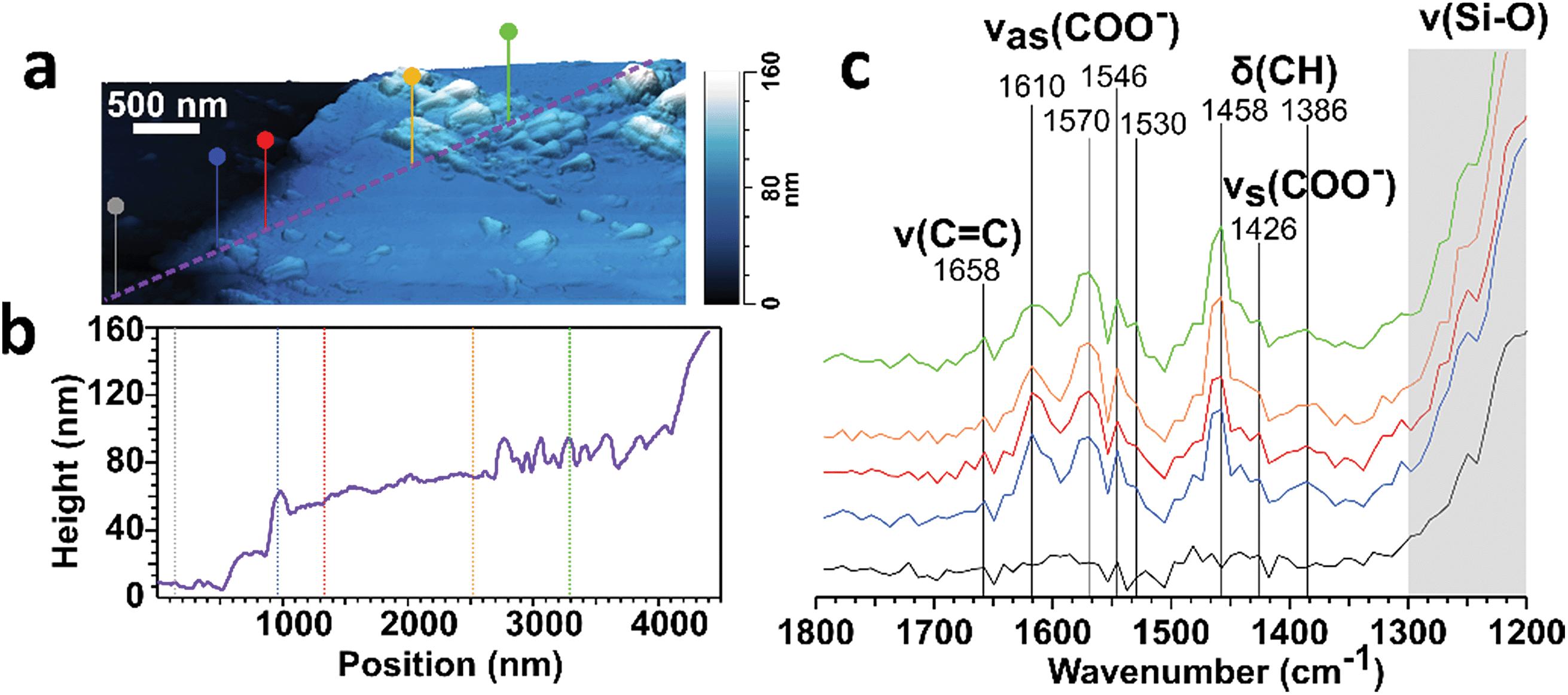 | ||
| Fig. 11 (a) 3-D AFM height image of a deposition on window glass from a stir-fry event. (b) Height profile from the purple line shown in panel (a). and (c) IR spectra taken at the corresponding colored markers in panels A and B. | ||
Surface depositions were also extracted from multiple glass surfaces and analyzed for bulk composition using an array of techniques. In contrast to previous longer-term studies of glass exposed for 3 to 6 months,88 inductively-coupled plasma mass spectrometry (ICP-MS) detected little difference in elemental composition of surface depositions from the unoccupied background, cooking (shakedown day), and stir-fry samples. Compared to the unoccupied background, only iron and magnesium showed significant enrichment in the shakedown (50% increase) and stir-fry sample (31% increase), respectively (Fig. S9 and Table S1†). The lack of differentiation in surface deposition of metals suggests relatively low levels of metal emissions during cooking, in addition to smaller sample size and decreased exposure durations in comparison to previous work. Relatively high background levels are attributable to metals in window glass leaching into the extraction solvent.
The similarity between organic molecules accumulated on surfaces and the lower volatility material present in aerosol particles is apparent from a direct comparison of deposited material and indoor and outdoor aerosol samples. In a separate set of samples from the ones discussed above, two large glass surfaces were mounted vertically above the stove for the duration of the campaign. Solvent extractions utilized a custom-built indoor surface extractor with acetonitrile. In addition to the surface samples, two different filters collected aerosol particles indoors and outdoors for the duration of the campaign, and were also extracted by acetonitrile solvent. The chemical composition of the water soluble fraction of these surface and aerosol filter extracts was analyzed by HR-AMS following atomization by a Small Volume Nebulizer.50 This analysis approach enables a comparison of ensemble properties of the organic material on surfaces and in aerosol particles.
The signal intensities of the mass spectra for the indoor aerosol filter and surface extracts have high overlap, with a dot product of 0.98 (Fig. 12a). In contrast, mass spectra of surface extracts and outdoor aerosol show less overlap (dot product of 0.86, Fig. 12b). The similar chemical composition between the indoor aerosol filter and the organic matter deposited near the stove indicates that indoor generated aerosol is the dominant source of these surface deposits. The indoor aerosol is less oxidized than the outdoor sample, with an average O/C of 0.21 indoors versus 0.30 outdoors. The outdoor aerosol sample also has more nitrogen containing organic ions compared to the indoor aerosol and surface samples. Differences between the campaign-averaged surface extracts and indoor aerosol are small, with slightly lower H/C ratios on the surface. The examples presented in this case study demonstrate advances in analytical techniques to better understand the chemical and physical properties of material deposited on indoor surfaces.
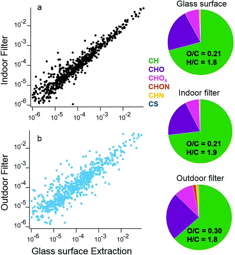 | ||
| Fig. 12 Off-line AMS measurements of extracts from filters sampling indoors and outdoors for the full campaign are compared to extracted surface depositions from a glass surface deployed above the stove during the campaign. The intensities of each peak in the mass spectra are compared for surface extracts and (a) the indoor aerosol filter or (b) the outdoor aerosol filter. The pie charts on the right show the mass fractions of different ion types for the glass surface, indoor aerosol filter, and outdoor aerosol filter. | ||
3.5 Case study 5: intercomparison of NO2 measurements
The HOMEChem study design intentionally measured the same gas and particle analytes by multiple instruments (Tables 1–4). This approach not only ensured data coverage in the event of instrument problems, but also provided opportunities for measurement intercomparisons in the indoor environment. Several observations were as expected. For example, ultrafine particles initially provided spurious signal in the UV absorption O3 detector,95 but filters placed on inlets minimized this interference. Nitrogen dioxide provides a useful case study for instrument intercomparisons: despite their prevalence in air pollution monitoring, the outdoor atmospheric chemistry community has long noted interferences in some of the most commonly used NO2 detection techniques.58 Here, we compare NO2 detected indirectly by the blue light converter coupled to chemiluminescence NO detection (hereafter BLC-NO2) compared to NO2 detected directly by cavity attenuated phase-shift spectroscopy (CAPS) (hereafter CAPS-NO2). The BLC and CAPS detector inlets were located adjacent to each other. Differences in time averaging – namely the slower time resolution of the BLC detector – account for some of the suppressed BLC-NO2 measurements during rapid events. However, even accounting for these distinctions, discrepancies between the two measurement systems persist.During intensive cooking events, BLC-NO2 provides strong negative readings – as low as −853 ppb during the Thanksgiving event of 18 June. We attribute these negative values for BLC-NO2 to VOC interferences in the photolysis cell. Molecules like glyoxal can produce HO2 upon photolysis by blue light that converts NO to NO2. The resulting HO2 suppresses the NO in the detected NO + NO2 total from the blue light converter, resulting in a NOx signal that is smaller than NO, and thus a negative NO2 if ambient NO is greater than ambient NO2. The HOMEChem Thanksgiving observations are consistent with this inferred interference: at 15:45 on 18 June, NO is 965 ppb, while NO2 is reported as −853 ppb (Fig. 13c). Thus, there is enough RO2 or HO2 formed within the blue light converter to transform almost all of the NO to NO2 and outcompete simultaneous NO2 photolysis. The result is only 112 ppb NO entering the chemiluminescence detector from the blue light converter during NOx detection mode. The negative BLC-NO2 implies that substantial RO2-producing (i.e. photolabile) VOCs are present indoors during the Thanksgiving experiments. This observation is consistent with elevated levels of organic molecules including peroxide, carboxylic acid and carbonyl moieties. If such photolabile molecules move from indoor air to the outdoor atmosphere, they may contribute to urban outdoor radical budgets.
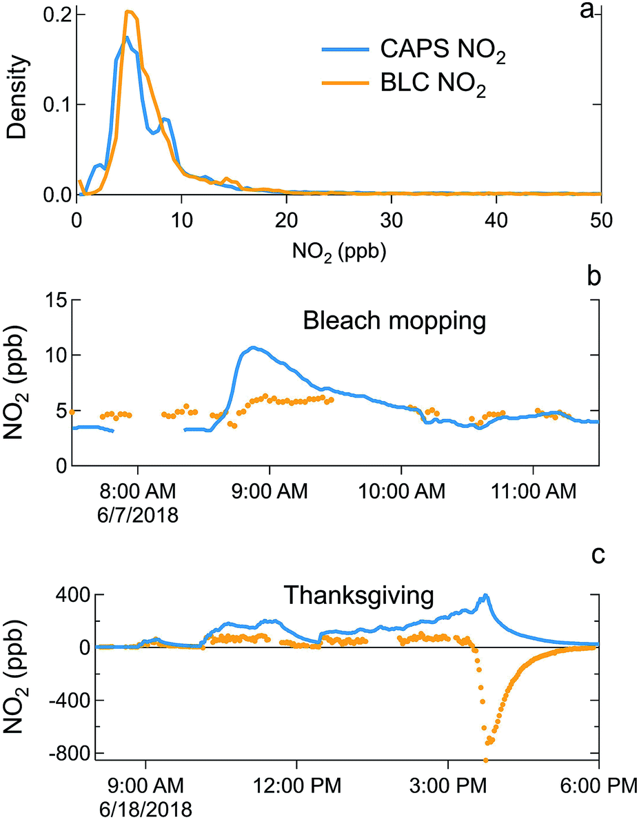 | ||
| Fig. 13 Normalized probability distributions of background indoor NO2 (a) demonstrates that NO2 detected by the CAPS (CAPS-NO2, blue) is slightly lower than the blue-light converter (BLC-NO2, orange). (b) CAPS-NO2 is enhanced during bleach mopping events, while BLC-NO2 does not change substantially during bleach mopping. (c) BLC-NO2 is subject to negative interferences during intensive cooking events, including Thanksgiving. Breaks in the BLC-NO2 timeseries occur when the sampling manifold switched to outdoor air (excluded from this figure). | ||
In addition to Thanksgiving, BLC-NO2 was also negative at the end of each layered day when NOx was elevated above background from cooking and volunteers mopped with bleach before exiting the test house. This negative BLC-NO2 suggests that chlorine chemistry is a source of radicals that react with NOx under blue light, potentially through the production of HO2 or RO2 radicals.
During sequential chlorine bleach mopping, the CAPS-NO2 signal increased above background concentrations, while the BLC-NO2 remained stable or even slightly suppressed. These simultaneous yet opposite trends in CAPS-NO2 and BLC-NO2 occurred in the absence of NOx addition from cooking on both sequential bleach mopping days (7 and 10 June) (Fig. 13b). These intercomparison deviations may be the result of a negative interference in BLC-NO2 from NO reactions in the photolytic converter, or possibly a positive interference in CAPS-NO2 from chlorinated species.
The BLC detector consistently detects higher background of unperturbed NO2 inside the house than the CAPS detector (Fig. 13a). This systematic difference may be due to different background and calibration approaches between the two systems. Removing all data points in which the relative error of BLC-NO2 (σBLC NO2/[NO2] × 100%) is below 0 or above 50% identifies the cooking interferences described above. However, once these points are removed, we still observe a persistent bias causing CAPS-NO2 to be higher than BLC-NO2 (r2 = 0.69, slope 2.16 ± 0.01), even when chlorine bleach cleaning events are removed. The histogram of the difference between CAPS-NO2 and BLC-NO2 follows a Gaussian distribution with a mean difference of 0.6 ppb and a standard deviation of 1.3 ppb, consistent with an offset in the instrument calibrations and background. However, restricting the analysis further to unperturbed house conditions only (i.e. when CAPS-NO2 < 10 ppb and BLC-NO2 > 0 ppb) results in a slope of 0.99 ± 0.01. Thus, the two instruments agree well under low-NO2, unperturbed conditions. Under these unperturbed, low-NOx conditions, the correlation coefficient between the two timeseries is low (r2 of 0.55), but this outcome may be due to limits on the relative precision of the instruments. This instrument intercomparison highlights the need for overlapping measurements of even commercially available or simpler instrumentation, particularly when intended for use in indoor environments.
4. Conclusions
The HOMEChem field campaign represents coordinated deployment of a particularly large assemblage of indoor air and surface measurement capabilities applied to simulated real-life conditions in a full-sized test house. The case studies described here illustrate several aspects of human influence on trace gas and particle composition of residential air through direct emissions, use of commercial products, and occupant activities. The research has focused on everyday activities performed in home environments (i.e. cooking, cleaning, and human occupancy). The study also offers the opportunity to contrast indoor and outdoor background air in a residential test house.Background air is generally lower in particle concentration indoors than outdoors. During cooking events, large enhancements in particle mass occur, with a substantial fraction of these increases due to chemical species related to cooking oils. By number, these cooking-associated particles are predominantly in the ultrafine mode, but substantial mass changes are observed in the accumulation and super-micron modes. The emitted particles remain in indoor air for short periods relative to persistence time scales in the outdoor atmosphere. Indoor emitted particles also evolve chemically throughout the cooking processes, with particles becoming slightly more oxygenated and nitrogenated when food is added to cooking oil. The chemical signature of cooking aerosol is observed in the organic molecules deposited on surfaces, as evidenced through both mass spectrometry and spectroscopic techniques. The large amount of organic material deposited on indoor surfaces can interact with the surface itself, as evidenced by the AFM-IR results.
Cooking also generates gas phase emissions, including hydrocarbons and more complex oxidized organic molecules, such as sorbic and lactic acid. Even in the absence of cooking or other perturbations, gas phase organics were generally higher indoors than outdoors across a broad range of species. Indoor concentrations of formic and acetic acid during HOMEChem were consistent with levels reported in previous studies. Persistently high concentrations of organic acids indoors suggest that buildings themselves may be sources of these compounds to outdoor air.
HOMEChem highlights the opportunities for new measurement techniques, including real-time high resolution time-of-flight mass spectrometry and surface measurements, for investigating the complex influences of buildings, occupants, and their activities on indoor chemistry. The instrument intercomparisons also highlight some new challenges in indoor chemistry research: the vast array of previously unmeasured and unexpected compounds that are clearly present indoors can complicate measurements and thus interpretation of chemical data. The HOMEChem dataset is, in itself, a promising demonstration of the usefulness of open-access experimental data to the indoor air quality community as well-curated and archived datasets can be used by researchers from a variety of fields, such as chemists, engineers, exposure scientists, and toxicologists to model chemical reactions, estimate exposure levels, and develop appropriate risk management strategies, among many other possibilities.
Data availability
All final data from the HOMEChem project will be available in the ICARTT format to other researchers within two years of the conclusion of the field measurements (i.e. by July 1, 2020).Conflicts of interest
There are no conflicts to declare.Acknowledgements
We thank the entire HOMEChem science team of faculty, researchers, and students, over 60 members in total, for operating instruments, volunteering for activities, and contributing to experimental design. We thank the Alfred P. Sloan Foundation for funding the HOMEChem experiment and analysis (G-2017-9944; G-2017-9692; G-2016-7049; G-2016-7050, G-2018-11062; G-2018-11031; G-2018-10128; G-2018-11366; G-2018-11035, G-2016-7173). JLJ also acknowledges funding from the CIRES Innovative Research Program. Dr Manabu Shiraiwa, Dr Glenn Morrison and the MOCCIE group provided input on experimental design. We acknowledge the Novoselac research group for preparing and operating the test house, the UT Austin CEER staff for logistical support, and the UT Austin Pickle Research Campus for hosting the research project. REO thanks Jesse H. Kroll at MIT for the use of his HR-ToF-AMS for off-line AMS data collection.References
- N. E. Klepeis, W. C. Nelson, W. R. Ott, J. P. Robinson, A. M. Tsang, P. Switzer, J. V. Behar, S. C. Hern and W. H. Engelmann, The National Human Activity Pattern Survey (NHAPS): A resource for assessing exposure to environmental pollutants, J. Exposure Anal. Environ. Epidemiol., 2001, 11, 231–252 CrossRef CAS PubMed.
- K. Koehler, N. Good, A. Wilson, A. Mölter, B. F. Moore, T. Carpenter, J. L. Peel and J. Volckens, The Fort Collins commuter study: Variability in personal exposure to air pollutants by microenvironment, Indoor Air, 2019, 29, 231–241 CrossRef CAS PubMed.
- D. Campagnolo, D. E. Saraga, A. Cattaneo, A. Spinazze, C. Mandin, R. Mabilia, E. Perreca, I. Sakellaris, N. Canha, V. G. Mihucz, T. Szigeti, G. Ventura, J. Madureira, E. D. Fernandes, Y. de Kluizenaar, E. Cornelissen, O. Hanninen, P. Carrer, P. Wolkoff, D. M. Cavallo and J. G. Bartzis, VOCs and aldehydes source identification in European office buildings - The OFFICAIR study, Building and Environment, 2017, 115, 18–24 CrossRef.
- Y. Liu, P. K. Misztal, J. Xiong, Y. Tian, C. Arata, R. J. Weber, W. W. Nazaroff and A. H. Goldstein, Characterizing sources and emissions of volatile organic compounds in a northern California residence using space-and time-resolved measurements, Indoor Air, 2019, 29(4), 630–644, DOI:10.1111/ina.12562.
- J. P. S. Wong, N. Carslaw, R. Zhao, S. Zhou and J. P. D. Abbatt, Observations and impacts of bleach washing on indoor chlorine chemistry, Indoor Air, 2017, 27, 1082–1090 CrossRef CAS PubMed.
- A. C. Steinemann, I. C. MacGregor, S. M. Gordon, L. G. Gallagher, A. L. Davis, D. S. Ribeiro and L. A. Wallace, Fragranced consumer products: Chemicals emitted, ingredients unlisted, Environmental Impact Assessment Review, 2011, 31, 328–333 CrossRef.
- X. Tang, P. K. Misztal, W. W. Nazaroff and A. H. Goldstein, Siloxanes are the most abundant volatile organic compound emitted from engineering students in a classroom, Environ. Sci. Technol. Lett., 2015, 2, 303–307 CrossRef CAS.
- P. K. Misztal, D. S. Lymperopoulou, R. I. Adams, R. A. Scott, S. E. Lindow, T. Bruns, J. W. Taylor, J. Uehling, G. Bonito, R. Vilgalys and A. H. Goldstein, Emission factors of microbial volatile organic compounds from environmental bacteria and fungi, Environ. Sci. Technol., 2018, 52, 8272–8282 CrossRef CAS PubMed.
- J. Williams, C. Stönner, J. Wicker, N. Krauter, B. Derstroff, E. Bourtsoukidis, T. Klüpfel and S. Kramer, Cinema audiences reproducibly vary the chemical composition of air during films, by broadcasting scene specific emissions on breath, Sci. Rep., 2016, 6, 25464 CrossRef CAS PubMed.
- L. A. Wallace, S. J. Emmerich and C. Howard-Reed, Source strengths of ultrafine and fine particles due to cooking with a gas stove, Environ. Sci. Technol., 2004, 38(8), 2304–2311 CrossRef CAS PubMed.
- K. Kristensen, D. M. Lunderberg, Y. Liu, P. K. Misztal, Y. Tian, C. Arata, W. W. Nazaroff and A. H. Goldstein, Sources and dynamics of semivolatile organic compounds in a single-family residence in Northern California, Indoor Air, 2019, 29(4), 645–655, DOI:10.1111/ina.12561.
- G. Morrison, Interfacial chemistry in indoor environments, Environ. Sci. Technol., 2008, 42, 3494–3499 CrossRef CAS PubMed.
- C. J. Weschler and N. Carslaw, Indoor chemistry, Environ. Sci. Technol., 2018, 52, 2419–2428 CrossRef CAS PubMed.
- N. Carslaw, A new detailed chemical model for indoor air pollution, Atmos. Environ., 2007, 41, 1164–1179 CrossRef CAS.
- M. M. Coggon, B. C. McDonald, A. Vlasenko, P. R. Veres, F. Bernard, A. R. Koss, B. Yuan, J. B. Gilman, J. Peischl, K. C. Aikin, J. DuRant, C. Warneke, S. M. Li and J. A. de Gouw, Diurnal variability and emission pattern of decamethylcyclopentasiloxane (D-5) from the application of personal care products in two North American cities, Environ. Sci. Technol., 2018, 52, 5610–5618 CrossRef CAS PubMed.
- B. C. McDonald, J. A. de Gouw, J. B. Gilman, S. H. Jathar, A. Akherati, C. D. Cappa, J. L. Jimenez, J. Lee-Taylor, P. L. Hayes, S. A. McKeen, Y. Y. Cui, S. W. Kim, D. R. Gentner, G. Isaacman-VanWertz, A. H. Goldstein, R. A. Harley, G. J. Frost, J. M. Roberts, T. B. Ryerson and M. Trainer, Volatile chemical products emerging as largest petrochemical source of urban organic emissions, Science, 2018, 359, 760–764 CrossRef CAS PubMed.
- D. K. Farmer and J. L. Jimenez, Real-time atmospheric chemistry field instrumentation, Anal. Chem., 2010, 82(19), 7879–7884, DOI:10.1021/ac1010603.
- D. K. Farmer, Analytical challenges and opportunities for indoor air chemistry field studies, Anal. Chem., 2019, 91, 3761–3767 CrossRef CAS PubMed.
- C. Arata, K. J. Zarzana, P. K. Misztal, Y. J. Liu, S. S. Brown, W. W. Nazaroff and A. H. Goldstein, Measurement of NO3 and N2O5 in a Residential Kitchen, Environ. Sci. Technol. Lett., 2018, 5, 595–599 CrossRef CAS.
- D. B. Collins, R. F. Hems, S. M. Zhou, C. Wang, E. Grignon, M. Alavy, J. A. Siegel and J. P. D. Abbatt, Evidence for gas-surface equilibrium control of indoor nitrous acid, Environ. Sci. Technol., 2018, 52, 12419–12427 CrossRef CAS PubMed.
- S. F. Kowal, S. R. Allen and T. F. Kahan, Wavelength-resolved photon fluxes of indoor light sources: Implications for HOx production, Environ. Sci. Technol., 2017, 51, 10423–10430 CrossRef CAS PubMed.
- A. M. Avery, M. S. Waring and P. F. DeCarlo, Human occupant contribution to secondary aerosol mass in the indoor environment, Environ. Sci.: Processes Impacts, 2019 10.1039/C9EM00097F.
- P. F. DeCarlo, A. M. Avery and M. S. Waring, Thirdhand smoke uptake to aerosol particles in the indoor environment, Sci. Adv., 2018, 4, eaap8368, DOI:10.1126/sciadv.aap8368.
- P. L. Kebabian, E. C. Wood, S. C. Herndon and A. Freedman, A practical alternative to chemiluminescence-based detection of nitrogen dioxide: Cavity attenuated phase shift spectroscopy, Environ. Sci. Technol., 2008, 42, 6040–6045 CrossRef CAS PubMed.
- S. Dusanter, D. Vimal and P. S. Stevens, Technical note: Measuring tropospheric OH and HO2 by laser-induced fluorescence at low pressure. A comparison of calibration techniques, Atmos. Chem. Phys., 2008, 8, 321–340 CrossRef CAS.
- S. Dusanter, D. Vimal, P. S. Stevens, R. Volkamer, L. T. Molina, A. Baker, S. Meinardi, D. Blake, P. Sheehy, A. Merten, R. Zhang, J. Zheng, E. C. Fortner, W. Junkermann, M. Dubey, T. Rahn, B. Eichinger, P. Lewandowski, J. Prueger and H. Holder, Measurements of OH and HO2 concentrations during the MCMA-2006 field campaign - Part 2: Model comparison and radical budget, Atmos. Chem. Phys., 2009, 9, 6655–6675 CrossRef CAS.
- M. M. Lew, S. Dusanter and P. S. Stevens, Measurement of interferences associated with the detection of the hydroperoxy radical in the atmosphere using laser-induced fluorescence, Atmos. Meas. Tech., 2018, 11, 95–109 CrossRef.
- A. Abeleira, I. B. Pollack, B. Sive, Y. Zhou, E. V. Fischer and D. K. Farmer, Source characterization of volatile organic compounds in the Colorado Northern Front Range Metropolitan Area during spring and summer 2015, J. Geophys. Res.: Atmos., 2017, 122, 3595–3613 Search PubMed.
- X. Tang, P. K. Misztal, W. W. Nazaroff and A. H. Goldstein, Volatile organic compound emissions from humans indoors, Environ. Sci. Technol., 2016, 50, 12686–12694 CrossRef CAS PubMed.
- P. Brophy and D. K. Farmer, A switchable reagent ion high resolution time-of-flight chemical ionization mass spectrometer for real-time measurement of gas phase oxidized species: characterization from the 2013 southern oxidant and aerosol study, Atmos. Meas. Tech., 2015, 8, 2945–2959 CrossRef CAS.
- J. M. Roberts, P. Veres, C. Warneke, J. A. Neuman, R. A. Washenfelder, S. S. Brown, M. Baasandorj, J. B. Burkholder, I. R. Burling, T. J. Johnson, R. J. Yokelson and J. de Gouw, Measurement of HONO, HNCO, and other inorganic acids by negative-ion proton-transfer chemical-ionization mass spectrometry (NI-PT-CIMS): application to biomass burning emissions, Atmos. Meas. Tech., 2010, 3, 981–990 CrossRef CAS.
- R. F. Hems, C. Wang, D. B. Collins, S. Zhou, N. Borduas-Dedekind, J. A. Siegel and J. P. D. Abbatt, Sources of isocyanic acid (HNCO) indoors: a focus on cigarette smoke, Environ. Sci.: Processes Impacts, 2019 10.1039/C9EM00107G.
- F. D. Lopez-Hilfiker, C. Mohr, M. Ehn, F. Rubach, E. Kleist, J. Wildt, T. F. Mentel, A. Lutz, M. Hallquist, D. Worsnop and J. A. Thornton, A novel method for online analysis of gas and particle composition: description and evaluation of a Filter Inlet for Gases and AEROsols (FIGAERO), Atmos. Meas. Tech., 2014, 7, 983–1001 CrossRef.
- G. Isaacman, N. M. Kreisberg, L. D. Yee, D. R. Worton, A. W. H. Chan, J. A. Moss, S. V. Hering and A. H. Goldstein, Online derivatization for hourly measurements of gas- and particle-phase semi-volatile oxygenated organic compounds by thermal desorption aerosol gas chromatography (SV-TAG), Atmos. Meas. Tech., 2014, 7, 4417–4429 CrossRef.
- P. F. DeCarlo, J. R. Kimmel, A. Trimborn, M. J. Northway, J. T. Jayne, A. C. Aiken, M. Gonin, K. Fuhrer, T. Horvath, K. S. Docherty, D. R. Worsnop and J. L. Jimenez, Field-deployable, high-resolution, time-of-flight aerosol mass spectrometer, Anal. Chem., 2006, 78, 8281–8289 CrossRef CAS PubMed.
- R. Fröhlich, M. J. Cubison, J. G. Slowik, N. Bukowiecki, A. S. H. Prévôt, U. Baltensperger, J. Schneider, J. R. Kimmel, M. Gonin, U. Rohner, D. R. Worsnop and J. T. Jayne, The ToF-ACSM: a portable aerosol chemical speciation monitor with TOFMS detection, Atmos. Meas. Tech., 2013, 6, 3225–3241 CrossRef.
- N. L. Ng, S. C. Herndon, A. Trimborn, M. R. Canagaratna, P. L. Croteau, T. B. Onasch, D. Sueper, D. R. Worsnop, Q. Zhang, Y. L. Sun and J. T. Jayne, An Aerosol Chemical Speciation Monitor (ACSM) for routine monitoring of the composition and mass concentrations of ambient aerosol, Aerosol Sci. Technol., 2011, 45, 780–794 CrossRef CAS.
- J. Cai, B. Yan, J. Ross, D. Zhang, P. L. Kinney, M. S. Perzanowski, K. Jung, R. Miller and S. N. Chillrud, Validation of MicroAeth® as a black carbon monitor for fixed-site measurement and optimization for personal exposure characterization, Aerosol Air Qual. Res., 2014, 14, 1–9 CrossRef CAS PubMed.
- L. Drinovec, G. Mocnik, P. Zotter, A. S. H. Prévôt, C. Ruckstuhl, E. Coz, M. Rupakheti, J. Sciare, T. Muller, A. Wiedensohler and A. D. A. Hansen, The “dual-spot” Aethalometer: an improved measurement of aerosol black carbon with real-time loading compensation, Atmos. Meas. Tech., 2015, 8, 1965–1979 CrossRef CAS.
- P. K. Diwakar and P. Kulkarni, Measurement of elemental concentration of aerosols using spark emission spectroscopy, J. Anal. At. Spectrom., 2012, 27, 1101–1109 RSC.
- J. Kangasluoma, A. Franchin, J. Duplissy, L. Ahonen, F. Korhonen, M. Attoui, J. Mikkilä, K. Lehtipalo, J. Vanhanen, M. Kulmala and T. Petäjä, Operation of the Airmodus A11 nano Condensation Nucleus Counter at various inlet pressures and various operation temperatures, and design of a new inlet system, Atmos. Meas. Tech., 2016, 9, 2977–2988 CrossRef CAS.
- R. S. Gao, H. Telg, R. J. McLaughlin, S. J. Ciciora, L. A. Watts, M. S. Richardson, J. P. Schwarz, A. E. Perring, T. D. Thornberry, A. W. Rollins, M. Z. Markovic, T. S. Bates, J. E. Johnson and D. W. Fahey, A light-weight, high-sensitivity particle spectrometer for PM2.5 aerosol measurements, Aerosol Sci. Technol., 2016, 50, 88–99 CrossRef CAS.
- Y. Cai, D. C. Montague, W. Mooiweer-Bryan and T. Deshler, Performance characteristics of the ultra high sensitivity aerosol spectrometer for particles between 55 and 800 nm: Laboratory and field studies, J. Aerosol Sci., 2008, 39, 759–769 CrossRef CAS.
- B. T. Chen, Y. S. Cheng and H. C. Yeh, Performance of a TSI aerodynamic particle sizer, Aerosol Sci. Technol., 1985, 4, 89–97 CrossRef.
- V. Agranovski, Z. Ristovski, M. Hargreaves, P. J. Blackall and L. Morawska, Real-time measurement of bacterial aerosols with the UVAPS: performance evaluation, J. Aerosol Sci., 2003, 34, 301–317 CrossRef CAS.
- I. Protsyuk, A. V. Melnik, L. F. Nothias, L. Rappez, P. Phapale, A. A. Aksenov, A. Bouslimani, S. Ryazanov, P. C. Dorrestein and T. Alexandrov, 3D molecular cartography using LC-MS facilitated by Optimus and 'ili software, Nat. Protoc., 2018, 13, 134–154 CrossRef CAS PubMed.
- A. P. Ranney and P. J. Ziemann, Microscale spectrophotometric methods for quantification of functional groups in oxidized organic aerosol, Aerosol Sci. Technol., 2016, 50, 881–892 CrossRef CAS.
- P. C. Mouli, S. V. Mohan, V. Balaram, M. P. Kumar and S. J. Reddy, A study on trace elemental composition of atmospheric aerosols at a semi-arid urban site using ICP-MS technique, Atmos. Environ., 2006, 40, 136–146 CrossRef.
- K. Suzuki, Characterisation of airborne particulates and associated trace metals deposited on tree bark by ICP-OES, ICP-MS, SEM-EDX and laser ablation ICP-MS, Atmos. Environ., 2006, 40, 2626–2634 CrossRef CAS.
- R. E. O'Brien, K. J. Ridley, M. R. Canagaratna, J. T. Jayne, P. L. Croteau, D. R. Worsnop, S. H. Budisulistiorini, J. D. Surratt, C. L. Follett, D. J. Repeta and J. H. Kroll, Ultrasonic nebulization for the elemental analysis of microgram-level samples with offline aerosol mass spectrometry, Atmos. Meas. Tech., 2019, 12, 1659–1671 CrossRef.
- C. J. Weschler, H. C. Shields and D. V. Naik, Indoor ozone exposures, JAPCA, 1989, 39, 1562–1568 CrossRef CAS PubMed.
- C. J. Weschler, Ozone in indoor environments: Concentration and chemistry, Indoor Air, 2000, 10, 269–288 CrossRef CAS PubMed.
- J. R. Girman, M. G. Apte, G. W. Traynor, J. R. Allen and C. D. Hollowell, Pollutant emission rates from indoor combustion appliances and sidestream cigarette smoke, Environ. Int., 1982, 8, 213–221 CrossRef CAS.
- G. W. Traynor, D. W. Anthon and C. D. Hollowell, Technique for determining pollutant emissions from a gas-fired range, Atmos. Environ., 1982, 16, 2979–2987 CrossRef CAS.
- G. W. Traynor, J. R. Girman, M. G. Apte, J. F. Dillworth and P. D. White, Indoor air pollution due to emissions from unvented gas-fired space heaters, J. Air Pollut. Control Assoc., 1985, 35, 231–237 CrossRef CAS PubMed.
- S. S. Park, J. H. Hong, J. H. Lee, Y. J. Kim, S. Y. Cho and S. J. Kim, Investigation of nitrous acid concentration in an indoor environment using an in situ monitoring system, Atmos. Environ., 2008, 42, 6586–6596 CrossRef CAS.
- J. E. Borrazzo, J. F. Osborn, R. C. Fortmann, R. L. Keeper and C. I. Davidson, Modeling and monitoring of CO, NO and NO2 in a modern townhouse, Atmos. Environ., 1987, 21, 299–311 CrossRef CAS.
- E. J. Dunlea, S. C. Herndon, D. D. Nelson, R. M. Volkamer, F. San Martini, P. M. Sheehy, M. S. Zahniser, J. H. Shorter, J. C. Wormhoudt, B. K. Lamb, E. J. Allwine, J. S. Gaffney, N. A. Marley, M. Grutter, C. Marquez, S. Blanco, B. Cardenas, A. Retama, C. R. R. Villegas, C. E. Kolb, L. T. Molina and M. J. Molina, Evaluation of nitrogen dioxide chemiluminescence monitors in a polluted urban environment, Atmos. Chem. Phys., 2007, 7, 2691–2704 CrossRef CAS.
- S. Zhou, C. J. Young, T. C. VandenBoer, S. F. Kowal and T. F. Kahan, Time-resolved measurements of nitric oxide, nitrogen dioxide, and nitrous acid in an occupied New York home, Environ. Sci. Technol., 2018, 52, 8355–8364 CrossRef CAS PubMed.
- J. Zhang and P. J. Lioy, Ozone in residential air: Concentrations, I/O ratios, indoor chemistry, and exposures, Indoor Air, 1994, 4, 95–105 CrossRef CAS.
- K. Lee, J. Xue, A. S. Geyh, H. Ozkaynak, B. P. Leaderer, C. J. Weschler and J. D. Spengler, Nitrous acid, nitrogen dioxide, and ozone concentrations in residential environments, Environ. Health Perspect., 2002, 110, 145–150 CrossRef CAS PubMed.
- N. A. Mullen, J. Li, M. L. Russell, M. Spears, B. D. Less and B. C. Singer, Results of the California Healthy Homes Indoor Air Quality Study of 2011-2013: impact of natural gas appliances on air pollutant concentrations, Indoor Air, 2016, 26, 231–245 CrossRef CAS PubMed.
- D. W. Dockery and J. D. Spengler, Indoor-outdoor relationships of respirable sulfates and particles, Atmos. Environ., 1981, 15, 335–343 CrossRef CAS.
- S. Madronich, Implications of recent total atmospheric ozone measurements for biologically active ultraviolet radiation reaching the Earth's surface, Geophys. Res. Lett., 1992, 19, 37–40 CrossRef CAS.
- B. Just, S. Rogak and M. Kandlikar, Characterization of ultrafine particulate matter from traditional and improved biomass cookstoves, Environ. Sci. Technol., 2013, 47, 3506–3512 CrossRef CAS PubMed.
- A. Leavey, S. Patel, R. Martinez, D. Mitroo, C. Fortenberry, M. Walker, B. Williams and P. Biswas, Organic and inorganic speciation of particulate matter formed during different combustion phases in an improved cookstove, Environ. Res., 2017, 158, 33–42 CrossRef CAS PubMed.
- E. Abt, H. H. Suh, G. Allen and P. Koutrakis, Characterization of indoor particle sources: A study conducted in the metropolitan Boston area, Environ. Health Perspect., 2000, 108, 35–44 CrossRef CAS PubMed.
- C. He, L. Morawska, J. Hitchins and D. Gilbert, Contribution from indoor sources to particle number and mass concentrations in residential houses, Atmos. Environ., 2004, 38, 3405–3415 CrossRef CAS.
- L. Wallace, Indoor sources of ultrafine and accumulation mode particles: Size distributions, size-resolved concentrations, and source strengths, Aerosol Sci. Technol., 2006, 40, 348–360 CrossRef CAS.
- C. Mohr, J. A. Huffman, M. J. Cubison, A. C. Aiken, K. S. Docherty, J. R. Kimmel, I. M. Ulbrich, M. Hannigan and J. L. Jimenez, Characterization of primary organic aerosol emissions from meat cooking, trash burning, and motor vehicles with high-resolution aerosol mass spectrometry and comparison with ambient and chamber observations, Environ. Sci. Technol., 2009, 43, 2443–2449 CrossRef CAS PubMed.
- Q. Zhang, J. L. Jimenez, M. R. Canagaratna, I. M. Ulbrich, N. L. Ng, D. R. Worsnop and Y. L. Sun, Understanding atmospheric organic aerosols via factor analysis of aerosol mass spectrometry: A review, Anal. Bioanal. Chem., 2011, 401, 3045–3067 CrossRef CAS PubMed.
- C. Mohr, P. F. DeCarlo, M. F. Heringa, R. Chirico, J. G. Slowik, R. Richter, C. Reche, A. Alastuey, X. Querol, R. Seco, J. Peñuelas, J. L. Jiménez, M. Crippa, R. Zimmermann, U. Baltensperger and A. S. H. Prévôt, Identification and quantification of organic aerosol from cooking and other sources in Barcelona using aerosol mass spectrometer data, Atmos. Chem. Phys., 2012, 12, 1649–1665 CrossRef CAS.
- L. Y. He, Y. Lin, X. F. Huang, S. Guo, L. Xue, Q. Su, M. Hu, S. J. Luan and Y. H. Zhang, Characterization of high-resolution aerosol mass spectra of primary organic aerosol emissions from Chinese cooking and biomass burning, Atmos. Chem. Phys., 2010, 10, 11535–11543 CrossRef CAS.
- T. Liu, Z. Wang, X. Wang and C. K. Chan, Primary and secondary organic aerosol from heated cooking oil emissions, Atmos. Chem. Phys., 2018, 18, 11363–11374 CrossRef CAS.
- A. M. Johnson, M. S. Waring and P. F. DeCarlo, Real-time transformation of outdoor aerosol components upon transport indoors measured with aerosol mass spectrometry, Indoor Air, 2017, 27, 230–240 CrossRef CAS PubMed.
- J. D. Allan, P. I. Williams, W. T. Morgan, C. L. Martin, M. J. Flynn, J. Lee, E. Nemitz, G. J. Phillips, M. W. Gallagher and H. Coe, Contributions from transport, solid fuel burning and cooking to primary organic aerosols in two UK cities, Atmos. Chem. Phys., 2010, 10, 647–668 CrossRef CAS.
- P. R. Veres, J. M. Roberts, A. K. Cochran, J. B. Gilman, W. C. Kuster, J. S. Holloway, M. Graus, J. Flynn, B. Lefer, C. Warneke and J. de Gouw, Evidence of rapid production of organic acids in an urban air mass, Geophys. Res. Lett., 2011, 38, L17807, DOI:10.1029/2011GL048420.
- J. M. Mattila, P. Brophy, J. Kirkland, S. Hall, K. Ullmann, E. V. Fischer, S. Brown, E. McDuffie, A. Tevlin and D. K. Farmer, Tropospheric sources and sinks of gas-phase acids in the Colorado Front Range, Atmos. Chem. Phys., 2018, 18, 12315–12327 CrossRef CAS.
- R. Reiss, P. B. Ryan, S. J. Tibbetts and P. Koutrakis, Measurement of organic acids, aldehydes, and ketones in residential environments and their relation to ozone, J. Air Waste Manage. Assoc., 1995, 45, 811–822 CrossRef CAS.
- S. Liu, S. L. Thompson, H. Stark, P. J. Ziemann and J. L. Jimenez, Gas-phase carboxylic acids in a university classroom: Abundance, variability, and sources, Environ. Sci. Technol., 2017, 51, 5454–5463 CrossRef CAS PubMed.
- S. M. Duncan, S. Tomaz, G. Morrison, M. Webb, J. M. Atkin, J. D. Surratt and B. J. Turpin, Dynamics of residential water-soluble organic gases: Insights into sources and sinks, Environ. Sci. Technol., 2019, 53, 1812–1821 CrossRef CAS PubMed.
- J. N. Pitts, H. W. Biermann, E. C. Tuazon, M. Green, W. D. Long and A. M. Winer, Time-resolved identification and measurement of indoor air pollutants by spectroscopic techniques: Gaseous nitrous acid, methanol, formaldehyde and formic acid, JAPCA, 1989, 39, 1344–1347 CrossRef CAS PubMed.
- H. Destaillats, M. M. Lunden, B. C. Singer, B. K. Coleman, A. T. Hodgson, C. J. Weschler and W. W. Nazaroff, Indoor secondary pollutants from household product emissions in the presence of ozone: A bench-scale chamber study, Environ. Sci. Technol., 2006, 40, 4421–4428 CrossRef CAS PubMed.
- A. Chebbi and P. Carlier, Carboxylic acids in the troposphere, occurrence, sources, and sinks: A review, Atmos. Environ., 1996, 30, 4233–4249 CrossRef CAS.
- A. Mielnik, M. Link, J. Mattila, S. R. Fulgham and D. K. Farmer, Emission of formic and acetic acids from two Colorado soils, Environ. Sci.: Processes Impacts, 2018, 20, 1537–1545 RSC.
- C. J. Weschler, Chemistry in indoor environments: 20 years of research, Indoor Air, 2011, 21, 205–218 CrossRef CAS PubMed.
- M. Mendez, N. Blond, P. Blondeau, C. Schoemaecker and D. A. Hauglustaine, Assessment of the impact of oxidation processes on indoor air pollution using the new time-resolved INCA-Indoor model, Atmos. Environ., 2015, 122, 521–530 CrossRef CAS.
- V. W. Or, M. R. Alves, M. Wade, S. Schwab, R. L. Corsi and V. H. Grassian, Crystal clear? Microspectroscopic imaging and physicochemical characterization of indoor depositions on window glass, Environ. Sci. Technol. Lett., 2018, 5, 514–519 CrossRef CAS.
- R. Alwarda, S. Zhou and J. P. Abbatt, Heterogeneous oxidation of indoor surfaces by gas-phase hydroxyl radicals, Indoor Air, 2018, 28, 655–664 CrossRef CAS PubMed.
- M. Kruza, A. C. Lewis, G. Morrison and N. Carslaw, Impact of surface ozone interactions on indoor air chemistry: A modeling study, Indoor Air, 2017, 27, 1001–1011 CrossRef CAS PubMed.
- Y. Zhao, M. Hu, S. Slanina and Y. Zhang, The molecular distribution of fine particulate organic matter emitted from Western-style fast food cooking, Atmos. Environ., 2007, 41, 8163–8171 CrossRef CAS.
- K. L. Abdullahi, J. M. Delgado-Saborit and R. M. Harrison, Emissions and indoor concentrations of particulate matter and its specific chemical components from cooking: A review, Atmos. Environ., 2013, 71, 260–294 CrossRef CAS.
- E. Abt, H. H. Suh, P. Catalano and P. Koutrakis, Relative contribution of outdoor and indoor particle sources to indoor concentrations, Environ. Sci. Technol., 2000, 34, 3579–3587 CrossRef CAS.
- D. Lee and R. Condrate, FTIR spectral characterization of thin film coatings of oleic acid on glasses: I. Coatings on glasses from ethyl alcohol, J. Mater. Sci., 1999, 34, 139–146 CrossRef CAS.
- C. W. Spicer, D. W. Joseph and W. M. Ollison, A re-examination of ambient air ozone monitor interferences, J. Air Waste Manage. Assoc., 2010, 60, 1353–1364 CrossRef CAS.
Footnote |
| † Electronic supplementary information (ESI) available. See DOI: 10.1039/c9em00228f |
| This journal is © The Royal Society of Chemistry 2019 |