
A review of crystalline silicon bifacial photovoltaic performance characterisation and simulation
Tian Shen
Liang
 ab,
Mauro
Pravettoni
a,
Chris
Deline
c,
Joshua S.
Stein
d,
Radovan
Kopecek
e,
Jai Prakash
Singh
a,
Wei
Luo
a,
Yan
Wang
a,
Armin G.
Aberle
a and
Yong Sheng
Khoo
*a
ab,
Mauro
Pravettoni
a,
Chris
Deline
c,
Joshua S.
Stein
d,
Radovan
Kopecek
e,
Jai Prakash
Singh
a,
Wei
Luo
a,
Yan
Wang
a,
Armin G.
Aberle
a and
Yong Sheng
Khoo
*a
aSolar Energy Research Institute of Singapore (SERIS), National University of Singapore, 117574, Singapore. E-mail: yongshengkhoo@nus.edu.sg
bDepartment of Electrical and Computer Engineering, National University of Singapore, 117583, Singapore
cNational Renewable Energy Laboratory (NREL), Golden, CO 80401, USA
dSandia National Laboratories, Albuquerque, NM 87185, USA
eISC Konstanz, Konstanz 78467, Germany
First published on 19th November 2018
Abstract
Bifacial photovoltaic (PV) technology has received considerable attention in recent years due to the potential to achieve higher annual energy yield compared to its monofacial counterpart. Higher annual energy yield is a crucial factor (even more than to further reduce the module costs) because, with the use of higher power PV modules, the high BOS (Balance of System) costs can be reduced, resulting in the lowest LCOE (levelised cost of energy). The International Technology Roadmap for Photovoltaic (ITRPV) predicts an upward trend for the shares of crystalline silicon (c-Si) bifacial PV cells and modules in the global PV market in the next decade, i.e., more than 35% in 2028. Two key enabling factors have been identified to promote the widespread use of c-Si bifacial PV devices, namely the bifacial PV performance measurement method/standard for indoor characterisation and comprehensive simulation models for outdoor performance characterisation. Both will increase the bankability of bifacial PV technology. In this paper, a comprehensive review of the state-of-the-art of the c-Si bifacial PV performance characterisation and simulation is presented. First, an overview of the indoor characterisation of c-Si bifacial PV cells and modules is presented, followed by an overview of the outdoor characterisation of c-Si bifacial PV modules and the draft technical specification, IEC TS 60904-1-2. The second part of this paper reviews the current status of bifacial PV performance modelling, which includes the three primary sub-models: optical, electrical, and thermal models. This paper also provides an overview of the required future research to address the challenges associated with the characterisation and simulation of c-Si bifacial PV devices.
 Tian Shen Liang | Mr Tian Shen Liang received his BEng and MSc degrees in Mechanical Engineering from the Multimedia University, Malaysia and National University of Singapore (NUS), respectively. He also received Erasmus Mundus MSc degree in Energy Engineering from the Universitat Politècnica de Catalunya (UPC), Spain, and Royal Institute of Technology (KTH), Sweden. He is currently working as a research associate with the SERIS and doing his PhD at the Department of Electrical and Computer Engineering, NUS. His research interests include bifacial PV module performance characterisation, simulation, and optimisation. |
 Mauro Pravettoni | Dr Mauro Pravettoni obtained his PhD from the Imperial College London. He is a member of IEC and of the British Society for the Philosophy of Science. From 2007 to 2010 he was a contract agent at ESTI, the European centre of reference for PV testing. From 2010 to 2016 he was an associate researcher at SUPSI, a Swiss accredited laboratory for PV testing. Since 2017 he has been a Senior Research Fellow at SERIS, leading the module characterization team. He has written 20+ peer-reviewed papers, books, and conference proceedings. In 2008 he co-developed the world record efficiency luminescent solar concentrator. |
 Chris Deline | Dr Chris Deline received his BS, MS, and PhD degrees from the University of Michigan, Ann Arbor, in 2003, 2005, and 2008, respectively, all in electrical engineering. Since 2008 he has been a research engineer at the National Renewable Energy Laboratory in Golden, CO, in the photovoltaic performance and reliability group. He manages the US Department of Energy Regional Test Center program at NREL for field assessment of novel PV technologies and is the principal investigator for multiple PV field performance projects including degradation rate assessment and bifacial module power rating and production modelling. |
 Joshua S. Stein | Dr Joshua S. Stein is a Distinguished Member of the Technical Staff at Sandia National Laboratories where he leads PV modelling and analysis projects in support of the U.S. Department of Energy and industry partners. He develops and validates models of solar photovoltaic system performance, reliability, and grid integration. He is the founder of the PV Performance Modeling Collaborative and is an active member of the International Energy Agency PVPS Task 13 on PV Performance and Reliability. |
 Radovan Kopecek | Dr Radovan Kopecek obtained his Dipl. Phys. degree from the University of Stuttgart in 1998. In 2002 he completed his PhD dissertation in the field of c-Si thin film silicon solar cells at the University of Konstanz. One of the founders of ISC Konstanz, Dr Kopecek has been since 2007 the leader of the advanced solar cells department dealing with several European, national research projects and technology transfers focusing on high-efficiency n-type devices and bifacial technology. Since 2016 he has been in the board of directors at EUREC-European association for research centres involved in renewable R&D. |
 Yong Sheng Khoo | Dr Yong Sheng Khoo is a Senior Research Fellow at NUS and the head of the PV Module Development group at the Solar Energy Research Institute of Singapore (SERIS). Working in PV since 2010, his research includes advanced module characterization and development. In addition, he is also leading the new BIPV flagship project at SERIS. He is the lead- and co-principal investigator of multiple public grants including the Solar CRP-01 “Cost-effective high-power density Building Integrated PV (BIPV) modules”. As a recognition for his achievement in advancing PV module research, Dr Khoo received the Young Scientist Award from Singapore Minister of Environment and Water Resources in 2016. |
Broader contextThe mitigation of climate change and fulfilment of rising energy demand necessitate the adoption of photovoltaic (PV) energy. Crystalline silicon (c-Si) bifacial PV technology becomes the part of the equation to develop the practical PV technology that could produce higher energy at a lower cost since it is able to absorb irradiance from the front and rear sides for the same active area the conventional (monofacial) PV devices have. Two key enabling factors have been identified to promote wide adoption of the c-Si bifacial PV technology: the standardization of bifacial PV power rating and comprehensive simulation models for energy yield analysis. This contribution provides a comprehensive summary of the literature related to the c-Si bifacial PV performance characterisation and simulation, thereby facilitating new developments in bifacial PV related research and implementation in the global market. |
1. Introduction
Bifacial devices (referring to the crystalline silicon (c-Si) bifacial photovoltaic (PV) cells and modules in this paper) can absorb irradiance from the front and rear sides, which in turn achieves higher annual energy yield for the same module area as compared to their monofacial counterparts.1–4 Hence, it reduces the balance of system (BOS) costs and levelised cost of energy (LCOE).5,6 The research of bifacial PV technology dates back to 1960,7 soon after the development of the first crystalline silicon PV cells by Chapin, Fuller, and Pearson at Bell Labs.8 In the next twenty years, bifacial PV technology was largely ignored, except for some applications in Russian satellites.9 This PV technology received new attention by the PV community in the 1970s when researchers from Mexico10 and Spain11 presented their results of bifacial PV cell research in the first European Photovoltaic Solar Energy Conference held in Luxembourg. During the 1980s, research groups from Spain published numerous scientific articles for high efficiency, high power gain bifacial PV cells.12–14 The concept of bifaciality lived on after that, with cost-effective solutions being proposed and used for several niche applications, such as noise barriers,15 shades16 and fences17,18 during the 1990s and early 2000s.Bifacial PV technology gradually gained momentum in the global market during the 2010s. Companies such as Sanyo, Yingli Solar, PVG Solutions, bSolar etc. began to commercialize bifacial modules19,20 using various c-Si bifacial PV cell structures, such as PERC (passivated emitter rear contact), PERL (passivated emitter rear locally-diffused), PERT (passivated emitter rear totally diffused), IBC (interdigitated back contact), and HIT (heterojunction with intrinsic thin layer).
Large scale c-Si bifacial PV applications were also demonstrated in some regions.21–26 In 2013, a bifacial PV power plant was commenced in Hokuto City, Japan, with a plant capacity of approximately 1.35 MWp. First-year energy yield data showed a 21.9% gain in comparison to a monofacial PV power plant of a similar size,21,22 even though at that time the installation was sub-optimal (large stabilisation bars on the rear shading of the modules). Subsequently, bifacial PV power plants were commenced in other regions, such as La Hormiga plant in San Felipe, Chile (2015),23 in Eastern US (2016),24 in Datong City, Shanxi, China (2016),25 and in Golmud, China (2017).26 Above all, the total installed capacity of bifacial PV modules in Golmud is 71 MWp, which is the largest bifacial PV installation to date. Details of these bifacial PV power plants are summarised in Table 1. The scale of the upcoming bifacial PV power plant will be even more significant, e.g., the Bluemex Power Solar project from EDF EN Mexico of 90 MWp27 and “Top Runner” PV power-plant from Yingli of 100 MWp.28 With bifacial technology, the lowest bid of all times of 1.78 USct per kW h was submitted by EDF/Masdar in Saudi Arabia.29 The total installed capacity of bifacial PV systems was about 700 MWp by the end of 2017 and is expected to be more than doubled by the end of 2018.
| Location | Producer, module (cell type) | Installed capacity (MWp) | Annual energy production |
|---|---|---|---|
| Hokuto, Japan | PVG Solutions, EarthON 60 (EarthON cell) | ∼1.35 MWp | ∼1.47 GW h |
| San Felipe, Chile | Megacell, n-type BiSoN module (BiSoN cell) | ∼2.48 MWp | ∼5.78 GW h |
| Eastern US | Sunpreme, GxB370W (Hybrid Cell Technology – HCT) | 12.8 MWp | >8 GW h |
| Datong City, Shanxi, China | Yingli Solar, n-type PANDA module (n-Pasha cell) | 50 MWp | >80 GW h |
| Golmud, China | LONGI Solar | 20 MWp | — |
| Trina Solar | 20 MWp | ||
| Jinzhou Yangguang Energy | 20 MWp | ||
| JA Solar | 11 MWp |
The International Technology Roadmap for Photovoltaic (ITRPV) predicts growth of c-Si bifacial PV cells and modules in the global market.30 The market share for bifacial c-Si PV cells is expected to increase to more than 35% in 2028. For bifacial PV modules with glass/glass or glass/transparent backsheet structure, the expected growth of the market share is similar to that of bifacial PV cells. The gradual acceptance of glass/glass and frameless module structures could also promote the bifacial PV technology.
Nonetheless, to enable the widespread adoption of bifacial PV technology in the global PV market is not without challenges.31 Characterisation of bifacial PV modules under Standard Test Conditions (STC; 1000 W m−2 total irradiance, AM1.5G spectral irradiance and cell temperature at 25 °C) requires an extension of the definition of STC that includes the spectral and total irradiance on the rear side of the module and a regulation of spectral and total irradiance on both sides of the module. To address such requirements, a draft technical specification, namely the IEC TS-60904-1-2, has been discussed and is due to publication at the beginning of 2019. However, so far, industrial producers have resorted to various “modified” characterisation methods and reporting schemes to compare bifacial PV performance to monofacial counterparts. However, the alleged performance is unverified on most occasions and concerns have been raised over the credibility of measured performance. Those above also prompted SERIS (Solar Energy Research of Singapore) to coordinate the first inter-laboratory comparison campaigns involving most of the top international research and testing laboratories to assess the reproducibility of the performance characterisation of bifacial PV modules under STC. Apart from that, the potential of bifacial PV modules to enhance the energy yield is disregarded when PV modules are priced based on the output power (Watt peak, Wp) and efficiency under STC.
On the other hand, comprehensive simulation models play a pivotal role in supporting the design and implementation of the large-scale application of bifacial PV devices.32 Taking into account the simultaneous front- and rear-side irradiance, coupled with the quantification of reflective irradiance and thermal influence under real-world conditions, the modelling of bifacial PV modules and systems becomes complex. The development of a highly accurate simulation model is the ultimate goal of the bifacial research community. Nevertheless, the primary challenge at the moment is to complete the modelling of rear-side irradiance under different operating conditions. Overall, for the successful acceptance of bifacial PV devices, two vital enabling factors have been identified: establishment of the bifacial PV performance characterisation method (standard) for indoor characterisation and a comprehensive simulation model for outdoor performance characterisation. The implementation of standards and precise modelling tools will increase the bankability of bifacial PV technology.
In this paper, an extensive review of these two key factors and recommendations is presented. The paper is divided into five sections. Section 2 provides a brief overview of existing c-Si bifacial PV cell and module technologies. Section 3 is divided into four sub-sections; the first sub-section reviews the state-of-the-art of the indoor characterisation of c-Si bifacial PV cells. It is then followed by a discussion on the indoor characterisation of bifacial PV modules and the outdoor performance measurement of bifacial PV modules. The draft technical specification, IEC-TS-60904-1-2, is presented in the last sub-section. Section 4 presents the bifacial PV performance modelling, including the three primary sub-models: optical, electrical and thermal models. Section 4 also includes a brief review of LCOE estimation based on the simulated energy yield of the bifacial PV system. Lastly, Section 5 concludes this review paper, along with the presentation of outlook.
2. Crystalline silicon bifacial PV cells and modules
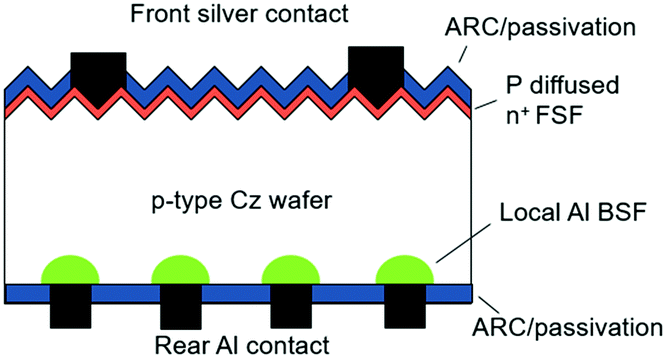
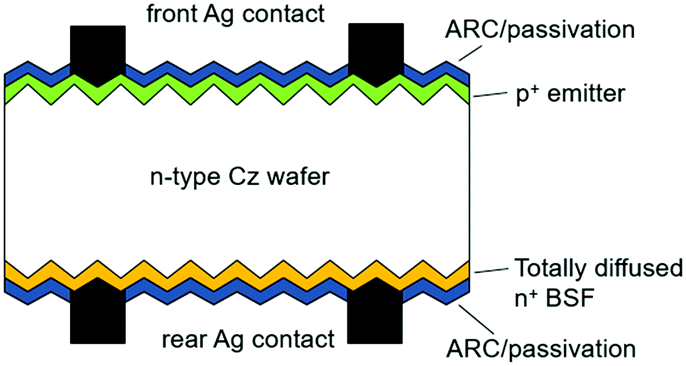
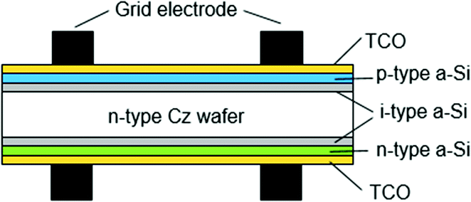
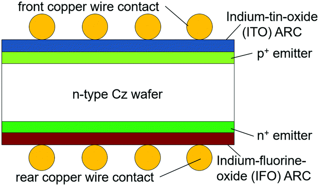
This section gives a brief overview of various c-Si bifacial PV cell and module technologies. As compared to the monofacial PV cells, bifacial PV cells offer other advantages besides being able to absorb irradiance from both sides. These advantages are (1) the reduction of electrical loss due to parasitic light absorption in the aluminium and high surface recombination at the metal–silicon interface of the Al back surface field (BSF);33–35 and (2) avoidance of the warping effect due to the difference in thermal expansion between aluminium and silicon.36 A summary of various c-Si bifacial PV cell technologies, including the cross-sectional schematics of each bifacial PV cell structure, is given in Table 2. The table also outlines the efficiency and bifaciality of some cell technologies.| c-Si cell technology | Description | Schematic of the cell structure |
|---|---|---|
| Bifacial PERC | • Acronym for passivated emitter rear contact |
|
| • Efficiency: 19.4–21.2% (front), 16.7–18.1% (rear)53,54 | ||
| • Bifaciality: ∼80%54 | ||
| • Mainly based on p-type crystalline silicon (c-Si) wafer | ||
| • The cell structure was used for studying the Shockley–Read–Hall recombination velocity at the Si–SiO2 interface55,56 during 1988 and 1991 | ||
| • It was introduced as a new bifacial PV cell in 199653 | ||
| • ISF Hamelin54 and SolarWorld57 demonstrated the industrial bifacial PERC (or PERC+) design for mass production | ||
| PERL | • Acronym for passivated emitter rear locally-diffused |

|
| • Efficiency: 19.8% (front)58 | ||
| • Bifaciality: ≥89%58 | ||
| • Mainly based on p-type c-Si wafer | ||
| • Boron is locally diffused into contact areas at the rear side59 | ||
| PERT | • Acronym for passivated emitter rear totally diffused |
|
| • Efficiency: 19.5–22% (front), 17–19% (rear)60–64 | ||
| • Bifaciality: ≥85%60,61 | ||
| • Commercialised based on the n-type c-Si wafer; also based on p-type65 | ||
| • PVGS developed n-type EarthOn™ cell in 200960 | ||
| • ECN developed n-Pasha (passivated all-sides H-pattern) cell to reduce yield loss; it was commercialised by Yingli Solar as PANDA61 | ||
| • N-MWT (Metal Wrap Through) was also proposed by ECN to narrow down busbars and reduce metal coverage66 | ||
| • ISC Konstanz developed BiSoN cell and commercialised by MegaCell67 | ||
| IBC | • Acronym for interdigitated back contact |

|
| • Efficiency: 23.2%68 | ||
| • Bifaciality: 75%69 | ||
| • Mainly based on n-type c-Si wafer | ||
| • No metal grid contact at the front side, first introduced by Bell Labs in 195470 | ||
| • ISC Konstanz perfected the production process and introduced ZEBRA cell71,72 | ||
| • ECN proposed Mercury cell with front floating emitter (FFE)73,74 | ||
| HIT | • Acronym for heterojunction with intrinsic thin-layer |
|
| • Efficiency: 24.7%75 | ||
| • Bifaciality: >95%76 | ||
| • Mainly based on n-type c-Si wafer | ||
| • Introduced by Sanyo (now Panasonic) in 1997 and entered into the serial production under the brand name HIT®75,77,78 | ||
| • Bifacial HIT® cell was introduced by Sanyo (now Panasonic) in 2000 and entered into the serial production76,79 | ||
| • Basic technology patent was discontinued and opened to the public in 2010; Meyer Burger adopted the cell technology80 | ||
| DSBCSC | • Acronym for double-sided buried contact solar cell |

|
| • Efficiency: 22%81,82 | ||
| • Bifaciality: 74%83 | ||
| • Plated metal contact is entrenched in the laser-formed grove | ||
| • Low resistance and low shading losses, due to high metal aspect ratios and lightly diffused emitter81 | ||
| Sliver® | • Developed at the Centre for Sustainable Energy Systems, Australian National University84 |

|
| • Efficiency: 19.4%84 | ||
| • Narrow groves are created via conventional micro-machining technique, forming a series of thin silicon strips85 | ||
| • Reduces silicon consumption by up to a factor of 1085 | ||
| BICONTY | • Acronym for bifacial concentrator n-type |
|
| • Efficiency: 17.6% (front), 16.7% (rear)86 | ||
| • Based on the laminated grid n-type solar cell86 | ||
| • Silver free – uses copper wire coated with low-temperature solder, resulting in very low shadow loss and resistance loss86 | ||
The potential of bifacial PV cells is fully realised when encapsulated in a glass/glass module structure to allow absorption of the ground-reflected and diffuse irradiance incident on the rear side of the glass/glass module, thus increasing the energy yield.37 Also, frameless glass/glass modules offer additional mechanical strength and provide resistance against moisture ingress, thermally induced degradation and potential induced degradation (PID).38–41 On the other hand, encapsulating bifacial PV cells in a glass/backsheet structure increases module current and power, the reasons being (1) the transmittance of longer wavelengths through the bifacial PV cell and subsequent backscattering at the backsheet; and (2) the scattering in the cell-gap region by backsheet and subsequent reflection at the air–glass interface.37 Nonetheless, the choice of module structure depends on the required applications.
Various technologies have also been developed to make the most out of the bifacial PV cell structures, which is by minimising the resistive and optical losses. The resistive loss is reduced through advanced interconnection technologies, such as Meyer Burger's Smart Wire Connection Technology (SWCT),42 SCHMID's Multi-busbar43 and APOLLON Solar's NICE (New Industrial Solar Cell Encapsulation) technology.44 In principle, using a small wire (busbar-less) or multiple busbars (more than three busbars) achieves lower series resistance due to the presence of a longer current path, shorter effective finger length (or smaller finger thickness) and more uniform current distribution.42,45 Other advantages of the small-size wire include the alleviation of cell breakage, mitigation of thermal stress on the wafer and reduction of silver paste consumption (and production cost). Furthermore, cutting the PV cells by half reduces the resistive power loss fourfold.46 Khoo et al.47 show that combining half-cut cells and multiple busbars could provide a 4% power gain, as compared to a three-busbar full-size cell.
Additionally, small wire and multi-busbar designs minimise the optical loss through reduction of the shading on the cell's active area and reduction of the light reflectance or absorbance by inactive area. Similarly, shingled interconnection minimises optical loss while increasing the module power density.48 Likewise, application of selective reflective coatings, e.g., infra-red (IR) reflective coating on the rear glass and reflective coating within the cell gaps, reduces transmittance loss.47 ECN's white bifacial PV module49 and SolarWorld's Sunmodule Bisun protect50 also propose a similar use of the reflective coating within cell gaps and module edges to enhance STC power measurement while preserving the module's energy yield. If both IR reflective (on the rear glass) and reflective coatings (within cell gaps) were applied, a 4% current gain could be obtained.51 Lastly, DSM's polymeric light trapping film (LTF)52 improves the optical performance by trapping the incident irradiance with the regular texturing of single apex corner cubes.
3. Indoor and outdoor performance characterisation of bifacial PV devices
Characterisation plays a crucial role in research for improving the performance of PV cells and modules. From a commercial point of view, characterisation determines the value or selling price of the product based on its performance (for example, max power rating and efficiency) and helps manufacturers from different regions of the world to market their products globally. Characterisation also benefits consumers, utility companies or power system designers to size the appropriate system components, estimate the annual energy yield and calculate the installed capacity for PV systems.Standards published by the International Electrotechnical Commission, e.g., the IEC 60904 series, IEC 60891 and IEC 61853, are available for characterisation of monofacial PV cells and modules. The IEC 60904 series consists of multiple parts that describe the requirements for indoor characterisation of PV cells and modules under STC, and for outdoor performance assessment. The procedures for measuring current–voltage (I–V) characteristics, equivalent cell temperature, spectral mismatch, spectral responsivity and verifying the linearity of PV devices are laid down in parts 1, 5, 7, 8, and 10, respectively.87–91 Requirements and calibration procedures for PV reference devices, as well as reference spectral irradiation, are given in parts 2, 3, and 4.92–94 The performance requirements of solar simulator classification are specified in part 9.95
IEC 61853 is another important series of norms, covering indoor and outdoor test methods for determining mainly the energy rating of PV modules. The series includes irradiance and temperature performance and power rating (part 196); spectral responsivity and angle of incidence (AOI) effects and the estimation of module operating temperature from irradiance (part 297); the calculation of module energy rating in kW h (part 397); and the definition of reference irradiance and climatic profiles (part 497). At the time of writing, parts 3 and 4 are still under preparation.
Despite the apparent sophistication and inclusiveness (Working Group 2, the task force editing IEC standards for PV non-concentrating modules, is by far the most active group not only of the Technical Commission 82 – “Solar photovoltaic energy systems”, but of the entire IEC), the IEC standards are still far from covering all characterisation aspects of all possible PV devices for terrestrial applications. The most relevant examples are c-Si bifacial PV cells and modules.
The performance characterisation of bifacial PV devices remains challenging for various reasons. Firstly, both the front and rear sides of bifacial PV cells and modules produce electric current simultaneously. Therefore, the performance characterisation of bifacial PV cells and modules needs to incorporate the nature of bifacial illumination,98i.e., the amount of total and spectral irradiance impinging on the module on both sides. Secondly, the STC does not include the irradiance conditions on the rear side, which is sensitive to the irradiance components (the direct component, and most importantly the diffuse component and reflected component from the background, known as the “albedo”) and installation conditions, e.g., orientation, tilt, height from the ground and shading due to the neighbouring modules and arrays.99,100
Thirdly, characterising the bifacial PV modules with a glass/glass structure under STC produces lower efficiency or power density (power output per unit area) due to the transmittance of the back sheet and light-absorbing environment.101 The potential of bifacial PV modules is underestimated because, in reality, bifacial PV modules generate higher annual energy output than monofacial PV modules.70,102 It has been shown in the study performed by Yusufoglu et al.103 that a significant energy gain of up to 25% can be achieved by using bifacial PV modules under optimal outdoor conditions.
In the absence of dedicated standards for bifacial PV cells and modules, industrial producers of bifacial modules often resolve to a variety of performance estimations and reporting methods. Most producers specify the front side electrical parameters (maximum power, short-circuit current, open-circuit voltage and efficiency) under STC and under different levels of additional rear-side irradiance, in which some are termed “bifacial gain” or “backside power boost”.104–107 The details of quantification – whether the electrical parameters corresponding to each level of additional rear-side irradiance are measured or extrapolated – are not specified. Some producers adopt “equivalent efficiency”, which is the “efficiency of the monofacial PV cell needed for generating the same energy as a bifacial PV cell under the given conditions”.108 For some electrical specifications, the efficiency and maximum power appear to be exhibiting a linear relationship with rear-side irradiance. However, it was pointed out that such results are inaccurate because the electrical parameters of bifacial PV devices are naturally non-linear in response to the irradiance.109 Other producers such as Prism Solar adopt the “Bifacial STC” (BSTC), in which the bifacial PV modules are rated based on the front-side STC (1000 W m−2) and an additional 300 W m−2 of rear-side irradiance. According to Prism Solar, the short-circuit current, maximum power and efficiency can be estimated to be 127% of the front side (STC) values.110,111
3.1. Indoor performance characterisation of bifacial PV cells
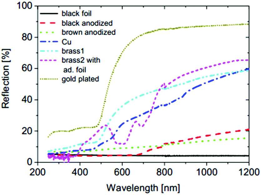
Generally, electrical parameters of the front and rear sides of the bifacial PV cells are characterised following the standard method for mono-facial cells (IEC 60904-1) and reported separately.54,60,112,113 The bifacial PV cell is secured to the metal chuck and exposed to the illumination of the solar simulator, which is located on top of the PV cell. The metal chuck provides electrical and thermal contacts between the PV cell and measurement device. However, it has been shown that a conventional measurement setup introduces inaccuracy for two reasons:114 reflectance and electrical conductance of the metal chuck. Long wavelength radiation (ranging between 900 and 1200 nm) transmits through the bifacial PV cells (as shown in Fig. 1) and reflects into the cell from the chuck surface.115 | ||
| Fig. 1 Reflectance of chucks made of different metals; gold chuck has the highest reflectance of more than 80%. Reprint from ref. 115. Permission granted by WIP. | ||
In the case of a gold-plated chuck with more than 80% of reflectance, as shown in Fig. 2, the short-circuit current is overestimated by about 1%.115 A similar trend was also reported by Duran et al.,116,117 in which a white chuck surface or surface with 85% of reflectance contributes to an overestimation of current density by 1%. According to Singh et al.,118 an overestimation of bifacial PV cells’ power and efficiency by more than 2% (relative) was reported when a conductive and reflective chuck was used. A conductive chuck provides more pathways for the generated current to flow through, resulting in lower series resistance between the chuck and rear metal contacts. In contrast, a non-conductive chuck only allows current to flow through the metal fingers at the rear side to busbars.118 A chuck with a non-reflective surface, for instance, black foil,115 presents a viable solution. However, the non-reflective surface usually has poor thermal conductance, which could result in cell heating and underestimation of open-circuit voltage.114
 | ||
| Fig. 2 Transmission of 4 different PV cells: (B) represents the fully bifacial cell; (A, C and D) represent back contact cells (bifaciality is the by-product of the cell technology). Reprint from ref. 115. Permission granted by WIP. | ||
Two parameters were proposed by Singh et al.119 to evaluate the bifacial characteristics of bifacial PV cells, namely the bifacial 1·x efficiency, η1·x (effective efficiency), and the gain-efficiency product (GEP). Both parameters are calculated using separate measurements of front-side and rear-side electrical parameters. The bifacial 1·x efficiency is defined as
 | (1) |
 is the current increment due to bifacial illumination compared to monofacial illumination; g is a factor referred to as the “irradiance gain”; Voc-bi and Voc-f are the open-circuit voltage of the bifacial device and only the front side, respectively. FFbi and FFf are the fill factor of the bifacial device and only the front side, respectively.
Derivation of η1·x is based on the assumption of linearity of the bifacial cell short-circuit current, Iscversus the irradiance, or equivalently, the total photo-generated current of the bifacial PV cell is given by the sum of the currents generated from the front and rear sides. The factor  can thus be shown to be:
 | (2) |
The irradiance gain due to the additional illumination at the rear side is thus
 | (3) |
The expressions of Voc-bi and FFbi are given as
 | (4) |
 | (5) |
 | (6) |
The second parameter, gain-efficiency product (GEP), is the combination of g and η1·x. As shown in Fig. 3, at higher irradiance gain, cell-A has higher η1·x (higher performance) than cell-B, although cell-B has higher front-side efficiency than cell-A (front-side efficiency of cell-A and cell-B are 16.85% and 17.32%, respectively). Irradiance gain refers to the additional rear-side irradiance, i.e., g = 1.6 corresponds to 600 W m−2 total irradiance from the rear side, when the front side is at 1000 W m−2, the standard irradiance (given that x = 60%). The result of Fig. 3 implies that front- and rear-side efficiency alone does not reflect the actual performance of bifacial PV cells. In other words, actual performance relies on the simultaneous (bifacial) illumination and non-linear combined characteristic of the front and rear sides.
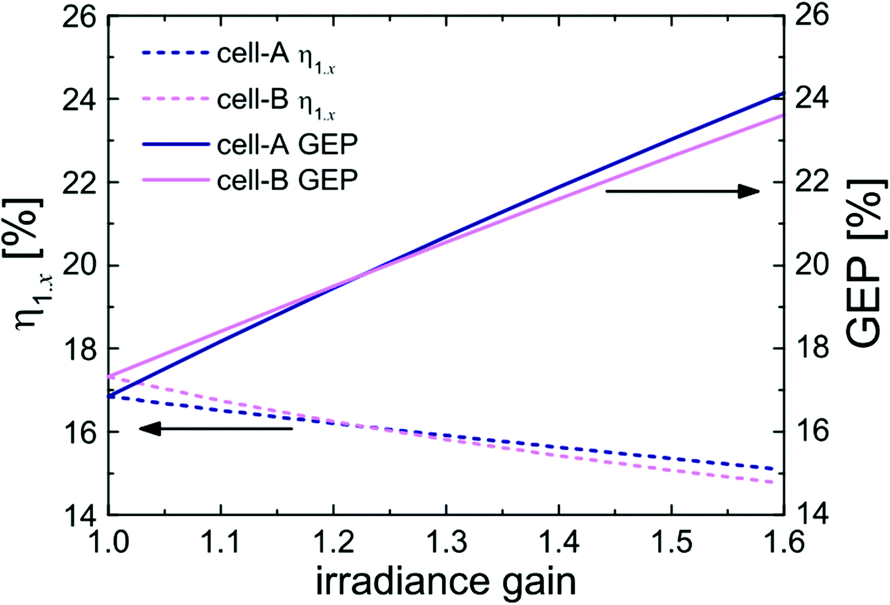 | ||
| Fig. 3 The relationship of η1·x and gain-efficiency product (GEP) with respect to the irradiance gain g. Reprint from ref. 119. Copyright 2012, John Wiley & Sons, Ltd. | ||
A bifacial illumination (simultaneous illumination) setup was used by research groups from Japan and Europe for characterising the bifacial PV cells. Assembled by CENER (National Renewable Energy Center of Spain), the Bifacial Cell Tester (BCT)120 consists of a vertical cell holder standing equidistantly between two mirrors that are tilted 45° from the cell holder. The schematic diagram and side-view of the BCT are shown in Fig. 4. The bifacial test cell and the reference cell are secured vertically by the cell holder. The tester can accommodate PV cells with size up to 156 × 156 mm2. I–V measurements are recorded using four current contact probes (two for each side and a total of 16 current collecting points) and one voltage probe per side. A 10 ms pulse class-A flash simulator is located perpendicular to the base. Pulse illumination ensures the constancy of cell temperature during measurements. Following the IEC 60904-9, a value of lower than 2% is achieved for spatial uniformity and temporal stability. Additionally, the BCT is put inside the temperature-controlled area to maintain the bifacial test cell's temperature at 25 ± 2 °C. The glass mirrors reflect the illumination from the light source to the reference cell and bifacial test cell. One mirror simulates the lighting onto the front side of the cell. The other mirror, coupled with filter meshes, simulates the lighting of reduced intensity onto the rear side of the cell or albedo. The metal structure was painted black matte to minimise reflectance, while the glass mirror has over 80% of reflectance for wavelengths ranging from 400 nm to 1100 nm.
 | ||
| Fig. 4 Schematic diagram of a bifacial cell tester. Reprint from ref. 120. Permission granted by WIP. | ||
The measurement setup used by the Central Research Laboratory, Hitachi Ltd, in Japan121 to investigate the characteristics of bifacial PV cells with various rear structures resembles the BTC. Since the experimental procedures do not include the variation of irradiance levels between front and rear sides, filter mesh is not observed in the setup. Two parameters, namely, the bifacial illumination effect, Δ, and separation rate were given as:
| Δ = PM(n,n) − [PM(n,0) + PM(0,n)] | (7) |
 | (8) |
These two parameters were adopted by researchers at CENER as well. Given that the separation rate is about 1.0% and Δ is close to zero, both groups concluded that the current density under bifacial illumination at one Sun (n = 1), Jsc(1,1), is merely equal to the sum of Jsc(1,0) + Jsc(0,1). The conclusion coincides with the claim made by Singh et al.119
Using the BCT, M. Ezquer et al. shows that the fill factor (FF) of the I–V curve, which is characterised under bifacial illumination (one Sun on each side of the bifacial PV cell), is lower than the FF of the I–V curve that is obtained by summing the current values from each side under monofacial illumination.120 The results are shown in Fig. 5. These results, according to the reference, point out the incurring inaccuracy should the monofacial characterisation of bifacial PV cells be used to extrapolate the results to define the bifaciality characteristic.
 | ||
| Fig. 5 The cell current measured under bifacial illumination (represented by dark blue I–V curve) is lower than the sum of cell current for both sides under monofacial illumination (represented by magenta I–V curve). The yellow I–V curve represents the front-side cell current under monofacial illumination; the cyan I–V curve represents the rear-side cell current under monofacial illumination (P and N denote front and rear sides, respectively). Reprint from ref. 120. Permission granted by WIP. | ||
Although the BTC setup exhibits superiority over the conventional method with a chuck, it has yet to be compared with the simultaneous illumination setup (with the bifacial cell fixed on the vertical structure) using two solar simulators. The filter mesh in the equipment used at CENER does not allow precise manoeuvrability of rear-side illumination conditions (or albedo). Instead, a setup with two solar simulators can achieve that. Lastly, the fixture could include more current and voltage collector probes to accommodate new cell technologies, e.g., five busbars and multi-wire bifacial PV cells. Nonetheless, the design and position of probes have to be perfected to avoid non-uniformity of illumination due to the shading of bifacial PV cells.
Other measurement artefacts and resulting challenges in removing them may come from the measurement of the cell temperature (taken from the rear side of the PV device), the total irradiance of both sides (and therefore find the most appropriate positioning of the reference cells), and the spatial uniformity of the rear side irradiance (and spectral irradiance).
At the commercial level, h.a.l.m elektronik proposed two-light-source characterisation equipment for bifacial PV cells.122,123 The characterisation equipment uses two synchronised (but independently regulated) class AAA xenon light sources (as illustrated in Fig. 6). One light source is located on top of the measuring plane. The other light source is situated horizontally, at the bottom of the measuring plane. The titled mirror reflects the illumination from the bottom light source onto the rear side of the bifacial PV cell. The equipment is programmed to operate in various modes of the flash sequence. For instance, in a 90 ms flashing sequence, the bottom light source flashes at the STC irradiance level for the first 30 ms, followed by 30 ms of lower irradiance level (e.g., 200 W m−2); the top light source flashes at the STC irradiance level during the last 55 ms. In this flash sequence, the front side, rear side, and bifacial characterisation could be performed.
 | ||
| Fig. 6 The schematic of h.a.l.m elektronik's xenon flasher: cetisPV-IUCT-BF (left); one example of flashing sequence (right). Reprint from ref. 123. Permission granted by h.a.l.m elektronik. | ||
3.2. Indoor performance characterisation of bifacial PV modules
 | (9) |
The term represents the ratio of the short-circuit currents for the front and rear sides of bifacial PV modules. Then BiFiIsc is applied in the following equation to calculate the bifacial equivalent irradiance, GE:
| GE = 1000 W m−2 + BiFiIsc·Grear | (10) |
G. Razongles et al.99 derived equations to extrapolate the maximum power rating of bifacial PV modules corresponding to different front- and rear-side illumination. The main equation is given as
| Pmax(S) = S·f·Pmax | (11) |
 | (12) |
f = 1 + a·(S − 1) + b·ln![[thin space (1/6-em)]](https://www.rsc.org/images/entities/char_2009.gif) S + c·(S − 1)2 + d·(lnS)2 S + c·(S − 1)2 + d·(lnS)2 | (13) |
Eqn (12) and (13) were taken from the MotherPV method.127 The number of Suns, S, refers to the ratio between front-side irradiance and the STC value (1000 W m−2). Eqn (13) is the polynomial function of the neperian logarithm;127a, b, c, and d are constants. The parameter f represents the “irradiance coefficient”. The maximum power, Pmax, was measured by flashing the front side at an equivalent irradiance, given as
 | (14) |
Alternatively, Corbellini and Medici128 calculated the bifaciality factor using the STC power of the front and rear sides, which is expressed as
 | (15) |
Accordingly, the unintended irradiance on the non-illuminated side was quantified and included in the single-sided STC power measurements. It was measured repeatedly using a reference cell at several positions on the non-illuminated side. The ratio of the irradiance on these positions concerning the irradiance on the illuminated side (also measured using a reference cell) was calculated. The lowest ratio was taken to correct the STC power measurements for both front and rear sides.
A set of equations based on the one-diode equivalent model was proposed by Singh et al.109 to calculate the power and efficiency of bifacial PV modules. This method is different from the equivalent irradiance method, whereby the bifacial electrical parameters can be calculated directly from the STC measurements of the front and rear sides without going through the second front-side flashing with equivalent irradiance, GE. The equations are given as
| Pbi = Isc-bi·Voc-bi·FFbi | (16) |
 | (17) |
 | (18) |
 | (19) |
 | (20) |
 is described in the previous section, while pFF is now given by
 | (21) |
Several assumptions were made for this method. Firstly, the Isc of the bifacial PV module under bifacial illumination is the sum of short-circuit currents for the front and rear sides under monofacial illumination. Secondly, no stray light enters the module when the short-circuit currents of the front and rear sides are measured separately under STC. A black cloth is used to cover the non-illuminated side. Thirdly, the operating current changes corresponding to the irradiance, similar to the short-circuit current. Lastly, pFF does not change with the irradiance.
The deviations of Isc, Voc, η, and FF between measurement and numerical simulation are within 1%, which indicate the negligible effects the assumptions have on the accuracy of results. Nonetheless, lower simulated FF value at higher irradiance suggests that this method is more appropriate for PV modules with a high fill-factor (preferably more than 75%) because for low FF PV modules under high irradiance, the third assumption slightly overestimates the module operating current and resistive losses. Alternatively, Deline et al.124 formulated an equation to obtain pFF, which is used for calculating FFbi with eqn (20). The equation is given as
 | (22) |
The series resistance, Rs, is approximated by the slope on an I–V curve of a PV module at Voc-f.
A setup (shown in Fig. 7), similar to the BCT, was used by Razongles et al.99 and Soria et al.130 to conduct bifacial PV mini-module (of four cells) characterisation. The angle between the mirrors and bifacial PV module was optimised (44.1° instead of 45°) to reduce the influence of angle.130 To date, no attempt has been made to scale up the setup for full-size bifacial PV module characterisation.
 | ||
| Fig. 7 Two-mirror setup for bifacial PV module characterisation. Reprint from ref. 99. Licensed under CC BY-NC-ND. | ||
 | ||
| Fig. 8 A bifacial illumination setup using two identical solar simulators, proposed by Eternal Sun. Reprint from ref. 99. Licensed under CC BY-NC-ND. | ||
 | ||
| Fig. 9 A bifacial illumination setup proposed by h.a.l.m. Reprint from ref. 129. Permission granted by h.a.l.m elektronik. | ||
Theoretically, two simulators should be controlled concurrently by a single control system to avoid systematic error due to lagging or mismatch between the flashing sequence of both simulators. It is also possible that illumination on one side of the bifacial PV module will interfere (constructively or destructively) with the illumination on the other side of the module through transmittance and reflection of irradiance between and through cells, thereby introducing irradiance non-uniformity and inconsistencies. The Swiss company Pasan SA, which is the subsidiary of Meyer-Burger Technology AG, also proposes a commercial double-light source solution, via merely doubling its existing multi-lamp Xenon module simulator. In this case, the distance between the two light sources (approximately 16 metres) may help reduce the interferences between the two light sources, but the space needed to host such equipment and its cost may be challenging for the customer.
On the other hand, replacing the conventional light source, such as the xenon lamp, with LED light enables variation of spectral irradiances (spectral distributions).131,132 It could enhance the prediction of real-world performance or simulate the rear-side irradiance conditions that are probably closer to the diffuse component of AM1.5G than AM1.5G itself (the standard reference irradiance for both front and rear sides of the module, according to the draft version of IEC TS 60904-1-2, as discussed in Section 3.5 below). The LED-based solar simulator achieving Class AAA has been made commercially available133 but is yet to be adapted for simultaneous illumination (double-light sources). In conclusion, the spatial requirement and the cost of deploying two solar simulators remain to be the fundamental challenges. It would, therefore, be useful to conduct a cost–benefit analysis to justify the accuracy of measurement results for the required setup cost.
3.3. Outdoor performance characterisation of bifacial PV modules
Outdoor measurements are beneficial and necessary because the practices allow the measurement of PV modules under real operating conditions and are ideally free from the spectral mismatch. Nonetheless, in reality, they are more challenging for several reasons which make indoor measurements more accepted. Among these reasons, the most challenging one is to keep the module at the standard 25 °C cell temperature when the irradiance is at the standard 1000 W m−2. Apart from that, the need for stable and clear sky conditions is rarely achieved in many locations due to the weather variability.Generally, outdoor measurements of bifacial PV modules have two main purposes:
• Investigating and improving the performance of bifacial PV modules in real installations;
• Characterising the performance of bifacial PV modules (power rating) under actual environmental conditions.
There is a clear distinction between the methodologies of these two purposes. The first purpose involves a variation of multiple parameters (installation and geographical), e.g., height of the module from the ground, ground reflectance (albedo), tilt, azimuth angle, and location, to evaluate and validate the influence of each parameter on the bifacial performance.102,126,134,135 Moreover, the simulation results could be compared to the outdoor measurements to verify the accuracy of the simulation model. Details of the bifacial PV performance modelling are elaborated in Section 3. The second purpose measures the bifacial performance under fixed installation and geographical conditions,2,124,136 to match as close as possible the STC without the need for expensive equipment for the (mono or double) light source. This section primarily discusses the second purpose – outdoor characterisation of bifacial PV modules.
The I–V characteristic and maximum power can be recorded via commercially available measurement devices, such as PVPM 2540C (PVE Photovoltaik Engineering, Germany) and MP170 (EKO, Japan).136 A pyranometer and reference cells are used for measuring irradiance components (global, direct or diffuse) impinging the front side of bifacial PV modules. The albedo can be measured using an albedometer (e.g., Schenk's Dualpyranometer,137 CMA11, Kipp and Zonen,138 and SRA01, Hukseflux139), which is mainly composed of two identical pyranometers offsetting at 180° – one facing upward to measure the global irradiance and the other facing downward to measure the reflected irradiance. As pointed out by Pirazzini,140 the albedometer has to maintain horizontal alignment and a certain height from the ground to reduce the measurement errors. Another important consideration is the deviation from the ideal cosine response; the author mentioned that error increases as the zenith angle increases from 80° for albedo measurement over high latitude sites.
More than a decade ago, D. Faiman et al.141 proposed an outdoor method to assess the front- and rear-side efficiencies. Two identical bifacial PV modules are positioned horizontally above ground to ensure an unobstructed view of the ground. One module has its front side facing upwards and the other being inverted (front side facing downwards). The power values generated by upward-facing and downward-facing modules (Pu and Pd, respectively) are calculated as
| Pu = G·A·(ηf − α·ηr) | (23) |
| Pd = G·A·(ηr − α·ηf) | (24) |
 | (25) |
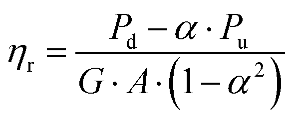 | (26) |
Albedo is measured by a pair of monofacial PV modules (one facing upwards and the other facing downwards) with close spectral sensitivity to the bifacial PV module. The effective efficiency compares the electrical output and incident insolation on the front side of the bifacial PV module. The results show that the monofacial PV module efficiency is higher than the effective efficiency of the bifacial PV module. Lastly, the efficiency varies according to the module orientation.
A comprehensive description of outdoor characterisation was presented by Deline et al.124 Because the objective was to verify the results of indoor characterisation, the outdoor measurement conditions were adjusted carefully to the indoor conditions. The bifacial PV module under testing was secured on an open-frame rack. The tilt angle and orientation of the rack were changed to achieve close to 1000 W m−2 of front irradiance. Front irradiance was measured by a reference cell. Rear-side irradiance uniformity was measured by fixing three reference cells at different locations of the rear side. The spectral response and incident-angle of reference cells were matched closely to the module. Non-uniformity, expressed as below, is less than 5%:
 | (27) |
Low rear irradiance non-uniformity requires refinement of near ground cover. This procedure eliminates the inhomogeneity of rear-side irradiance, an outdoor anomaly mentioned in the study conducted by Razongles et al.99 A module temperature of 25 °C is achievable during winter; for warmer ambient, e.g., during other seasons and in the tropic region, temperature correction is required. The influence of cell gaps (transmittance of irradiance through the cell gaps) on rear-side irradiance was minimised with sufficient module height from the ground. Different levels of rear irradiance, Gr, were obtained by altering the albedo, e.g., covering the ground with a reflective white sheet for high Gr and black opaque sheet for low Gr. The comparison between indoor (single-sided illumination) and outdoor measurements concludes that the results of indoor and outdoor characterisations for various types of bifacial PV modules agree within 2%. Results are shown in Fig. 10.
 | ||
| Fig. 10 Outdoor and indoor characterisations of module A (left) and module B (right) agree within 2%. Reprint from ref. 124. Copyright 2017, IEEE. | ||
Both studies reflect the differences between the dominance of indoor or outdoor characterisation over the other and the associated requirements. When the indoor measurement serves to verify the outdoor characterisation, the indoor measurement method has to be designed and improved in such a way that it could accurately simulate the real world conditions. Vice versa, outdoor measurements have to be adjusted to produce matching results. Given that the actual world performance differs geographically (regionally), in which the altitude, topography, weather or sky conditions play a deterministic role, the long-term research focus should be on using outdoor measurements to define parameters that affect the real world performance and incorporating these parameters into indoor measurement. Alternatively, the report of performance rating for bifacial PV modules could include both indoor and outdoor measurement results, whereby the geographical and installation conditions are highlighted. This is similar to the climatic profiles that are introduced in IEC 61853 Part 4, for correcting the monofacial PV modules’ power and energy rating.96
3.4. The technical specification – IEC TS 60904-1-2
A draft technical specification, designated as IEC TS 60904-1-2, has been proposed for standardising the indoor and outdoor characterisation of bifacial PV cells and modules.142–144 The document has been submitted to IEC for publication, at the time of writing, and is expected to be published at the beginning of 2019. The procedures specified in this draft standard are based on the same principles as in the IEC 60904-1, with additional requirements dedicated to the bifacial PV devices.The draft technical specification classifies indoor characterisation to single-sided and double-sided illuminations. For indoor characterisation using single-sided illumination, the solar simulator must provide more than 1000 W m−2 of irradiance level at less than 5% of non-uniformity. Two conditions are specified to reduce the irradiance on the non-illuminated side, which is limited to 3 W m−2. Firstly, the non-reflective material is located at a certain distance from the non-illuminated side. Secondly, the bifacial PV device under testing is fixed to an aperture to limit the exposure of the test area to illumination within the size of the test device. For evaluation of the irradiance and uniformity on the non-illuminated side, the draft requires at least five measurements at the symmetrical points (as shown in Fig. 11, right), for instance, P1–P3–P5–P7–P9.
 | ||
| Fig. 11 Left: Positions of reference devices for outdoor measurement. Right: Positions for measuring the non-uniformity of rear-side irradiance (at least 5 symmetrical positions). | ||
The draft also specifies calculation of bifaciality coefficients and power generation gain for single-sided illumination. Bifacial coefficients correlate the characteristics of the front and rear sides, which are measured separately under STC:
 | (28) |
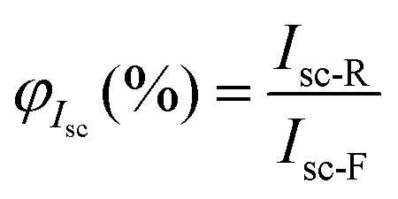 | (29) |
 | (30) |
| GEi = 1000 W m−2 + φ·GRi | (31) |
| φ = Min(φIsc,φPmax) | (32) |
The double-sided illumination refers to the use of a solar simulator that is capable of illuminating both sides of bifacial PV devices simultaneously. Similarly, for indoor characterisation using double-sided illumination, the non-uniformity should be less than 5% of the irradiance level on both sides. Besides that, the procedures should take into account the geometry of the bifacial PV modules on assessing the non-uniformity of illumination.
For outdoor characterisation, besides the PV reference device facing the sun, at least two PV reference devices are required to measure the rear-side irradiance and non-uniformity (as shown in Fig. 11, left). The non-uniformity of rear-side irradiance should not be more than 10%. In order to measure the non-uniformity of rear-side irradiance for the outdoor measurement, at least five symmetrical points on the rear side of the bifacial PV module, for instance, P1–P3–P5–P7–P9 (as shown in Fig. 11, right) are selected.142 The uniformity of reflected light in outdoor measurements can be increased by using a reflective cloth and raising the bifacial PV devices. However, the cloth reflectivity and height of the bifacial PV devices from the ground are not specified.
The power generation gain for indoor measurement with double-sided illumination and outdoor characterisations are measured at
| 1000 W m−2 on the front side + GRi | (33) |
3.5. Reference spectral irradiance: spectral mismatch correction and effect of the albedo
The reference standard spectral irradiance for both the front- and rear-side illumination, according to the IEC TS 60904-1-2, is AM1.5G (for indoor characterisation using single-sided and double-sided illuminations, as well as outdoor characterisation). AM1.5G is the standard “global” spectrum defined in IEC 60904-3 – a combination of the “direct” spectrum (also defined in IEC 60904-3 as AM1.5D, the flux of light coming straight from the Sun in direct normal incidence) and the “diffuse” spectrum from the sky (defined as the subtraction of AM1.5D from AM1.5G).It may seem poorly logical to rate the power of a bifacial PV module with rear-side illumination corrected to the “global” spectrum, as under real operating conditions the rear side “sees” the albedo, which is often almost entirely diffuse spectrum with little direct component. This argument is always true when the bifacial PV module is on the tracker and has the most limited validity on vertical installation with east–west orientation (where reasonably the two sides of a bifacial PV module respond symmetrically to the incoming global irradiance during the day).
At least two alternative approaches to the one currently described in IEC TS 60904-1-2 may have been chosen:
(1) To use AM1.5G for the front side, and the “diffuse” spectral irradiance for the rear side. Both spectra are standardised in IEC 60904-3. Therefore, this choice would have no problem under the normative evaluation. However, there are at least two shortcomings. Firstly, two different spectral mismatch corrections for the front and rear sides would be needed, which could be quickly done for the double-sided illumination and outdoor characterisations; but would be less straightforward in the one-source method, requiring careful calculation of the equivalent irradiance, GE. Secondly, the albedo is not equivalent to the diffuse spectrum, and in specific applications it may in principle be as different from the diffuse component of AM1.5G as it is different from the AM1.5G itself, thus limiting the strength of the rationale of this approach.
(2) To define a “standard albedo” in addition to the spectra defined in IEC 60904-3 and to correct the rear side measurement for a spectral mismatch to this newly defined spectral irradiance.
These two approaches generally have an increased degree of complexity, both metrologically and administratively, as introducing a new standard spectrum is a significant change with respect to using the existing one. Furthermore, IEC TS 60904-1-2 is intended to be a labelling standard, not an energy yield calculation. Therefore, both the front and rear side reference spectra are specified as AM1.5G as a deliberate choice, given the scope of this document.
In the near future, the IEC 61853 will need to tackle the problem for bifacial PV modules deployed under real operating conditions, in which the spectral content of the rear-side illumination entirely depends on the variability of the albedo. At the time of writing, the WG2 of IEC/TC82 has not yet started a project team on amendment or revision of IEC 61853 or of parts of it, but such a project is expected in the years to come. The only possible approach currently applicable is to monitor the spectral variability of the albedo in the particular installation under study and perform spectral mismatch correction to the reference standard AM1.5G, according to IEC 61853-3.
4. Bifacial PV performance modelling
Various models are available to predict the real-world performance of bifacial PV modules and arrays (system). A typical simulation of real-world bifacial module performance, as shown in Fig. 12, consists of three models, namely optical (irradiance), electrical, and thermal models. Solar and meteorological data, including global horizontal irradiance (GHI), diffuse horizontal irradiance (DHI), ambient temperature (Tambient), and wind speed (νwind) are required as the input for the model.145,146 Solar data can be measured by a satellite, ground measuring station or a combination of both. It can also be downloaded from the database provided by companies such as Meteonorm147 or Solargis148 or, with some limitations, from free databases such as the Photovoltaic Geographical Information System (PVGIS,149).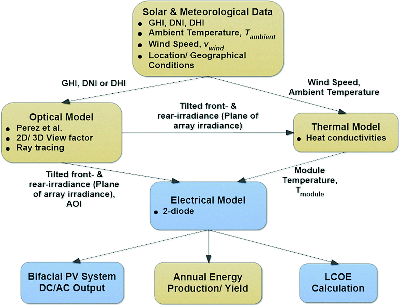 | ||
| Fig. 12 Schematic of a typical framework for simulating the real-world performance of bifacial PV modules or arrays (system). | ||
Optical and thermal models transform the meteorological data into the input data for the electrical model (front irradiance and rear irradiance, angle of incidence (AOI), and module temperature, Tmodule). The thermal model also relies on the optical model for front- and rear-side irradiances, which are combined with ambient temperatures and wind speeds to simulate the module temperatures. The output, which is generated from the electrical model, can be the DC (direct current) or AC (alternating current) power, or the annual energy production/yield of the bifacial PV modules or arrays (system). Annual energy production data, coupled with available cost and financial data (e.g., project cost, operational and maintenance costs, tax rate, and discount rate) could be used to calculate the LCOE of the bifacial PV systems. One of the main differences between the performance simulation of monofacial and bifacial modules is in the optical model. Hence, this paper focuses more on the review of the optical models.
4.1. Optical model
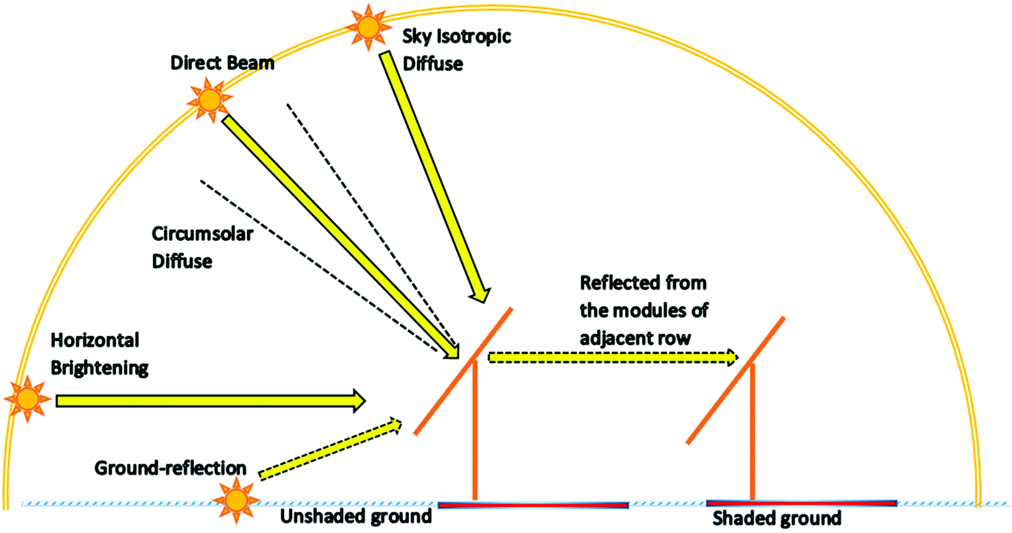 | ||
| Fig. 13 Schematic showing the irradiance components for the front-side irradiance. | ||
In the real world, PV modules are positioned at a specific orientation and tilt angle to harness the maximum solar energy. Using the measured GHI and DHI, the optical model for monofacial PV modules translates the incident irradiance on a horizontal surface to that of a tilted surface. The same concept can be used to calculate the total irradiance on the front side of a tilted bifacial PV module, which is expressed as
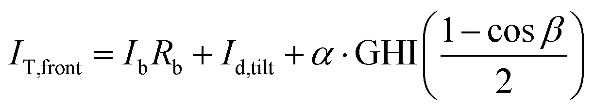 | (34) |
The three terms on the right of eqn (34) represent all the components of irradiance to the front side of the bifacial module, which are defined as follows:
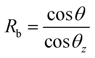
• IbRb is the direct irradiance component, where Ib is the direct normal irradiance (DNI) or beam irradiance of a horizontal surface. Rb is the ratio of the beam radiation on a tilted surface to that on a horizontal surface at any time, given by
 | (35) |
• Id,tilt is the diffuse component due to tilted irradiance. It can be estimated using three transposition models proposed by Liu and Jordan, Klucher and Perez et al.150 The Perez et al. model is preferred over Liu and Jordan as well as Klucher models because it considers all three components of diffuse irradiance (sky isotropic diffuse, circumsolar diffuse and horizontal brightening).150 The model calculates these diffuse components using empirical coefficients that are obtained based on various sky conditions. A complete account of the Perez et al. model can be read from the respective literature.151–153 Based on the Perez et al. model, the total tilted diffuse irradiance is
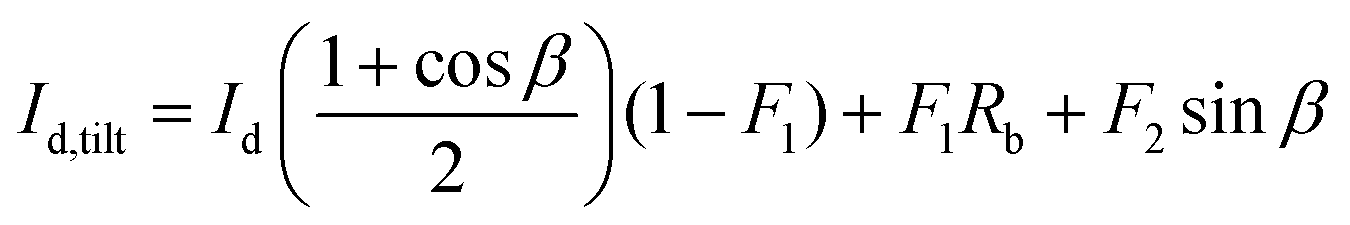 | (36) |
| F1 = f11(ε) + Δf12(ε) + θzf13(ε) | (37) |
| F2 = f21(ε) + Δf22(ε) + θzf23(ε), | (38) |
• The last term is the diffuse component contributed by the ground reflection. It is determined using the isotropic model proposed by Ineichen et al.154,155α is the albedo (or ground reflectance), which is assumed to be uniform across the underlying ground surface.156 [(1 − cosβ)/2] is the view factor between the front side of the bifacial PV module and the ground, assuming: (1) infinitely long rows; (2) no shading on the ground; (3) horizontal ground; and (4) ground is a Lambertian reflector, i.e., an isotropic scattering of irradiance by the surface irrespective of the nature of the incident irradiance.157,158 The concept of view factor is discussed in the next section.
Lastly, angular reflection losses and spectral mismatch are taken into account. Martin and Ruiz's IAM model159 provides an accurate prediction of angular reflection losses as compared to ASHRAE and physical IAM models, whereas Khoo et al.160 proposed a model to calculate the angular reflection losses of a module with textured front glass. On the other hand, King et al.'s model161 or mismatch factor89 can be adopted for spectral mismatch correction.
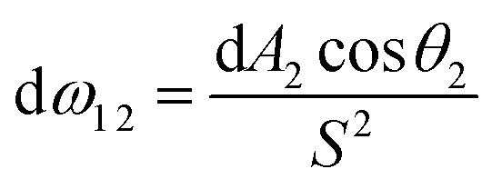
4.1.2.1. View factor model. Modelling the direct and diffuse components of rear side irradiance follows a similar fashion to that for the front side, with extra attention being given to θ, θz, and β. However, the main irradiance source – the ground-reflected irradiance – requires a more comprehensive analysis. Originated from the heat transfer or radiative transfer fundamentals, the concept of view factor (also known as shape factor, configuration factor or angle factor162) is adopted to model the irradiance reflected by ground and received by the rear side of bifacial PV modules.103,158,163,164 This concept is explained as follows.
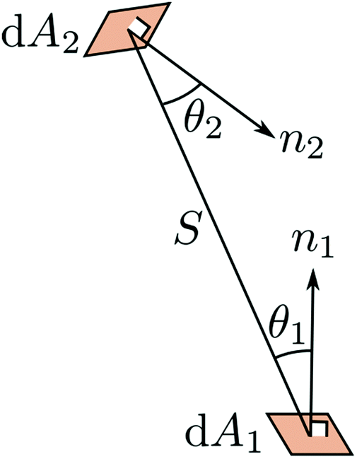
A geometrical relationship between two infinitesimal surfaces dA1 and dA2 is illustrated in Fig. 14. The differential surface dA2 is the irradiated surface (the rear side of the bifacial module) that receives a fraction of diffusely distributed radiation emanating from the differential surface dA1 (the ground reflecting surface). The surfaces are assumed to be the Lambertian reflector. The ratio between the energy irradiating dA2 over the energy irradiating from dA1, FdA1→dA2 is given by:155
 | (39) |
 | (40) |
 | (41) |
| A1FA1→A2 = A2FA2→A1 | (42) |
 | ||
| Fig. 14 Geometrical relationship between radiating and irradiated surfaces. | ||
The expression is known as the reciprocity rule. Finally, FA1→A2 is calculated as the integral of fractions of radiation leaving dA1 and reaching dA2. It is expressed as103
 | (43) |
Visual representation of the abovementioned formula is shown in Fig. 15. The formula is used for calculating the view factor between the module and ground. The subscripts “s” and “ns” indicate shaded and unshaded grounds respectively. As a result, the ground-reflected irradiance is given as:
| Irear,reflected = α·GHI·FRns→module + α·DHI·FRs→module | (44) |
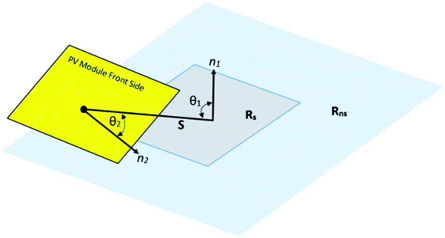 | ||
| Fig. 15 Corresponding denotations for the formula of view factor. | ||
• The first term on the right side of the formula represents the reflected irradiance from the unshaded ground, Rns, to the rear side of the bifacial PV module at the given ground albedo α. The unshaded ground reflects both DNI (direct normal irradiance) and DHI.
• The second term represents the reflected irradiance from the shaded ground, Rs, at the given albedo. DNI casts a shadow on the ground when the module blocks it. Therefore, the shaded ground only reflects the DHI.
To solve eqn (43) and (44), Shoukry et al.165 adopt the concept proposed by Gross et al.,166 in which the expression of view factor for two rectangular surfaces of a different plane, having parallel boundaries, is given as:
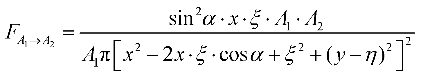 | (45) |
Referring to Fig. 16 (top), α is the inclination angle between two parallel planes (each plane carries one surface); x and y are the Cartesian coordinates of one plane (carrying surface A1), while ξ and η are the Cartesian coordinates of the other plane (carrying surface A2). An underlying assumption for eqn (45) is that the distance between A1 and A2 is large as compared to the size of A1 and A2, therefore the changes in direction angles from point to point of the areas are insignificant. As a result, x, y, ξ, and η are assumed as the centre coordinates of A1 and A2. Using eqn (45) to calculate directly the view factor of the module or array might be invalid, since it contradicts the underlying assumption when the surfaces of A1 and A2 are larger than the distance between two surfaces.
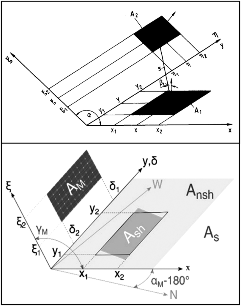 | ||
| Fig. 16 (top) Illustration of view factor calculation proposed by Gross et al. Reprint from ref. 166. Copyright 1981, Elsevier. (bottom) Gross et al. model was modified by Shoukry et al. to consider unshaded and shaded grounds. Reprint from ref. 165. Licensed under CC BY-NC-ND. | ||
The module shadow (Ash) is superimposed on the total underlying ground surface (AS) to determine the view factor between the shaded ground and rear side of the module, FAsh→AM (as shown in Fig. 16 (bottom)). Subsequently, based on the superposition rule,162 the view factor between the unshaded ground and rear side of the module, denoted by FAnsh→AM, was determined by subtracting FAsh→AM from FAS→AM. Since each cell of the module receives various amounts of the ground-reflected irradiance due to the different distances to the shaded and unshaded ground areas, Shoukry et al. calculated the view factor of each cell separately.165 The calculation was repeated every 15 minutes to accommodate the constant movement of the module shadow on the ground. Apart from this, other considerations were included in other studies:
• A blocking ratio was introduced to scale down the DHI in eqn (43), given that the module prevents part of the sky diffuse irradiance from reaching the shaded ground. The shaded ground is projected over the module area to the sky hemisphere to obtain a spherical rectangle. The blocking ratio is merely the spherical rectangle divided by the whole hemispherical sky area.103
• The angular loss is incorporated into the irradiance incident on the front and rear surfaces of the modules.156 It is achieved by scaling down the direct irradiance at the module plane and scaling up of diffuse and ground-reflected irradiance through glass and an encapsulant with this angle-of-incidence dependent transmission.167
4.1.2.2. Ray tracing. Another method for rear-side irradiance modelling is ray tracing. It renders the image by tracing a large number of photon rays (paths) based on the Monte Carlo method, a deterministic approach, or a combination of both168 as pixels in an image plane, as well as simulating the interference of objects in the modelled system and providing realistic illuminance mapping.164 Ray tracing can be performed using open-source software packages, such as RADIANCE (developed by Lawrence Berkeley National Laboratory)168 or commercial software packages, for instance, Trace Pro169 and ray optics module of COMSOL.170 Four types of ray tracing exist: forward, reverse, hybrid ray tracing, and diffuse ray tracing. RADIANCE uses backward/reverse ray tracing which traces the photons from the image back to the source(s).168,171 In contrast, COMSOL uses forward tracing. Forward tracing is unproductive computationally because not all photons from the source(s) contribute to the final image. However, reverse ray tracing fails to recognise the optical alterations in between the source(s) and image, such as the refracting medium (lens) because it assumes large concentration of photons at the lens’ surface as the source.171 Hybrid ray tracing combines forward and reverse ray tracing. Distributed (stochastic) ray tracing, which is also used in RADIANCE, is useful for simulating diffuse and reflected rays in a three-dimensional setting and scenes with extreme complexity.172
As compared to view factor, ray tracing is capable of producing more details at the cost of higher computational demands. Such details include the spacing between modules and cells of a module, rack, equipment rack, etc.173 Hansen et al.164 compared the computation requirement and results generated by the view factor model and ray tracing methods. While modelling rear-side irradiance at 5 minutes’ interval using the view factor method requires only around one minute to complete 130 scenes, RADIANCE requires a few hours to complete 37 scenes of 15 minutes’ interval. For simulating cumulative energy over extended periods, computational efficiency can be improved at the expense of temporal resolution by using a “cumulative sky” approach,174 which sums the sky irradiance over a longer duration (e.g., day, month, and even years) and runs a single ray-trace calculation for the entire period.
The results from the view factor model and ray tracing methods agree well with the measured irradiance and short-circuit current. Asgharzadeh et al.175 compared the RADIANCE-simulated and outdoor-measured data for a four-row system (each row consists of 16 modules – eight bifacial and eight monofacial PV modules, interleaved) at four different tilt angles. Both simulated and measured values for front side irradiance on all rows agree well, with 4% to 7% of normalised root mean square deviation (NRMSD). For rear-side irradiance, the row with the lowest tilt angle and the closest row spacing has the largest non-uniformity and NRMSD at the bottom of the array. The relative contribution of each irradiance component and shading should be examined to evaluate the modelling assumptions and improve accuracy.
 | ||
| Fig. 17 Field-of-view angles for calculation of configuration factors; n represents the number of segments where the rtr is divided. | ||
The model first calculates the irradiance received by the shaded and unshaded grounds. The ground between the rtr (row-to-row dimension) is divided into n segments (as shown in Fig. 17). By taking into account the sun position and projection of shadows between the rows, each segment can be identified as shaded or unshaded. Irradiance incident on each segment is calculated by summing beam irradiance, DNI and two diffuse components: circumsolar diffuse and sky isotropic diffuse irradiance. Field-of-view angles are used to determine the configuration factor, which is then used to quantify the amount of isotropic diffuse irradiance “seen” by each segment.
Subsequently, the irradiance received by the rear side of the bifacial PV module is computed by summing the irradiance from the sky, irradiance reflected by the ground and PV modules as well as the beam and circumsolar irradiance if the AOI is less than 90°. The calculation is expressed by
 | (46) |
i]; Fi is the AOI correction178 for the i-th one-degree segment, and Ii represents the total irradiance received by the i-th one-degree segment, e.g., the diffuse irradiance components, ground-reflected irradiance, and PV module-reflected irradiance. Validation of the simulation results shows that the modelled rear irradiance is in good agreement with the outdoor measurement away from the array edges, except for the cases where irradiance enhancement (reflection) or shading occurs due to the existence of the building structures (e.g., concrete wall with windows and concrete foundation).
Appelbaum and Maor,179 as well as Fathi and Samer,162 presented an in-depth analysis of view factors for PV arrays deployed in flat, inclined, and step-like land. However, the view factors for the rear side of the PV module were not included. Another good source of reference is the review paper published by Appelbaum,180 which explains the analytical expressions of view factors for different scenarios of bifacial PV module deployment, e.g., tilted and vertically mounted modules on the horizontal or inclined plane (slope of the hill).
Generally, the derivation of analytical expressions is based on Hottel's “cross-string method”.181 This method applies to surfaces with an infinite extent in the direction normal to (or identical cross-sections normal to) the surfaces under consideration. Similar to Marion et al.'s approach, the formulation of view factors based on the cross-string method discards the variation along the row's length (edge effect). The cross-string expression162 is given as:
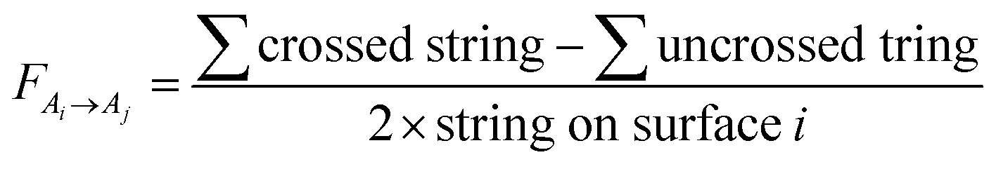 | (47) |
The cross string refers to a diagonal line across the edges of two surfaces, such as the blue lines in Fig. 18. The uncrossed string, on the other hand, refers to the straight line across the edges of two surfaces, such as the red lines in Fig. 18. String on the surface is the line drawn from one edge of the surface to another edge of the same surface. Following eqn (47), the view factors for surface H2 between sky, ground, and rear side of surface H1 (as illustrated in Fig. 18a, b and c respectively) are expressed as:
 | (48) |
 | (49) |
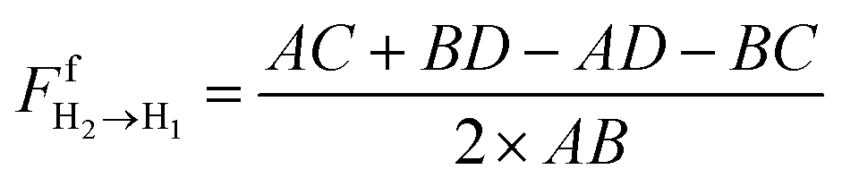 | (50) |
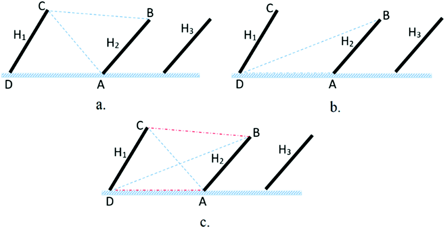 | ||
| Fig. 18 (a) View factor between H2 and sky; (b) view factor between H2 and ground; (c) view factor between H2 and rear side of H1. | ||
Other view factors, e.g., view factor between sky and unshaded ground, and view factor between the shaded ground of front and rear surfaces, are detailed in the respective literature.180 Using the example illustrated in Fig. 18, the total irradiance for front and rear sides of bifacial PV modules within the first row (designated as surface H2)180 is expressed as:
 | (51) |
 | (52) |
 is the global irradiance on surface H2. For modules within the middle row, eqn (51) and (52) are modified to include the reflected irradiance from shaded and unshaded ground:
 | (53) |
 | (54) |
 is the global irradiance on the rear side of surface H1.
The derivations of diffuse and ground-reflected irradiances for the front and rear sides of the bifacial PV module are based on the assumption that both components are isotropic, i.e., uniform over the skydome.164 Also, global irradiance on the rear side of surface H1 does not equal that on the front side of surface H1. Depending on the given time, sun position, and distance between rows, the ground might be partially or fully shaded. If the ground is fully shaded, the third term in eqn (52)–(54) is assumed to be zero. The results163 concluded that the contribution of reflected irradiance from adjacent rows could be omitted. Its contribution is less than the ground-reflected irradiance because PV modules are coated with an anti-reflecting (AR) layer. The module reflectivity is therefore reduced to only a few percent. Furthermore, the cross-string-based approach lacks the consideration of direct and diffuse reflection losses.
4.1.3.1. Empirical formulae. Rather than calculating rear irradiance directly, empirical models are simplified analytical approximations based on measurements or simulations, taking into consideration a more limited set of variables to calculate an approximate bifacial gain per year. Castillo-Aguilella et al.182 developed a simple empirical expression for bifacial gain that depends on tilt angle, β, ground clearance, h, and albedo, α:
| BGE (%) = 0.317 per degree × β + 12.145 m−1 × h + 0.1414 per % × α | (55) |
 | ||
| Fig. 19 Low-tilt, high-albedo (commercial rooftop) rear irradiance gain. 1-Up landscape over 0.62 albedo rooftop. Reprint from ref. 228. Permission granted by the author. | ||
A second empirical model is presented here based on system-level ray-trace modelling. The Kutzer model183 is designed for system-level approximations, and it includes row self-shading effects. The empirical model depends on two geometric factors: ground clearance h and the row-to-row spacing r. Four empirical factors are used in the equations, along with the fractional albedo and module bifaciality:
 | (56) |
Again, BGE [%] is the additional bifacial energy gain in per cent, relative to a monofacial module; and r is the row-to-row spacing normalised by the module table chord length. The ground clearance h is also normalised by the module table chord length. Tilt angle variations between 10° and 30° were found to be of minimal effect for the bifacial gain. Therefore, the tilt angle is not included in eqn (57).
A comparison of these two empirical models is plotted versus height, h, in Fig. 19, compared with results from Marion et al.176 and PVsyst.184 Although it is not capable of capturing latitude-specific or climate-specific effects, the Kutzer model does appear to match closely with more detailed system modelling results for mid-latitude, equator-facing systems.
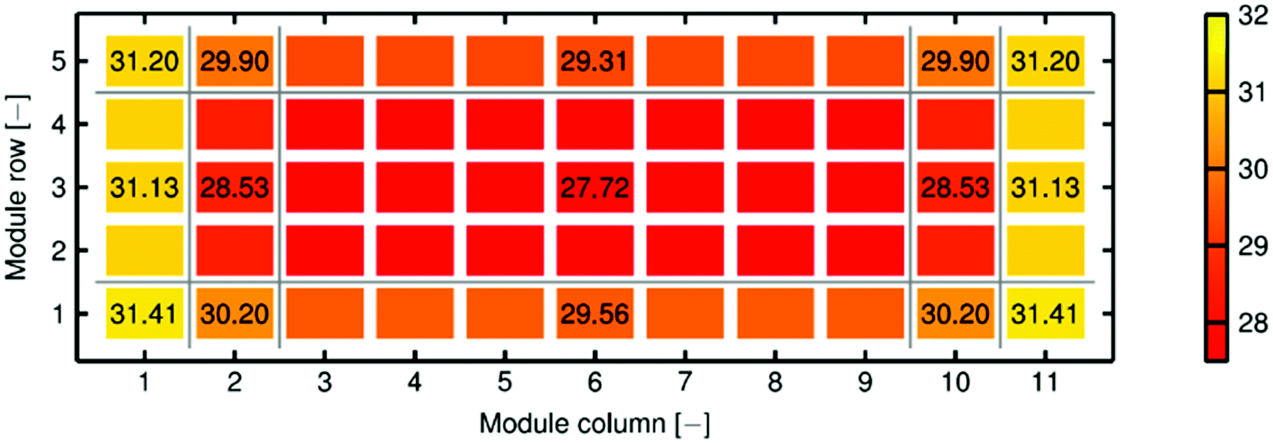 | ||
| Fig. 20 Bifacial gain for each module. Reprint from ref. 165. Licensed under CC BY-NC-ND. | ||
Matlab was used by Hansen et al.164 to integrate eqn (43) for calculation of view factors and rear-side irradiance received by each cell in an array. Modelling of ground-reflected irradiance for shaded and unshaded regions follows eqn (44). The modelling results are illustrated in Fig. 21. The amount of irradiance incident on the cells at the array's edges is higher than that on the cells at the array's centre. The irradiance variation is as much as 10% or higher within the module and among modules. The computation time for four modules at 40 sun positions, according to the authors, is around one minute. For such a short computation time, the simplified 2D view factor model might lose its competitive advantage over the three-dimensional model in simulating small-scale bifacial PV systems with fewer modules and arrays. However, as the computation time scales with the number of modules (cells) and arrays, the 2D model appears to be computationally feasible for modelling the annual performance yield of larger bifacial PV power plants.
 | ||
| Fig. 21 Variation of rear-side irradiance for four modules in a single row. Reprint from ref. 164. Copyright 2016, IEEE. | ||
An updated algorithm185 was proposed to reduce the computation time by omitting the re-calculation of view factor for each reflecting grid surface at each time step. The computation efficiency was further improved when GPU parallelisation was adopted. The simulation model has an accuracy of approximately ±10% for all sky conditions.
4.1.5.1. Single-axis tracking system. Also known as the horizontal single axis tracker (HSAT), a single-axis tracker rotates along the North–South axis, tilts towards the east in the morning and west in the afternoon (as shown in Fig. 22).165,186,187 The optical model is extended to take into consideration the sun position at each time step for a specific period. The following expressions187 describe the example of tracking the sun position:
| tanβtracker = tanθz·[cosγtracker − cosγs] | (57) |
| γtracker = −90° if γs ≤ 0° | (58) |
| γtracker = 90° if γs ≥ 0° | (59) |
 | ||
| Fig. 22 Illustration of a horizontal single axis tracker (HSAT). | ||
Overall, bifacial PV systems equipped with single-axis trackers provide higher energy yields165 and lower LCOE187 (especially in regions near the Equator) as compared to the fixed tilt monofacial or bifacial PV system. However, further analysis of other parameters such as annual seasonality, level of diffuse irradiance and albedo187 are needed before LCOE and yield gains are confirmed. In particular, high ground coverage ratio (GCR) and low albedo natural ground cover tend to reduce the available bifacial energy gain. Available annual rear versus front irradiance levels on the order of 8–12% can be expected for HSAT systems, depending on the particulars of the installation.189
4.1.5.2. Shading effect on beam irradiance. The interference of inter-row shading on the beam irradiance incident on the surface of PV modules is excluded in most bifacial PV performance modelling approaches, except in the study conducted by Appelbaum.163 Based on the inter-row shading investigation190–192 presented by Appelbaum and his colleagues, the length, Ls, and height, Hs, of the shadow (as shown in Fig. 23) cast on the modules (arrays) were determined by:163
 | (60) |
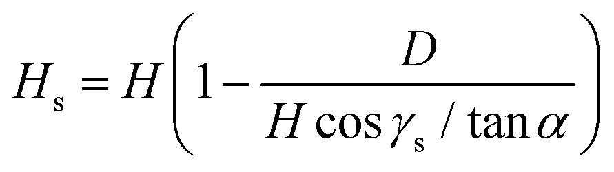 | (61) |
 | (62) |
 | ||
| Fig. 23 Partially-shaded front surface of the middle and third rows. | ||
If the modules (arrays) are not shaded, the above expression becomes 1. For vertically mounted modules, the reduction of beam irradiance is more significant than tilted modules because the height of modules from the ground is higher, thereby casting a longer shadow on the modules behind.163
4.1.5.3. Variation of albedo. As most of the modelling approaches assume uniform and constant albedo across the whole underlying ground, given that the ground area beneath the module and corresponding variation of albedo are small, the assumption might not hold for a long simulation period and large ground area with varying terrain and geographical conditions. According to Chiodetti et al.,193 the daily variation of albedo under clear sky conditions reaches 25% for the concrete floor and 60% for grass, which is determined by the wetting of the concrete floor and grass conditions (dry in the summer/drought or wet after raining). It has also been shown that incorrect albedo values result in underestimation of the annual power output, for as much as 10.5% for vertically-mounted PV modules.194 Therefore, accurate methods for parametrisation of albedo is required, such as the simplified variation albedo model proposed by Chiodetti et al.193 As presented by Brennan et al.,194 the spectrally-responsive albedo is more accurate than the spectrally integrated albedo. It accounts for the spectral responsiveness of the PV module surface and material, and the difference in the mismatch factor between global and ground-reflected irradiance.
4.1.5.4. Rear-side shading. The effect of rear-side shading was evaluated empirically by Riley et al.195 to formulate a model that includes the impact of obstruction (caused by supporting racks, structures or junction box) on the rear-side irradiance. The empirical evaluation was conducted by measuring the I–V curves at different obstruction size, the orientation of obstruction concerning cell string and the distance of the obstacle from the rear side. The expression for a reduction in Pmpp, designated as Dobs, is given by:
| Dobs = −Irear × BiFiPmax × Coverage Ratio | (63) |
Coverage Ratio refers to the ratio between the obstruction size and module's active area. The definition of BiFiPmax is in Section 3.2.1. A scaling factor for eqn (63) is required to represent the impact of the distance of obstruction from the rear side. A simplified version was proposed by Hansen et al.:196
| Pmpp = Pmpp,noobstruction(1 − kobs × Aobs/Amod) | (64) |
4.2. Electrical model
Generally, the calculation of a PV module's electrical output is based on either a single-diode197–199 or a two-diode200–202 equivalent circuit model of a single PV cell. As mentioned in the review paper presented by Chin et al.,203 the single-diode model is inferior as compared to the two-diode model because it neglects the effect of recombination current loss in the depletion region. Furthermore, the accuracy of the single-diode model is severely impacted by temperature variations and at low irradiance, particularly in proximity to open-circuit voltage.201,204 Instead, the two-diode model includes the recombination current loss, which generates more precise results at low irradiance conditions.The two-diode model is illustrated in Fig. 24; its I–V relationship is expressed as:202
 | (65) |
 | ||
| Fig. 24 Circuit diagram of a two-diode model for PV cells. | ||
Several simplifications were proposed in attempting to solve the equation. Commonly, N1 and N2 are assumed as 1 and 2, respectively. However, the validity of this approach has not been proven. In their paper, Salam, Ishaque, and Taheri201 proposed simplified equations to determine Iph, I01, I02, N1, and N2 and calculated Rs and Rp using the iteration method. Suckow et al.200 described a curve fitting algorithm for fitting the I–V characteristics and determining all parameters. In their algorithm, only the ideality factor of the first diode (N1) is treated as 1 and discarded from the fitting process. Yusufoglu et al.103 adopted this curve fitting method by assuming two parallel current sources, which represent the photo-generated current of the front and rear sides of the bifacial PV module; the I–V characteristics of a bifacial PV cell was determined via the methods described in Section 3.1. The assumption is valid given that the short-circuit current corresponds linearly to the incident irradiance, a phenomenon that has been thoroughly discussed in Section 3. Subsequently, the photo-generated current of the rear side is scaled according to the irradiance level of the rear side.
Janssen et al.145 scaled the total short-circuit current using eqn (66) and I01, I02, and Rs using eqn (67):
 | (66) |
 | (67) |
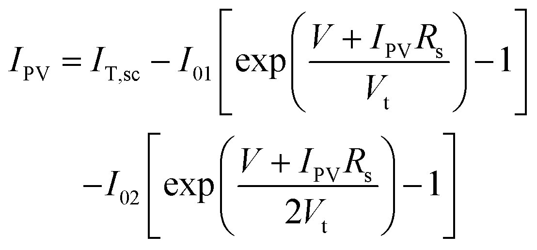 | (68) |
Finally, the electrical outputs of a PV module can be determined by including Ns, which is the number of cells connected in series, into Vt in eqn (65), then multiplying eqn (65) with Np, the number of parallel connected cells:
| IPV,module = IPV × Np | (69) |
4.3. Thermal model
The thermal model calculates the steady-state cell (module) temperature, which is required for correcting the electrical outputs in the electrical model. Yusufoglu et al. and Shoukry et al. used the nominal operating cell temperature (NOCT) formula to account for the temperature effect. In their example, the TNOCT for a bifacial PV module is 47 °C, two degrees higher than that for a monofacial PV module.156Janssen et al. adapted the equation from PVsyst,205 which is based on the module temperature model proposed by Faiman.206 The equation is given as:
 | (70) |
| Ubi = Uc + Uv·νwind | (71) |
Typical values of Uc and Uv, as indicated by PVsyst, are 25 W m−2 K−1 and

 | (72) |
The first term on the right side of the equation calculates the module temperature. GPOA refers to the plane of array irradiance, which should include irradiance on both sides of a bifacial PV module. ΔT represents the difference between the module and cell temperatures. GSTC is the reference irradiance (1000 W m−2). Parameters a and b depend on the module construction, materials, and mounting configuration. Representative values can be obtained in the respective ref. 207.
Correspondingly, Iph, I01, and I02 in eqn (65) become:197,201
 | (73) |
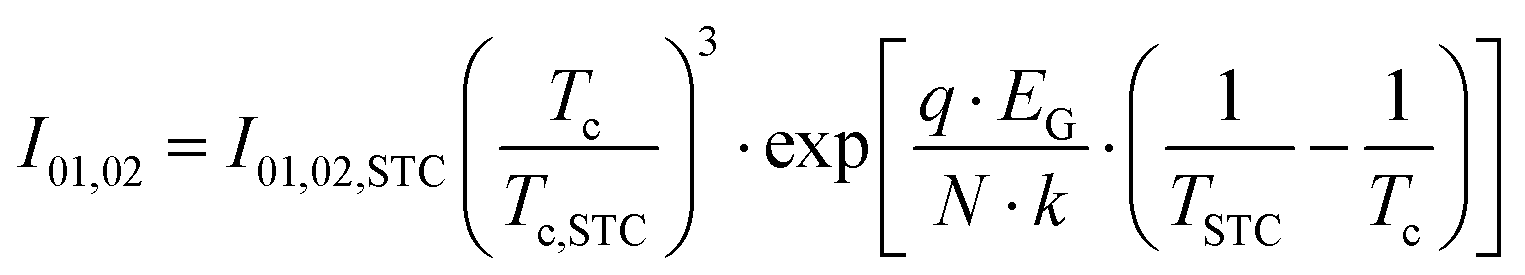 | (74) |
Up to this point, the thermal models do not consider the thermal response time of PV modules. The thermal response time becomes significant when irradiance fluctuates rapidly within a short period and at a small time step (e.g., 1 min).208 The variation of PV modules’ temperature lags behind the changes in irradiance levels under such conditions. Therefore, for performance simulation under short duration, such as the calculation of hourly energy yield with 1 min step change, comprehensive thermal models such as those proposed by Jones and Underwood,208 Armstrong and Hurley,209 and Hayes and Ngan210 should be adopted and modified to accommodate bifacial PV modules.
4.4. Power output and annual energy yield
The DC or AC power output for bifacial PV modules or systems could be determined from the current and voltage values obtained using the electrical model. The annual energy yield (AEY) totals the calculated power output for a given time resolution in a single year. The bifacial gain (BG) reflects the additional energy gain of bifacial PV modules over the monofacial PV modules. AEY and BG are expressed as:100 | (75) |
 | (76) |
Other bifacial PV performance metrics, namely the performance ratio, normalised efficiency, performance index, etc. could be obtained subsequently. The definition and equation of these performance metrics could be easily retrieved from the available literature.
Instead of using the two-diode model coupled with temperature correction, Shoukry et al. carried out an alternative method to calculate the module power output. The method combines the short-circuit current and open-circuit voltage of both sides of bifacial PV based on the model proposed by Singh et al.,109 assuming a linear dependency of Isc and logarithmic dependency of Voc on the incident irradiance. Then power output, AEY, is calculated as:
| Pmpp = FF·Voc,bi·Isc,bi[1 + Kmpp·(Tm − 25 °C)] | (77) |
 | (78) |
 | (79) |
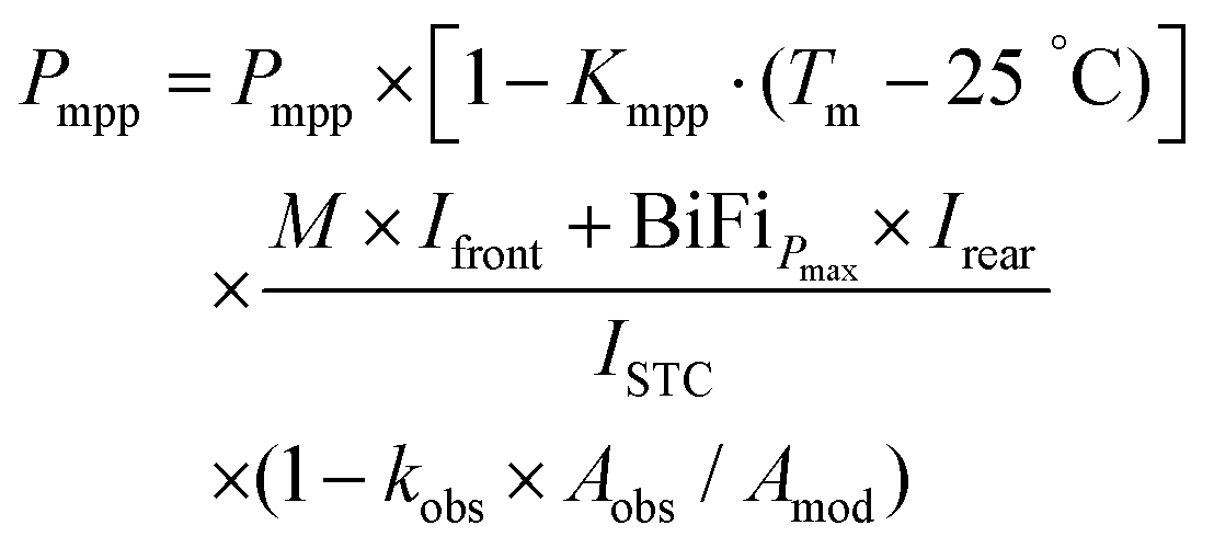 | (80) |
The authors assumed, for simplicity, that M was one since the reference cells and module under test had similar reflection, spectral response, and soiling conditions. A more formal treatment of M would include calculations of reflection losses and spectral mismatch (relative to the irradiance reference). Khoo et al.160 described one such approach to these formulations.
Consensus should be reached in the scientific community to standardise the definitions of energy yield and bifacial gain, as well as other related performance metrics for bifacial PV devices to avoid confusion and misinterpretation. A complete modelling of the bifacial PV system should also include the variations or losses incurred during the conversion and inversion of DC power and transmission to the grid, as shown in Fig. 25. The available models for the monofacial PV system to simulate these variations and losses could be applied to a bifacial PV system. Therefore this review paper does not elaborate on these models.
 | ||
| Fig. 25 Variations and losses incurred along the transfer of electrical power from the bifacial PV module to the grid. | ||
4.5. Levelised cost of energy (LCOE) calculations
Levelised cost of energy (LCOE) for a bifacial PV system allows a fair comparison with systems of different energy sources, operating lifespan, capital cost, and capacities.211 It calculates the present value of the total cost for producing the energy over the proposed operating period, which is described as below:212 | (81) |
Darling et al. proposed an LCOE equation in their study of the assumptions and uncertainties of input variables for LCOE calculation, which was found to be representative and inclusive.213,214 The proposed cost structure is slightly different from eqn (81). It is the project cost without the investment tax or grant, plus the present value of loan payment and annual operation cost, and minus the tax benefit of depreciation, interest paid and residual value. The energy production is the present value of the PV system output that factors in the expected annual degradation. The details of the formula can be read in the references. Overall, the project costs should encompass incurred spending for PV modules, acquirement of land, legal and license processing fees, insurances, civil works, mechanical and electrical installation. The module cost is correlated with the type of PV cell, throughput, interconnection, and other factors, but not depending on efficiency alone.215 On the other hand, the cell production cost is primarily decided by cell processing steps and improvement of efficiency. The cost reduction of new cell technology could be achieved by simultaneously reducing the processing steps and increasing efficiency.216 Fertig et al. studied the cell and module production costs for two bifacial cell structures: PERT and BOSCO (both sides collecting and contacted) in comparison to two monofacial cell structures.217 It shows that the cost reduction of the module with the BOSCO cell structure increases with reducing feedstock price. However, the study also concludes that bifacial illumination could lessen the module cost significantly and outperform the monofacial cell structures, regardless of the feedstock price.
During the operation period, the available solar irradiance, followed by the energy production, depending on the weather forecast and historical weather data. Historical weather data which are longer than ten years should accurately project the future trend, but it might not be true if the weather pattern is significantly altered, e.g., due to global warming. Regarding the system degradation, the glass/glass bifacial PV module structure provides additional protection against the humid environment.39 However, inverters are vulnerable in the same working environment, unless they are specially designed to resist humidity. The system degradation rate is typically less than 1%.212
Singh and Singh218 suggested that equated loan payment (a constant amount of loan is paid for each year) results in higher LCOE for the base year. Instead, a long-term graduated loan payment with the escalation in loan instalments which accounts for the useful life of the PV system (instead of the warranty period of 25 years) and reflects the inflation in the electricity price should be accepted. The annual operation cost depends on a variety of factors, such as the module cleaning frequency or requirement of replacing faulty inverters or wirings. For PV power plants that are located in desert or arid areas, the PV modules require frequent cleaning to maintain energy production. The operation cost might increase over the years as most components degrade.
Other financial parameters such as discount rate, tax rate or subsidy vary according to the country's energy policies and financial regulations imposed on the power plant projects. Some countries introduce a “cap and trade” carbon emission trading scheme, which is beneficial for the PV power plant. In contrast, a daunting economic forecast reduces subsidy or tax credit for the renewable energy sector. Improved certainty for these financial parameters relies on the involvement of government agencies, for instance, economic development agency, central bank or energy policy planning unit.
The challenges of LCOE calculation lie with the assumptions associated with each input parameter. LCOE varies considerably in relation to the input assumptions.214,219 Projects are at increased risk if unrealistic input assumptions are used, such as the projects in Spain where overly optimistic assumptions for module failure rates and other performance parameters were accepted.214 To acknowledge the uncertainties carried by those assumptions, Darling et al.214 suggested the LCOE be calculated using input parameter distributions. Instead of a single LCOE value, a probability distribution of LCOE values is presented. Two reports released by the International Energy Agency, entitled “Technical Assumptions Used in PV Financial Models, Review of Current Practices and Recommendations”220 and “Uncertainties in PV System Yield Predictions and Assessments”,221 provide relevant references for economics and financial models of PV systems, plus the uncertainties of input parameters required for LCOE estimation.
4.6. Modelling software
Lo et al.222 combined the capabilities of three simulation software: RADIANCE, SMART, and PC1D to model and optimise the performance of a bifacial PV module. The function of RADIANCE has been explained in Section 4.1.2.2. Developed by Gueymard et al., SMART is an open-source tool for simulating the solar irradiance spectrum based on the given inputs such as geographical location, time, and local atmospheric parameters. The output from RADIANCE and SMART were imported into PC1D, which executes the electrical and thermal model. The process is summarised in Fig. 26. | ||
| Fig. 26 Flowchart of the integrated simulation tool. Reprint from ref. 222. Copyright 2015, Elsevier. | ||
• PV_Lib Toolbox
• bifacial_radiance
• bifacialvf
Developed at Sandia National Laboratories, the PV_Lib Toolbox224 includes a set of coded functions which are available in Matlab and Python. The functions are categorised into four groups,225 namely the time and location functions, irradiance and atmospheric functions, irradiance translation functions, and photovoltaic system functions. Example scripts are also provided to the users for practising and familiarising themselves with the modelling of a complete PV system. Nevertheless, the toolbox does not currently contain specific functions for bifacial irradiance simulation.
Alternatively, both developed by NREL and available only in Python, bifacial_radiance and bifacialvf allow users to simulate rear-side irradiance.226 Bifacial_radiance provides wrapper functions to facilitate the use of RADIANCE for bifacial PV performance simulation. On the other hand, bifacialvf, based on a study performed by Marion et al.,176 simulates the 2D view factor model assuming an infinitely long array. The details for bifacialvf have been discussed in Section 4.1.3. The comparison of outdoor-measured and simulated values using bifacial_radiance and bifacialvf227 is given in Table 3. For the rear side irradiance ratio during sunny and cloudy periods, both models match closely to the measured values. As compared to bifacial_radiance, bifacialvf produces lower bifacial performance gain. Reasons for that are not explained in the literature. Validation of models with varying row height, row spacing, and edge effect was also carried out to improve the match of simulated and measured data.228
| Outdoor-measured | NREL VF (bifacialvf) | NREL raytracing (bifacial_radiance) | |
|---|---|---|---|
| Rear side irradiance ratio (sunny day) | 17.4% | 17.7% | 16.4% |
| Rear side irradiance ratio (cloudy day) | 14.2% | 14.1% | 14.7% |
| Bifacial performance gain | 8.2% | 7.0% | 7.9% |
Fig. 27 (left) shows the section for the bifacial PV system configuration. Users are required to configure the bifacial PV module, inverter, number of modules in series and number of strings. Users could also choose or input new bifacial PV modules in the databases, including the STC bifaciality factor of the module (if known). Basic parameters for bifacial PV system simulation under fix rack or horizontal single-axis tracking, e.g., ground albedo, structure shading factor, and mismatch loss factor are configured in the “General Simulation Parameters” dialogue box (as shown in Fig. 27, right). The dialogue box of “unlimited sheds” and “unlimited trackers” 2D models are shown in Fig. 28 (left) and (right), respectively. Inside the dialogue box, sheds parameters, e.g. plant tilt/azimuth, pitch, shed width, and height above ground, as well as ground albedo, are configured. Users can observe the drawing (with animation) of the sheds, ground irradiance behaviour (beam, diffuse acceptance, and ground re-emission).184 Ground irradiance for some specified dates and daily irradiance for each month could also be chosen and evaluated. The default loss factors currently in PVSyst include 30% due to the ground albedo, 5% due to the structure shading factor, and 10% due to the mismatch loss factor. These values should be adjusted deliberately based on the specific situation being considered – appropriate numbers can vary considerably by the application.
 | ||
| Fig. 27 Bifacial PV system configuration in PVsyst (left); selection of “unlimited sheds” and “unlimited trackers” 2D model under “General Simulation Parameters” dialog box (right). Print-screened from ref. 230. | ||
 | ||
| Fig. 28 “Unlimited sheds” 2D model dialog box (left); “unlimited trackers” 2D model dialog box (right). Print-screened from ref. 230. | ||
5. Conclusion
The prospect of bifacial PV technology is promising. Despite that, hurdles arising from the characterisation methods, standards, and the energy prediction models pose the most significant challenges to the sustainable penetration of bifacial PV devices into the market. In this review paper, the state-of-the-art bifacial PV performance characterisation and energy simulation modelling are presented. The draft technical specification – IEC 60904-1-2 – requires further refinement, in particular, the procedures for a single illumination source to confine unwanted illumination and properties of the non-reflected material behind the bifacial PV module.Upon finalisation of the draft, inter-lab comparisons of the characterisation results using a single simulator are essential to assess reproducibility and identify areas for improvement. Furthermore, the uncharted simultaneous illumination measurements using two solar simulators necessitate a further experimental investigation. The representativeness of energy rating as the performance indicator for bifacial PV modules is evident, for reasons mentioned in the previous sections. It is therefore vital to produce and popularise an energy rating standard for bifacial PV devices, following the draft standard – IEC 61853 – for energy rating of monofacial PV modules.
Moreover, standards which are similar to IEC 61829 and IEC 61724, or related to the outdoor evaluation of energy production for bifacial PV systems, remain unavailable. Therefore, it is necessary to establish such evaluation procedures to support the performance monitoring and analysis after the successful deployment of large-scale bifacial PV power plants. The international standard for spectral responsivity measurement of PV modules (IEC 60904-8) should also include bifacial PV modules. It is widely assumed that spectral responsivity should be measured on both sides of bifacial PV modules. As a consequence, the spectral mismatch should be evaluated on both sides as well. Correspondingly, a standard spectral albedo should be defined.
Lastly, deciphering the physics of rear-side irradiance remains the priority in the development of performance simulations. Other real-world phenomena which impact the bifacial PV performance, such as the PID and soiling for different outdoor conditions, should also be included in the simulation model. Parameters and input variables, for example, thermal losses, have to be clearly understood and quantified, as compared to the current trend in which many of them are not applied with satisfactory accuracy. Ultimately, the accuracy and consistency of simulation results will have to be maximised to reinforce the confidence of all stakeholders in the PV community, especially investors of large-scale bifacial PV power plants, on using simulation models for energy production and cost estimation. More international collaborations such as the one pioneered by PV Performance Modelling Collaborative (PVPMC) should be developed to offer a platform for improving the performance modelling and analysis.
Conflicts of interest
There are no conflicts to declare.Acknowledgements
The Solar Energy Research Institute of Singapore (SERIS) is a research institute at the National University of Singapore (NUS). SERIS is supported by the National University of Singapore (NUS), National Research Foundation Singapore (NRF) and the Singapore Economic Development Board (EDB).References
- R. Kopecek and J. Libal, Nat. Energy, 2018, 3, 443–446 CrossRef.
- N. Eisenberg, L. Kreinin, N. Bordin, A. Karsenty and A. Drori, Presented at the Bifi PV Workshop, Konstanz, Germany, 2012.
- T. Nordmann, T. Vontobel and R. Lingel, Proceedings of the 28th European PV Solar Energy Conference, 2013, pp. 4797–4799.
- K. Sugibuchi, N. Ishikawa and S. Obara, Proceedings of the 28th European Photovoltaic Solar Energy Conference, 2013, pp. 4312–4317.
- A. Hauser, A. Richter and S. Leu, Cell and module design from the LCOE perspective, 2014.
- P. Grunow, Presented at the Bifi PV Workshop, Konstanz, Germany, 2012.
- M. Hiroshi, US Pat., 3278811, 1966 Search PubMed.
- D. M. Chapin, C. S. Fuller and G. L. Pearson, J. Appl. Phys., 1954, 25, 676–677 CrossRef CAS.
- R. Guerrero-Lemus, R. Vega, T. Kim, A. Kimm and L. E. Shephard, Renewable Sustainable Energy Rev., 2016, 60, 1533–1549 CrossRef CAS.
- I. Chambouleyron and Y. Chevalier, Photovoltaic Solar Energy Conference, 1977, pp. 967–976.
- A. Luque, J. M. Ruiz, A. Cuevas, J. Eguren and M. G. Agost, Photovoltaic Solar Energy Conference, 1977, pp. 269–227.
- A. Luque, A. Cuevas and J. M. Ruiz, Sol. Cells, 1980, 2, 151–166 CrossRef.
- A. Cuevas, A. Luque, J. Eguren and J. Del Alamo, Sol. Cells, 1981, 3, 337–340 CrossRef.
- A. Cuevas, A. Luque, J. Eguren and J. del Alamo, Sol. Energy, 1982, 29, 419–420 CrossRef.
- T. Nordmann, T. Vontobel and L. Clavadetscher, Presented at the Bifi PV Workshop, Konstanz, Germany, 2012.
- R. Hezel, Prog. Photovoltaics Res. Appl., 2003, 11, 549–556 CrossRef.
- I. Araki, M. Tatsunokuchi, H. Nakahara and T. Tomita, Sol. Energy Mater. Sol. Cells, 2009, 93, 911–916 CrossRef CAS.
- T. Joge, L. Araki, K. Takaku, H. Nakahara, Y. Eguchi and T. Tomita, 3rd World Conference on Photovoltaic Energy Conversion, 2003, pp. 1–4.
- R. Kopecek, Presented at the 2nd Bifi PV Workshop, Chambery, France, 2014.
- I. G. Romijn, Presented at the 3rd Bifi PV Workshop, Miyazaki, Japan, 2016.
- N. Ishikawa and S. Nishiyama, Presented at the 3rd Bifi PV Workshop, Miyazaki, Japan, 2016.
- M. Chiodetti, MS thesis, KTH Royal Institute of Technology, 2015.
- PV-Tech, https://www.pv-tech.org/news/worlds_largest_bifacial_pv_plant_nears_completion_in_chile, accessed 28 December 2017.
- Sunpreme, https://www.prnewswire.com/news-releases/sunpreme-deploys-the-worlds-largest-bifacial-pv-installation-for-a-128-mw-utility-project-in-eastern-us-300325989.html, accessed 11 April 2018.
- Photon.info, https://www.photon.info/en/news/yingli-completed-50-mw-pv-project-shanxi-province-china, accessed 11 April 2018.
- TaiyangNews, http://taiyangnews.info/technology/20-mw-bifacial-solar-system-in-china/, accessed 14 March 2018.
- JSB Market Research, http://www.jsbmarketresearch.com/construction/bp1-guaymas-solar-plant-90-mw-sonora-project-profile, accessed 16 May 2018.
- PV-Tech, https://www.pv-tech.org/news/yingli-green-using-bifacial-modules-in-100mw-topper-runner-project, accessed 17 September 2017.
- PV-Tech, https://www.pv-tech.org/editors-blog/bifacial-technology-was-likely-reason-worlds-lowest-ever-solar-bid-was-reje, accessed 3 December 2017.
- International Technology Roadmap for Photovoltaic (ITRPV) – 2017 Results, http://www.itrpv.net/Reports/Downloads/, accessed 4 June 2018.
- R. Kopecek and J. Libal, PV-Tech, pp. 105–110.
- R. Kopecek and J. Libal, Bifacial Photovoltaics: Technology, Applications and Economics, Institution of Engineering and Technology, 2018.
- T. Dullweber, S. Gatz, H. Hannebauer, T. Falcon, R. Hesse, J. Schmidt and R. Brendel, Prog. Photovoltaics Res. Appl., 2012, 20, 630–638 CrossRef CAS.
- J. Zhao, A. Wang, P. P. Altermatt and M. A. Green, Appl. Phys. Lett., 1995, 66, 3636–3638 CrossRef CAS.
- L. Janßen, M. Rinio, D. Borchert, H. Windgassen, D. L. Bätzner and H. Kurz, Prog. Photovoltaics Res. Appl., 2007, 15, 469–475 CrossRef.
- A. Schneider, C. Gerhards, P. Fath, E. Bucher, R. J. S. Young, J. A. Raby and A. F. Carroll, Conference Record of the Twenty-Ninth IEEE Photovoltaic Specialists Conference, 2002, pp. 336–339.
- J. P. Singh, S. Guo, I. M. Peters, A. G. Aberle and T. M. Walsh, IEEE J. Photovolt., 2015, 5, 783–791 Search PubMed.
- Y. Zhang, J. Xu, Y. Shu, P. Quan, Y. Wang, J. Mao, Y. Gao, C. Fu, Z. Feng, P. J. Verlinden, P. Yang and J. Chu, Proc. 28th Eur. Photovolt. Sol. Energy Conf., 2013, pp. 3123–3126.
- T. M. Walsh, Z. Xiong, Y. S. Khoo, A. a. O. Tay and A. G. Aberle, Energy Procedia, 2012, 15, 388–395 CrossRef.
- W. Luo, Y. S. Khoo, J. P. Singh, J. K. C. Wong, Y. Wang, A. G. Aberle and S. Ramakrishna, IEEE J. Photovolt., 2017, 8, 16–22 Search PubMed.
- W. Luo, P. Hacke, K. Terwilliger, T. S. Liang, Y. Wang, S. Ramakrishna, A. G. Aberle and Y. S. Khoo, Prog. Photovoltaics, 2018, 1–9 Search PubMed.
- T. Söderström, P. Papet and J. Ufheil, Proceedings of the 28th European Photovoltaic Solar Energy Conference, 2013, pp. 495–499.
- S. Braun, G. Hahn, R. Nissler, C. Pönisch and D. Habermann, Energy Procedia, 2013, 38, 334–339 CrossRef CAS.
- J. Dupuis, E. Saint-Sernin, O. Nichiporuk, P. Lefillastre, D. Bussery and R. Einhaus, Conference Record of the IEEE Photovoltaic Specialists Conference, 2012, pp. 3183–3186.
- J. Walter, M. Tranitz, M. Volk, C. Ebert and U. Eitner, Energy Procedia, 2014, 55, 380–388 CrossRef.
- S. Guo, J. P. Singh, I. M. Peters, A. G. Aberle and T. M. Walsh, Int. J. Photoenergy, 2013, 1–8 CrossRef.
- Y. S. Khoo, J. P. Singh and M. H. Saw, Presented at the 3rd Bifi PV Workshop, Miyazaki, Japan, 2016.
- J. P. Singh, Y. Wang and Y. S. Khoo, Presented at the 4th Bifi PV Workshop, Konstanz, Germany, 2017.
- B. B. Van Aken, presented at the 3rd Bifi PV Workshop, Miyazaki, Japan, 2016.
- Sunmodule Bisun protect, https://www.solarworld.de/en/products/sunmodule-bisun-protect/, accessed 11 January 2018.
- M. H. Saw, Y. S. Khoo, J. P. Singh and Y. Wang, Energy Procedia, 2017, 124, 484–494 CrossRef.
- B. B. Van Aken, J. A. M. Van Roosmalen, L. A. G. Okel, I. G. Romijn and G. J. M. Janssen, Proceedings of the 31st European Photovoltaic Solar Energy Conference, 2015, pp. 100–103.
- A. Hübner, A. G. Aberle and R. Hezel, Appl. Phys. Lett., 1997, 70, 1008–1010 CrossRef.
- T. Dullweber, C. Kranz, R. Peibst, U. Baumann, H. Hannebauer, A. Fülle, S. Steckemetz, T. Weber, M. Kutzer, M. Müller, G. Fischer, P. Palinginis and D. H. Neuhaus, Proceedings of the 31st European Photovoltaic Solar Energy Conference, 2015, pp. 341–350.
- A. G. Aberle, S. W. Glunz and W. Warta, Appl. Phys., 1992, 71, 4422–4431 CAS.
- J. Knobloch, A. G. Aberle and W. B. Voß, Eighth E.C. Photovoltaic Solar Energy Conference, 1988, pp. 1165–1170.
- White Paper – Increased Energy Yield Through Bifacial Technology, https://www.solarworld-usa.com/technical-downloads/technical-bulletins, accessed 21 March 2018.
- E. Lohmüller, S. Werner, M. H. Norouzi, S. Mack, M. Demant, S. Gutscher, P. Saint-Cast, M. Hermle, A. Wolf, B. Bitnar, P. Palinginis, H. Neuhaus and M. König, Proceedings of the 33rd European PV Solar Energy Conference, Amsterdam, 2017 Search PubMed.
- J. Zhao, A. Wang and M. A. Green, IEEE Photovoltaic Spec. Conf., 1990, 333–335 CAS.
- N. Ishikawa, Presented at the Bifi PV Workshop, Konstanz, Germany, 2012.
- I. G. Romijn, B. B. Van Aken, J. Anker, P. Barton, A. Gutjahr, Y. Komatsu, M. Koppes, E. J. Kossen, M. W. P. E. Lamers, D. S. Saynova, K. C. J. J. Tool, Y. Zhang-Steenwinkel, P. R. Venema, A. H. G. Vlooswijk, C. Schmitt, H. Kühnlein, N. Bay, M. König and A. Stassen, Proceedings of the 28th European Photovoltaic Solar Energy Conference, 2013, pp. 736–740.
- W. Cai, S. Yuan, Y. Sheng, W. Duan, Z. Wang, Y. Chen, Y. Yang, P. P. Altermatt, P. J. Verlinden and Z. Feng, Energy Procedia, 2016, 92, 399–403 CrossRef CAS.
- Q. Wei, S. Zhang, S. Yu, J. Lu, W. Lian and Z. Ni, Energy Procedia, 2017, 124, 700–705 CrossRef CAS.
- https://www.imec-int.com/en/articles/imec-develops-industry-compatible-screen-printing-process-for-highly-efficient-n-pert-solar-cells .
- L. Kreinin, Presented at the 4th Bifi PV Workshop, Konstanz, Germany, 2017.
- B. Geerligs, Presented at the 5th MWT Workshop, Freiburg, Germany, 2013.
- The BiSoN solar cell, http://www.mega-group.it/megacell/en/the-bison-solar-cell/, accessed 11 February 2018.
- G. Galbiati, H. Chu, V. D. Mihailetchi, J. Libal and R. Kopecek, Presented at the World Conference on Photovoltaic Energy Conversion (WCPEC-7), 2018.
- V. D. Mihailetchi, A. Halm, C. Comparotto, S. Aulehla and R. Kopecek, Presented at the 2nd Bifi PV Workshop, Chambery, France, 2014.
- R. Kopecek and Y. Veschetti, Photovolt. Int., 2015, 26, 32–45 Search PubMed.
- A. Halm, V. D. Mihailetchi, G. Galbiati, L. J. Koduvelikulathu, R. Roescu, C. Comparotto, R. Kopecek, K. Peter and J. Libal, Proceeding of the 27th European Photovoltaic Solar Energy Conference and, 2012, pp. 567–570.
- G. Galbiati, V. D. Mihailetchi, R. Roescu, A. Halm, L. J. Koduvelikulathu, R. Kopecek, K. Peter and J. Libal, IEEE J. Photovolt., 2013, 3, 560–565 Search PubMed.
- I. Cesar, N. Guillevin, A. A. Mewe, P. Spinelli, A. R. Burgers, V. Rosca, L. A. G. Okel, B. J. Geerligs, A. W. Weeber, S. Sawallich and M. Nagel, Energy Procedia, 2017, 124, 834–841 CrossRef.
- A. A. Mewe, P. Spinelli, A. Burgers, G. J. M. Janssen, N. Guillevin, B. Van De Loo, E. Kessels, A. Ylooswijk, B. Geerligs and I. Cesar, Proceedings of the 42nd IEEE Photovoltaic Specialist Conference, 2015.
- M. Taguchi, A. Yano, S. Tohoda, K. Matsuyama, Y. Nakamura, T. Nishiwaki, K. Fujita and E. Maruyama, IEEE J. Photovolt., 2014, 4, 96–99 Search PubMed.
- I. G. Romijn, Presented at the 4th Bifi PV Workshop, Konstanz, Germany, 2017.
- Panasonic HIT history, https://eu-solar.panasonic.net/en/panasonic-hit-sanyo-history.htm, accessed 11 January 2018.
- T. Kinoshita, D. Fujishima, A. Yano, A. Ogane, S. Tohoda, K. Matsuyama, Y. Nakamura, N. Tokuoka, H. Kanno, H. Sakata, M. Taguchi and E. Maruyama, Proceedings of the 26th European Photovoltaic Solar Energy Conference, 2011, pp. 871–874.
- HIT Double Photovoltaic module, http://www.panasonic.com/business/pesna/includes/pdf/eco-construction-solution/HIT_Double_190_Datasheet.pdf, accessed 12 March 2018.
- White Paper – Heterojunction Technology, https://www.meyerburger.com/sg/en/meyer-burger/media/multimedia/publications/article/heterojunction-technology-the-solar-cell-of-the-future/, accessed 4 July 2018.
- S. B. Ghozati, A. U. Ebong, C. B. Honsberg and S. R. Wenham, Sol. Energy Mater. Sol. Cells, 1998, 51, 121–128 CrossRef CAS.
- S. R. Wenham, B. O. Chan, C. B. Honsberg and M. A. Green, Prog. Photovoltaics Res. Appl., 1997, 5, 131–137 CrossRef CAS.
- A. U. Ebong, S. H. Lee, C. Honsberg and S. R. Wenham, Jpn. J. Appl. Phys., Part 1, 1996, 35, 2077–2080 CrossRef CAS.
- P. J. Verlinden, A. W. Blakers, K. J. Weber, J. Babaei, V. Everett, M. J. Kerr, M. F. Stuckings, D. Gordeev and M. J. Stocks, Sol. Energy Mater. Sol. Cells, 2006, 90, 3422–3430 CrossRef CAS.
- K. J. Weber, A. W. Blakers, V. A. Everett and E. Frank, Australian Institute of Energy National Conference – ‘Energy at the Crossroads’, 2006.
- G. G. Untila, T. N. Kost, A. B. Chebotareva, M. B. Zaks, A. M. Sitnikov, O. I. Solodukha and M. Z. Shvarts, Prog. Photovoltaics Res. Appl., 2015, 23, 600–610 CrossRef CAS.
- IEC 60904-1, Edition 2.0, 2006.
- IEC 60904-5, Edition 2.0, 2011.
- IEC 60904-7, Edition 3.0, 2008.
- IEC 60904-8, Edition 3.0, 2014.
- IEC 60904-10, Edition 2.0, 2009.
- IEC 60904-4, Edition 1.0, 2009.
- IEC 60904-2, Edition 3.0, 2015.
- IEC 60904-3, Edition 3.0, 2016.
- IEC 60904-9, Edition 2.0, 2007.
- IEC 61853-1, Edition 1.0, 2011.
- IEC 61853-2, Edition 1.0, 2016.
- J. P. Singh, PhD dissertation, National University of Singapore, 2014.
- G. Razongles, L. Sicot, M. Joanny, E. Gerritsen, P. Lefillastre, S. Schroder and P. Lay, Energy Procedia, 2016, 92, 188–198 CrossRef CAS.
- G. J. M. Janssen, B. B. Van Aken, A. J. Carr and A. A. Mewe, Energy Procedia, 2015, 77, 364–373 CrossRef.
- B. B. Van Aken, M. J. Jansen and N. J. J. Dekker, IEEE 39th Photovoltaic Specialists Conference, 2013, pp. 1610–1614.
- B. B. Van Aken and A. J. Carr, IEEE 40th Photovoltaic Specialist Conference, 2014, pp. 1381–1383.
- U. A. Yusufoglu, T. M. Pletzer, L. J. Koduvelikulathu, C. Comparotto, R. Kopecek and H. Kurz, IEEE J. Photovolt., 2015, 5, 320–328 Search PubMed.
- R. Kopecek and J. Libal, PV-Tech, 2018.
- LG NeON 2BiFacial (LG300N1T-G4), http://www.lg-solar.com/downloads/products/LGE-Data Sheet-LG300N1T-G4-EN-08.2016.pdf, accessed 13 November 2017.
- HIT Double 195, https://www.solarelectricsupply.com/sanyo-195-watt-solar-panel-hip-195da3-517, accessed 27 October 2017.
- MAXIMA GxB 320W Bifacial Module, http://sunpreme.com/wp-content/uploads/2017/10/20171004-Sunpreme-Datasheet-GxB-320T-SM-Bifacial-Module-Rev-1-2.pdf, accessed 27 October 2017.
- L. Kreinin, N. Bordin and N. Eisenberg, Presented at the Bifi PV Workshop, Konstanz, Germany, 2012.
- J. P. Singh, A. G. Aberle and T. M. Walsh, Sol. Energy Mater. Sol. Cells, 2014, 127, 136–142 CrossRef CAS.
- Design Guide for Bifacial Solar Modules, http://atlassolarproducts.com/files/5714/3776/5993/Prism.Design_guide.pdf, accessed 27 October 2017.
- Bifacial Module Models Bi60-362, -368, -375BSTC, https://static1.squarespace.com/static/57a12f5729687f4a21ab938d/t/58cc774837c5819ccd0e5f41/1489794889716/bi60specs.pdf, accessed 3 October 2017.
- A. R. Burgers, Presented at the Bifi PV Workshop, Konstanz, Germany, 2012.
- A. Sitnikov, Presented at the Bifi PV Workshop, Konstanz, Germany, 2012.
- M. Rauer, K. Bothe, C. Comparotto, P. Danzl, M. Debucquoy, N. Enjalbert, J. Hohl-Ebinger, P. Manshanden, Y. Veschetti and J. K. C. Wong, Proceedings of the 32nd European Photovoltaic Solar Energy Conference, 2016, pp. 915–921.
- J. Hohl-Ebinger and W. Warta, Proceedings of the 25th European Photovoltaic Solar Energy Conference, 2010, pp. 1358–1362.
- C. Duran, P. Hering, T. Buck and K. Peter, Proceedings of the 26th European Photovoltaic Solar Energy Conference, 2011, pp. 1550–1554.
- C. Duran, H. Deuser, R. Harney and T. Buck, Energy Procedia, 2011, 8, 88–93 CrossRef.
- J. P. Singh, J. Chai, M. H. Saw and Y. S. Khoo, Jpn. J. Appl. Phys., 2017, 56, 08MD04 CrossRef.
- J. P. Singh, T. M. Walsh and A. G. Aberle, Prog. Photovoltaics Res. Appl., 2014, 22, 903–909 CrossRef.
- M. Ezquer, I. Petrina, J. M. Cuadra and A. R. Lagunas, Proceedings of the 23rd European Photovoltaic Solar Energy Conference, 2013, pp. 1553–1556.
- H. Ohtsuka, M. Sakamoto, M. Koyama, K. Tsutsui, T. Uematsu and Y. Yazawa, Prog. Photovoltaics Res. Appl., 2001, 9, 1–13 CrossRef CAS.
- h.a.l.m. elektronik, http://www.halm.de/en/news/new-cetispv-iuct-bf.html, accessed 11 February 2018.
- K. Ramspeck and A. Metz, Presented at the PV-Seminar at UNSW, 2017.
- C. Deline, S. MacAlpine, B. Marion, F. Toor, A. Asgharzadeh and J. S. Stein, IEEE J. Photovolt., 2017, 7, 575–580 Search PubMed.
- B. Soria, Y. Veschetti, P. Lefillastre and E. Gerritsen, Presented at the Bifi PV Workshop, Konstanz, Germany, 2012.
- C. Comparotto, N. Matthias, L. Popescu, A. Edler, J. Ranzmeyer, T. Klaus, V. D. Mihailetchi, R. Harney, J. Lossen, T. S. Boscke, D. Schar, H. Nussbaumer, T. Baumann, F. P. Baumgartner, M. Noebels, L. Popescu, A. Edler, J. Ranzmeyer, T. Klaus, V. D. Mihailetchi, R. Harney, J. Lossen, T. S. Böscke, D. Schar, H. Nussbaumer, T. Baumann and F. P. Baumgartner, Proceedings of the 29th European Photovoltaic Solar Energy Conference, 2014, pp. 366–372.
- A. G. Montgareuil, L. Sicot, J.-L. Martin, F. Mezzasalma, Y. Delesse and J. Merten, Proceedings of the 24th European Photovoltaic Solar Energy Conference, 2009, pp. 3305–3309.
- G. Corbellini and V. Medici, Presented at the 4th PV Performance Modelling Collaborative Workshop, Cologne, Germany, 2015.
- A. Edler and A. Metz, Presented at the Workshop on Bifacial Photovoltaics Implemented in the Atacama Desert Solar Platform, Antofagasta, Chile, 2015.
- B. Soria, E. Gerritsen, P. Lefillastre and J.-E. Broquin, Energy Sci. Eng., 2016, 4, 52–68 CrossRef CAS.
- M. Bliss, T. R. Betts and R. Gottschalg, Meas. Sci. Technol., 2010, 21, 115701 CrossRef.
- M. Stuckelberger, B. Perruche, M. Bonnet-Eymard, Y. Riesen, M. Despeisse, F. J. Haug and C. Ballif, IEEE J. Photovolt., 2014, 4, 1282–1287 Search PubMed.
- WAVELABS SINUS-220, http://wavelabs.de/wp-content/uploads/Data_sheet_SINUS-220.pdf, accessed 2 December 2017.
- J. P. Singh, T. M. Walsh and A. G. Aberle, Proceedings of the 27th European Photovoltaic Solar Energy Conference, 2012, pp. 3263–3266.
- S. Sciara, S. J. Suk and G. Ford, J. Build. Constr. Plan. Res., 2016, 4, 41 Search PubMed.
- L. Kreinin, N. Bordin, A. Karsenty, A. Drori, D. Grobgeld and N. Eisenberg, Proceedings of the 35th IEEE Photovoltaic Specialists Conference, 2010, pp. 002171–002175.
- DOUBLE PYRANOMETER TYPE 8104, http://www.skypowerinternational.com/uploads/documents/8104eng_open.pdf, accessed 11 November 2017.
- Kipp & Zonen, http://www.kippzonen.com/Product/23/CMA11-Albedometer#.WfqSMWhL-Uk, accessed 11 November 2017.
- SRA01 albedometer, https://www.hukseflux.com/product/sra01-albedometer, accessed 15 November 2017.
- R. Pirazzini, J. Geophys. Res., 2004, 109, 1–15 CrossRef.
- D. Faiman, D. Berman, D. Bukobza, S. Kabalo, I. Karki, B. Medwed, V. Melnichak, E. De Held and H. Oldenkamp, Proceedings of the 3rd World Conference on Photovoltaic Energy Conversion, 2003, vol. 2, pp. 1988–1991.
- IEC TS 60904-1-2 ED1, in draft version at the time of writing, 2018.
- N. Bassi, Presented at the Energy Rating for Photovoltaics: evaluating real-world performance, NPL, UK, 2016.
- V. Fakhfouri, Presented at the 4th Bifi PV Workshop, Konstanz, Germany, 2017.
- G. J. M. Janssen, B. B. Van Aken, A. J. Carr and A. A. Mewe, Energy Procedia, 2015, 77, 364–373 CrossRef.
- D. Berrian, J. Libal and S. W. Glunz, Presented at the 4th Bifi PV Workshop, Konstanz, Germany, 2017.
- Meteonorm, http://www.meteonorm.com/, accessed 11 January 2018.
- Solargis, https://solargis.com/, accessed 11 October 2017.
- PVGIS, http://re.jrc.ec.europa.eu/pvgis/, accessed 11 March 2018.
- Y. S. Khoo, A. Nobre, R. Malhotra, D. Yang, R. Ruther, T. Reindl and A. G. Aberle, IEEE J. Photovolt., 2014, 4, 647–653 Search PubMed.
- R. Perez, R. Stewart, C. Arbogast, R. Seals and J. Scott, Sol. Energy, 1986, 36, 481–497 CrossRef.
- R. Perez, R. Seals, P. Ineichen, R. Stewart and D. Menicucci, Sol. Energy, 1987, 39, 221–231 CrossRef.
- R. Perez, P. Ineichen, R. Seals, J. Michalsky and R. Stewart, Sol. Energy, 1990, 44, 271–289 CrossRef.
- P. Ineichen, O. Guisan and R. Perez, Sol. Energy, 1990, 44, 207–214 CrossRef.
- M. Iqbal, An Introduction to Solar Radiation, Academic Press Canada Ontario, 1983, pp. 295–301 Search PubMed.
- U. A. Yusufoglu, T. H. Lee, T. M. Pletzer, A. Halm, L. J. Koduvelikulathu, C. Comparotto, R. Kopecek and H. Kurz, Energy Procedia, 2014, 55, 389–395 CrossRef.
- POA Ground Reflected, https://pvpmc.sandia.gov/modeling-steps/1-weather-design-inputs/plane-of-array-poa-irradiance/calculating-poa-irradiance/poa-ground-reflected/, accessed 11 November 2017.
- A. Krenzinger and E. Lorenzo, Int. J. Sol. Energy, 1986, 4, 297–319 CrossRef.
- N. Martin and J. M. Ruiz, Sol. Energy Mater. Sol. Cells, 2001, 70, 25–38 CrossRef CAS.
- Y. S. Khoo, J. P. Singh, T. M. Walsh and A. G. Aberle, IEEE J. Photovolt., 2014, 4, 362–367 Search PubMed.
- D. L. King, W. E. Boyson and J. A. Kratochvil, Photovoltaic array performance model, 2004, vol. 8 Search PubMed.
- N. Y. Fathi and A. Samer, J. Sol. Energy Eng. Trans. ASME, 2016, 138, 1–8 Search PubMed.
- J. Appelbaum, Renewable Energy, 2016, 85, 338–343 CrossRef.
- C. W. Hansen, J. S. Stein, C. Deline, S. MacAlpine, B. Marion, A. Asgharzadeh and F. Toor, IEEE 44th Photovoltaic Specialist Conference (PVSC), IEEE, 2017, pp. 1–6.
- I. Shoukry, J. Libal, R. Kopecek, E. Wefringhaus and J. Werner, Energy Procedia, 2016, 92, 600–608 CrossRef.
- U. Gross, K. Spindler and E. Hahne, Lett. Heat Mass Transfer, 1981, 8, 219–227 CrossRef.
- U. A. Yusufoglu, T. M. Pletzer, B. Min, J. van Mölken, B. Litzenburger, S. Pingel, W. Herrmann and H. Kurz, Proceedings of the 28th European Photovoltaic Solar Energy Conference, Paris, 2013, pp. 3203–3206.
- The RADIANCE Lighting Simulation and Rendering System, http://radsite.lbl.gov/radiance/framew.html, accessed 11 January 2018.
- TracePro, https://www.lambdares.com/tracepro/, accessed 11 September 2017.
- Simulate Ray Tracing in Optically Large System with the Ray Optics Module, https://www.comsol.com/ray-optics-module, accessed 11 November 2017.
- Sophomore College Ray Tracing Site, https://cs.stanford.edu/people/eroberts/courses/soco/projects/1997-98/ray-tracing/types.html, accessed 7 January 2018.
- Schorsch.com, http://www.schorsch.com/en/kbase/glossary/raytracing.html, accessed 11 January 2018.
- J. S. Stein, C. W. Hansen and B. Marion, Presented at the 9th PV Performance Modeling and Monitoring Workshop, 2017.
- D. Robinson and A. Stone, The 21st Conference on Passive and Low Energy Architecture, Eindhoven, The Netherlands, 2004, pp. 1–5.
- A. Asgharzadeh, B. Marion, C. Deline, C. Hansen, J. S. Stein and F. Toor, IEEE J. Photovolt., 2018, 8, 798–805 Search PubMed.
- B. Marion, S. Macalpine, C. Deline, A. Asgharzadeh, F. Toor, D. Riley, J. S. Stein and C. W. Hansen, IEEE 44th Photovoltaic Specialist Conference, Washington, DC, 2017 Search PubMed.
- E. A. Sjerps-Koomen, E. A. Alsema and W. C. Turkenburg, Sol. Energy, 1996, 57, 421–432 CrossRef.
- B. Marion, Sol. Energy, 2017, 147, 344–348 CrossRef.
- T. Maor and J. Appelbaum, Sol. Energy, 2012, 86, 1701–1708 CrossRef.
- J. Appelbaum, Renewable Sustainable Energy Rev., 2018, 81, 161–171 CrossRef.
- H. Hottel and A. Sarofin, Radiative Transfer, McGraw Hill, New York, 1967 Search PubMed.
- J. E. Castillo-Aguilella and P. S. Hauser, IEEE Access, 2016, 4, 498–506 Search PubMed.
- M. Kutzer, A. Fülle, A. Jahnke, J. B. H. Hahn, S. Wendt, D. H. Neuhaus, A. Witzig, L. Kunath and U. Stöckli, Symposium Photovoltaische Solarenergie, 2018 Search PubMed.
- PVsyst 6 Help, http://files.pvsyst.com/help/index.html?bifacial_module.htm, accessed 25 November 2017.
- C. W. Hansen, R. Gooding, N. Guay, D. M. Riley, J. Kallickal, A. Asgharzadeh, B. Marion, F. Toor and J. S. Stein, Proceedings of the 44th IEEE Photovoltaic Specialists Conference, 2017.
- M. A. Anoma, D. Jacob, B. C. Bourne, J. A. Scholl, D. M. Riley and C. W. Hansen, Proceedings of the 44th IEEE Photovoltaic Specialists Conference, 2017.
- A. Lindsay, M. Chiodetti, D. Binesti, S. Mousel, E. Lutun, K. Radouane and J. Christopherson, Proceedings of the 32nd European Photovoltaic Solar Energy Conference, 2016, pp. 1610–1617.
- M. Libra and V. Poulek, Physical Methods in Agriculture, Springer US, Boston, 2002, pp. 83–104 Search PubMed.
- S. A. Pelaez, C. Deline, P. Greenberg, J. S. Stein and R. K. Kostuk, 7th World Conference on Photovoltaic Energy Conversion, 2018.
- J. Bany and J. Appelbaum, Sol. Cells, 1987, 20, 201–228 CrossRef.
- J. Appelbaum and J. Bany, Sol. Energy, 1979, 23, 497–507 CrossRef.
- D. Weinstock and J. Appelbaum, J. Sol. Energy Eng., 2004, 126, 898 CrossRef.
- M. Chiodetti, A. Lindsay, P. Dupeyrat, D. Binesti, E. Lutun, K. Radouane and S. Mousel, Proceedings of the 32nd European Photovoltaic Solar Energy Conference, 2016, pp. 1449–1455.
- M. P. Brennan, A. L. Abramase, R. W. Andrews and J. M. Pearce, Sol. Energy Mater. Sol. Cells, 2014, 124, 111–116 CrossRef CAS.
- D. Riley, C. W. Hansen, J. S. Stein, M. Lave, J. Kallickal and B. Marion, Proceedings of the 44th IEEE Photovoltaic Specialists Conference, 2017.
- C. W. Hansen, D. M. Riley, C. Deline, F. Toor and J. S. Stein, Proceedings of the 33rd European PV Solar Energy Conference, 2017.
- M. Jazayeri, S. Uysal and K. Jazayeri, High Capacity Optical Networks and Emerging/Enabling Technologies, IEEE, 2013, pp. 44–50.
- A. A. EL Tayyan, Turk. J. Phys., 2013, 37, 121–131 Search PubMed.
- F. González-Longatt, Ii Cibelec, 2005, pp. 1–5.
- S. Suckow, T. M. Pletzer and H. Kurz, Prog. Photovoltaics Res. Appl., 2014, 22, 494–501 CrossRef.
- Z. Salam, K. Ishaque and H. Taheri, Joint International Conference on Power Electronics, Drives and Energy Systems, PEDES, 2010, vol. 1, pp. 1–5.
- A. V. Pavan Kumar, A. M. Parimi and K. Uma Rao, IEEE International Conference on Advanced Communications, Control and Computing Technologies, IEEE, 2014, pp. 68–72.
- V. J. Chin, Z. Salam and K. Ishaque, Appl. Energy, 2015, 154 Search PubMed.
- N. Mohamed, A. Alrahim, N. Z. Yahaya and B. Singh, IEEE International Conference on Control System, Computing and Engineering, 2013, pp. 210–214.
- PVsyst 6 Help, http://files.pvsyst.com/help/index.html?thermal_loss.htm, accessed 11 January 2018.
- D. Faiman, Prog. Photovoltaics Res. Appl., 2008, 16, 307–315 CrossRef CAS.
- Sandia Cell Temperature Model, https://pvpmc.sandia.gov/modeling-steps/2-dc-module-iv/cell-temperature/sandia-cell-temperature-model/, accessed 11 January 2018.
- A. D. Jones and C. P. Underwood, Sol. Energy, 2001, 70, 349–359 CrossRef CAS.
- S. Armstrong and W. G. Hurley, Appl. Therm. Eng., 2010, 30, 1488–1495 CrossRef.
- W. Hayes and L. Ngan, IEEE J. Photovolt., 2015, 5, 238–242 Search PubMed.
- DOE Office of Indian Energy, https://energy.gov/sites/prod/files/2015/08/f25/LCOE.pdf, accessed 11 April 2018.
- K. Branker, M. J. M. Pathak and J. M. Pearce, Renewable Sustainable Energy Rev., 2011, 15, 4470–4482 CrossRef.
- https://www.solarserver.com/solar-magazine/solar-point-of-view/solar-point-of-view/solar-perspectives-what-is-inside-your-lcoe-assumptions.html, accessed 11 February 2018.
- S. B. Darling, F. You, T. Veselka and A. Velosa, Energy Environ. Sci., 2011, 4, 3133–3139 RSC.
- M. A. Green, Prog. Photovoltaics Res. Appl., 2005, 13, 85–87 CrossRef.
- N.-P. Harder, 21st Workshop on Crystalline Silicon Solar Cells and Modules.
- F. Fertig, S. Nold, N. Wöhrle, J. Greulich, I. Hädrich, K. Krauß, M. Mittag, D. Biro, S. Rein and R. Preu, Prog. Photovoltaics Res. Appl., 2016, 24, 800–817 CrossRef.
- P. P. Singh and S. Singh, Renewable Energy, 2010, 35, 563–569 CrossRef.
- The Drivers of the Levelized Cost of Electricity for Utility-Scale Photovoltaics, sunpowercorp.com, accessed 2 August 2018.
- M. Richter, C. Tjengdrawira, J. Vedde, M. Green, L. Frearson, B. Herteleer, U. Jahn, M. Herz, M. Köntges, B. Stridh, K. Berger, J. Eckhard, D. Moser, G. Belluardo and N. Reich, Technical Assumptions Used in PV Financial Models. Review of Current Practices and Recommendations. IEA-PVPS, Report IEA-PVPS T13-08:2017.
- C. Reise, B. Müller, D. Mose, G. Belluardo, P. Ingenhoven, A. Driesse, G. Razongles and M. Richter, Uncertainties in PV System Yield Predictions and Assessments. IEA-PVPS, Report IEA-PVPS T13-12:2018.
- C. K. Lo, Y. S. Lim and F. A. Rahman, Renewable Energy, 2015, 81, 293–307 CrossRef.
- PV Performance Modeling Collaborative, https://pvpmc.sandia.gov/, accessed 11 December 2017.
- PV_LIB Toolbox, https://pvpmc.sandia.gov/applications/pv_lib-toolbox/, accessed 11 December 2017.
- J. S. Stein, Conference Record of the IEEE Photovoltaic Specialists Conference, 2012, pp. 3048–3052.
- Bifacial Open Source Software, https://pvpmc.sandia.gov/pv-research/bifacial-pv-project/, accessed 11 September 2017.
- S. Macalpine, C. Deline and B. Marion, Presented at the 8th PV Performance Modeling and Monitoring Workshop, 2017.
- C. Deline, B. Marion, S. Macalpine, J. S. Stein, F. Toor and S. Ayala, Presented at the 4th Bifi PV Workshop, Konstanz, Germany, 2017.
- A. Mermoud and B. Wittmer, Presented at the 10th PV Performance Modeling and Monitoring Workshop, 2018.
- PVsyst (v6.70), PVsyst SA, Satigny, Switzerland, 2012.
| This journal is © The Royal Society of Chemistry 2019 |