Spectroscopy of YO from first principles

Abstract

We report an ab initio study on the spectroscopy of the open-shell diatomic molecule yttrium oxide, YO. The study considers the six lowest doublet states, X²Σ⁺, A′²Δ, A²Π, B²Σ⁺, C²Π, D²Σ⁺, and a few higher-lying quartet states using high levels of electronic structure theory and accurate nuclear motion calculations. The coupled cluster singles, doubles, and perturbative triples, CCSD(T), and multireference configuration interaction (MRCI) methods are employed in conjunction with a relativistic pseudopotential on the yttrium atom and a series of correlation-consistent basis sets ranging in size from triple-ζ to quintuple-ζ quality. Core–valence correlation effects are taken into account and complete basis set limit extrapolation is performed for CCSD(T). Spin–orbit coupling is included through the use of both MRCI state-interaction with spin–orbit (SI-SO) approach and four-component relativistic equation-of-motion CCSD calculations. Using the ab initio data for bond lengths ranging from 1.0 to 2.5 Å, we compute 6 potential energy, 12 spin–orbit, 8 electronic angular momentum, 6 electric dipole moment and 12 transition dipole moment (4 parallel and 8 perpendicular) curves which provide a complete description of the spectroscopy of the system of six lowest doublet states. The Duo nuclear motion program is used to solve the coupled nuclear motion Schrödinger equation for these six electronic states. The spectra of ⁸⁹Y¹⁶O simulated for different temperatures are compared with several available high resolution experimental studies; good agreement is found once minor adjustments are made to the electronic excitation energies.

---

1 Introduction

Oxides of transition metals and lanthanides have rich and complex spectra due to the presence of many low-lying excited electronic states. This complexity poses particular challenges for experimental¹ and theoretical² studies. The yttrium oxide, YO, is an example of a rare-earth oxide whose electronic structure is very difficult to explore. Yttrium is a relatively abundant rare-earth element both on Earth (the 28th most abundant element³) and in space (the second most abundant rare-earth metal⁴). As a result, the spectrum of YO has been the subject of many astrophysical observations. In particular, YO has been observed in a variety of spectra of cool stars including R-Cygni,⁵ Pi-Gruis,⁶ V838 Mon,^7,8 and V4332 Sgr.⁷ The spectrum of YO has been extensively used as a probe to study high temperature materials at the focus of a solar furnace.^9–11 The A²Π_1/2 electronic state YO has a relatively short life time of 33 ns¹² with large diagonal Franck–Condon factors,¹³ which makes this molecule well suited for cooling experiments with the potential in quantum information applications.¹⁴ Yttrium oxide is one of the very few molecules that have been laser cooled and trapped in a magneto-optical trap.^15–18

A considerable number of experimental studies have been performed probing the A²Π–X²Σ⁺,^{10,11,13,19–34} B²Σ⁺–X²Σ⁺,^{19,21,29,35–37} A′²Δ–X²Σ⁺,^16,38,39 and D²Σ⁺–X²Σ⁺³⁷ bands of YO, as well as its microwave rotational spectrum^40–42 and its hyperfine structure.^{26,41,43–47} Chemiluminescence spectra of YO have also been investigated.^29,48,49 Many of these spectra were recorded using YO samples which were not in thermodynamic equilibrium, thus, at best, only providing information on the relative intensities. For YO, relative intensity measurements were carried out for the A²Π–X²Σ⁺ system by Bagare and Murthy.²⁴ However, the permanent dipole moments of YO in both the X²Σ⁺ and A²Π states were measured using the Stark technique.^27,45,47

In the absence of direct intensity measurements, measured lifetimes can provide important information on Einstein A coefficients and hence transition dipole moments.⁵⁰ The lifetimes of some lower lying vibrational states of YO in its A²Π, B²Σ⁺, and D²Σ⁺ states were measured by Liu and Parson¹² and Zhang et al.³⁷

YO is a strongly bound system. The compilation by Gaydon⁵¹ reports its dissociation energy to be 7.0 ± 2 eV, while Ackermann and Rauh⁵² recommended a D₀ value of 7.290(87) eV based on mass spectrometric determinations.

A few theoretical investigations of YO are available in the literature. The most comprehensive one was carried out by Langhoff and Bauschlicher⁵³ who reported the spectroscopic constants for the lowest five doublet, X²Σ⁺, A′²Δ, A²Π, B²Σ⁺, C²Π, and fourteen quartet electronic states of YO. The doublets were studied at the multireference single and double excitation configuration interaction (MRCI) level of theory and, in the case of the X²Σ⁺, A′²Δ, and A²Π states, also using the modified coupled-pair functional (MCPF) method. All the quartet states were considered at the CASSCF level, and that with the lowest energy, reportedly ⁴Φ, at the MCPF level as well. Zhang et al.³⁷ have recently reported the CASPT2 spectroscopic constants and excitation energies for a set of lowest doublet states of YO including the D²Σ⁺ state in addition to the doublets studied previously by Langhoff and Bauschlicher.⁵³ In all of the previous theoretical studies, only modest double-ζ⁵³ or triple-ζ³⁷ basis sets were employed. RKR curves and some Franck–Condon factors of YO were computed by Sriramachandran and Shanmugavel.⁵⁴

The main objective of the present study is to characterise both the electronic ground state and the plethora of low-lying excited states of YO with high-level ab initio methods, and to accurately describe from first principles the spectroscopy of YO via producing the potential energy curves (PECs) and other data needed to calculate the rovibronic energies and transition probabilities comprising a so-called line list for this molecule. The generation of such line lists is a major object of the ExoMol project.⁵⁵

Thus far, ExoMol studies of open-shell transition metal (TM) diatomics have struggled due to difficulties in providing reliable ab initio starting points.^2,56–58 The intrinsic challenge to theory posed by open-shell systems is associated with several types of problems including spin contamination, symmetry breaking in the reference function, strong nondynamical electron correlation effects, avoided crossings between adiabatic potential energy surfaces, etc. (for the discussion, see, e.g., ref. 59 and 60). In the open-shell TM-containing species, these problems are exacerbated by stronger relativistic effects than those in the molecules made up of relatively light main group elements, and greater number of electronic excited states governing the spectroscopic behaviour of a molecule and hence deserving to be taken into account in a study aimed at accurate description of its spectroscopy. Moreover, the low-lying electronic states of TM species are commonly degenerate or near-degenerate, which complicates their theoretical treatment even more. Multireference methods of quantum chemistry best suited for describing closely spaced electronic states might seem to be the natural choice for studying these systems. However, most routine multireference methods, such as MRCI, are incapable of properly handling dynamical electron correlation and therefore do not provide high accuracy description of TM-containing species commonly featuring strong dynamical correlation effects. Such effects are best treated with single reference coupled cluster (CC) theory known for its capability to predict highly accurate properties even for molecules with mild to moderate MR character. Unfortunately, the higher likelihood of severe multireference character in the ground and/or low-lying electronic excited states of open-shell TM-containing species makes their treatment by single reference methods very problematic, if possible at all. Particularly this is true for the studies aimed at a description of the molecular potential energy surfaces over a wide range of geometries. It is therefore not surprising that the high-level coupled cluster studies on the open-shell TM-containing species, where a few excited states are treated on an equal footing with the ground state, are very uncommon and only deal with near-equilibrium regions of these states (see, e.g., ref. 61–64). Such a study on a manifold of electronic excited states of a TM-containing diatomic molecule over a wider bond length range has not been reported so far.

It is thus clear that none of routine methods of modern quantum chemistry are entirely satisfactory in all respects for accurately describing from first principles the spectroscopy of open-shell TM-containing species. Nevertheless, one can try to solve this challenging task via the so-called composite approach by which the desired set of molecular properties is obtained using multiple methods of different nature and sophistication rather than a single method.

In this paper, we have examined efficiency of such an approach taking the example of YO. The PECs for the six lowest doublet electronic states of this molecule, X²Σ⁺, A′²Δ, A²Π, B²Σ⁺, C²Π, D²Σ⁺, were obtained from the extensive high-level coupled cluster calculations addressing core–valence correlation and basis set convergence issues, whereas the spin–orbit curves (SOCs), electronic angular momentum curves (EAMCs), electric dipole moment curves (DMCs), and transition dipole moment curves (TDMCs) were obtained at the MRCI level of theory. These curves, with some simple adjustment of the minimum energies of the PECs, are used to solve the coupled nuclear-motion Schrödinger equation with the program Duo.⁶⁵ The spectroscopic model and ab initio curves are provided as part of the ESI.† Our open source code Duo can be accessed viahttp://exomol.com/software/.

2 Computational details

2.1 Ab initio calculations

Multireference single and double excitation configuration interaction, MRCI,^66–68 and underlying complete active space self-consistent field, CASSCF,^69,70 calculations were carried out using a relativistic energy-consistent 28-electron core pseudopotential (PP) accompanied with the aug-cc-pVTZ-PP⁷¹ basis set on the Y atom, and the aug-cc-pVTZ⁷² all-electron basis set on the O atom (this combination of sets is hereafter referred to as aVTZ). To obtain a consistent MRCI data set in the widest possible range of bond lengths, the state-averaged CASSCF procedure was employed with density matrix averaging over 22 doublet (six Σ⁺, seven Π, five Δ, two Φ, and two Σ⁻) and 9 quartet (two Σ⁺, three Π, two Δ, one Φ, and one Σ⁻) states, with equal weights for each of the roots. The active space included 7 electrons distributed in 13 orbitals (6a₁, 3b₁, 3b₂, 1a₂) that had predominantly O 2p and Y 4d, 5s, 5p, and 6s character; all lower energy orbitals were constrained to be doubly occupied. All valence electrons (4d, 5s Y; 2s, 2p O) were included in the MRCI correlation treatment.

Potential energy, spin–orbit coupling, and dipole moment curves, as well as electronic angular momentum and transition dipole matrix elements were obtained at the MRCI level for the six lowest doublet states. Moreover, the potential curves were calculated using the extended multi-state complete active space second-order perturbation theory,⁷³ XMS-CASPT2, with the basis sets aug-cc-pwCVTZ-PP⁷¹ on Y and aug-cc-pwCVTZ⁷⁴ on O (henceforth abbreviated as awCVTZ). In the respective SA-CASSCF calculations, the (7e,13o) active space was employed together with averaging over the lowest six doublet states. In order to remedy issues pertaining to intruder states, a level shift of 0.4 and an IPEA (ionisation potential, electron affinity) shift of 0.5 were employed for XMS-CASPT2.

To calculate the molecular Ω states and respective spin–orbit curves, we used the spin–orbit – MRCI state-interacting approach:⁷⁵ the spin-coupled eigenstates were obtained by diagonalizing H_es + H_SO in a basis of MRCI eigenstates of electrostatic Hamiltonian H_es. The matrix elements of H_SO were constructed using the one-electron spin–orbit operator accompanying the yttrium pseudopotential.

Spin–orbit effects were also treated more rigorously in relativistic four-component (4c) all-electron calculations employing a Gaussian nuclear model and an accurate approximation to the full Dirac–Coulomb Hamiltonian.⁷⁶ The respective spin-free results were obtained with the spin-free Hamiltonian of Dyall.⁷⁷ In these calculations, the relativistic TZ-quality basis sets of Dyall^78,79 were used for the Y and O atoms (hereafter referred to as TZ_D). The basis sets were kept uncontracted to provide sufficient flexibility. Electron correlation was taken into account via the equation-of-motion CCSD (EOM-CCSD) method⁸⁰ with the Y outer-core (4s and 4p) electrons correlated together with the valence electrons. The EOM-EA scheme (adding 1 electron to the closed shell) was applied with the reference defined by the YO⁺ cation and the active space comprising 12 spinors (Y 5s and 4d). For the YO electronic states inaccessible via the EOM-EA procedure, we employed the EOM-IP scheme (removing 1 electron from the closed shell) with the YO⁻ (Y 5s²) anion taken as the reference and an active space composed of 8 spinors (Y 5s and O 2p). The virtual orbital space was truncated by deleting all virtual spinors with orbital energies larger than 15 a.u. In the relativistic calculations of dipole moments, a finite-field perturbation scheme was employed by adding the z-dipole moment operator as a small perturbation to the Hamiltonian. Perturbations with electric field strengths of ±0.0005 a.u. were applied.

The atomic spin–orbit corrections, ΔE_SO, utilised in the calculations of the YO atomization energy were obtained from the experimental J-averaged zero-field splittings of the ground state atomic terms:⁸¹ ΔE_SO = −77.975 cm⁻¹ (O) and −318.216 cm⁻¹ (Y).

The most sophisticated PEC computations were performed at the coupled cluster singles, doubles, and perturbative triples, CCSD(T), level of theory⁸² with a restricted open-shell Hartree–Fock reference and with an allowance for a small amount of spin contamination in the solution of the CCSD equations, i.e., RHF-UCCSD(T).^83,84 Symmetry equivalencing of the ROHF orbitals was performed for the degenerate atomic and molecular electronic states. Both valence (4d, 5s Y; 2s, 2p O) and outer-core (4s, 4p Y; 1s O) electrons were correlated. Scalar relativistic effects were treated with the yttrium pseudopotential described above. Sequences of aug-cc-pwCVnZ-PP⁷¹ (n = T, Q, 5) basis sets for Y were used in conjunction with the corresponding all-electron basis sets aug-cc-pwCVnZ⁷⁴ for the O atom. These combinations of basis sets are denoted below as awCVTZ, awCVQZ, and awCV5Z, respectively.

For each point in a grid of r(Y–O) bond lengths, the CCSD(T) calculated energies were extrapolated to the complete basis set (CBS) limit. Three extrapolation schemes were employed. First, a two-point extrapolation of total energies was performed using the formula:⁸⁵

where n = 4 and 5 for the awCVQZ and awCV5Z basis sets. This scheme is denoted as CBS1. Second, we employed alternative two-point (Q5) extrapolations of the Hartree–Fock and correlation energy components. These implied using eqn (1) for the correlation part and the Karton and Martin formula⁸⁶ for the HF energy:

E_n = E_CBS + A(n + 1)exp(−9.03n^1/2); (2)

this is denoted as CBS2. Third, the CBS estimates were also obtained using the awCVTZ, awCVQZ, and awCV5Z total energies via the three-parameter, mixed Gaussian/exponential expression:⁸⁷

E_n = E_CBS + A exp(−(n − 1)) + B exp(−(n − 1)²), (3)

where n = 3, 4 and 5 for the awCVTZ, awCVQZ and awCV5Z basis sets, respectively. This is denoted as CBS3.

The spectroscopic constants r_e, ω_e, ω_ex_e, and α_e of YO were obtained from a conventional Dunham analysis⁸⁸ using polynomial fits of total energies for bond lengths in the vicinity of the minimum for a given electronic state.

The CCSD(T) calculations of the equilibrium dipole moments, μ_e, for a few lowest states were carried out at the corresponding CCSD(T)/CBS1 equilibrium bond lengths. The dipole moments were computed by numerical differentiation of the total energy in the presence of a weak electric field. Finite perturbations with electric field strengths of ±0.0025 a.u. were applied. Since hierarchical sequences of basis sets have been used, the dipole moments were also extrapolated to the CBS limit using the three extrapolation schemes described above.

Most of the ab initio calculations were carried out using the MOLPRO electronic structure package.⁸⁹ The relativistic 4c-EOM-CCSD calculations were performed using the DIRAC program.⁹⁰

2.2 Nuclear motion calculations

We use the program Duo^65,91 to solve the coupled Schrödinger equation for 6 lowest electronic states of YO. Duo is a variational program capable of solving rovibronic problems for a general (open-shell) diatomic molecule with an arbitrary number of couplings, see, for example, ref. 58 and 92–94. All ab initio couplings between these 6 states are taken into account as described below. The goal of this paper is to provide a qualitative simulation of the electronic spectra of YO based on the ab initio curves. We therefore do not attempt a systematic refinement of the ab initio curves by fitting to the experiment, which will be the subject of future work. In order to facilitate the comparison with the experimental data, we, however, perform some shifts of the T_e values and simple scaling of the SOCs (see below).

In Duo calculations, the coupled Schrödinger equation was solved on an equidistant grid of 301 bond lengths r_i ranging from r = 1.2 to 3 Å using the sinc DVR method. Our ab initio curves are represented by sparser and less extended grids (see below). For the bond length values r_i overlapping with the ab initio ranges, the ab initio curves were projected onto the denser Duo grid using the cubic spline interpolation. The PECs outside the ab initio range were reconstructed using the standard Morse potential form

f_PEC(r) = V_e + D_e(1 − e^{−a(r−r_e)})².

For other curves the following function forms were used:⁶⁵

f^short_TDMC(r) = Ar + Br²,

f^short_other(r) = A + Br,

for the short range and

f^long_EAMC(r) = A + Br,

f^long_other(r) = A/r² + B/r³,

for the long range, where A and B are stitching parameters.

The vibrational basis set was taken as eigensolutions of the six uncoupled 1D problems for each PEC. The corresponding basis set constructed from 6 × 301 eigenfunctions was then contracted to include 60 lowest (in terms of the vibrational energy) X functions and 20 from each other state (160 in total). These vibrational basis functions were then combined with the spherical harmonics for the rotational and electronic spin basis set functions. All calculations were performed for ⁸⁹Y¹⁶O using atomic masses.

This study is the first where a Duo calculation has been performed for a system with avoided crossings between curves of the same symmetry. The current version of Duo does not allow for non-adiabatic couplings, and therefore these were ignored in this study. However, despite the expectation that the non-adiabatic coupling effects should be relatively important in the regions near an avoided curve crossing, as we show below, our model neglecting these effects is justified by close agreement with the available experimental spectra.

3 Results and discussion

3.1 Results of ab initio calculations

3.1.1 Electronic structure and potential energy curves of the YO molecule. An overview of the CASSCF PECs for all doublet and quartet states included in the SA-CASSCF procedure is provided in Fig. 1. In the vicinity of the ground state minimum (at ∼1.8 Å), the lowest six CASSCF states are doublets, whereas the quartet states lie at ∼30 000 cm⁻¹ above the ground state.

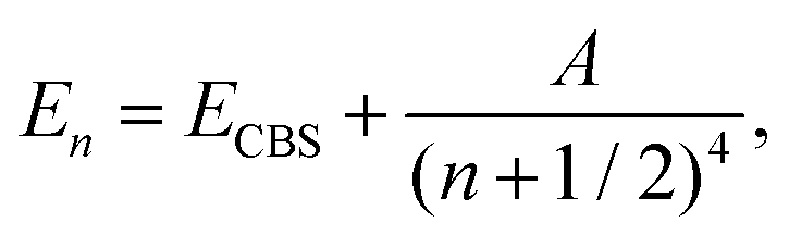
Fig. 1 CASSCF/aVTZ spin-free potential energy curves of the low-lying doublet (black) and quartet (red) states in YO.

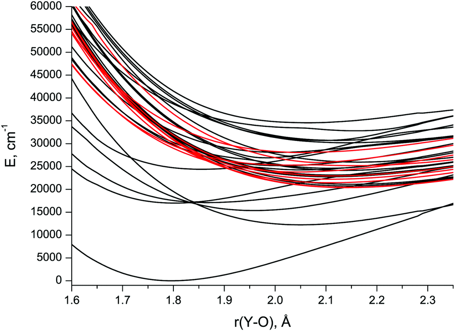
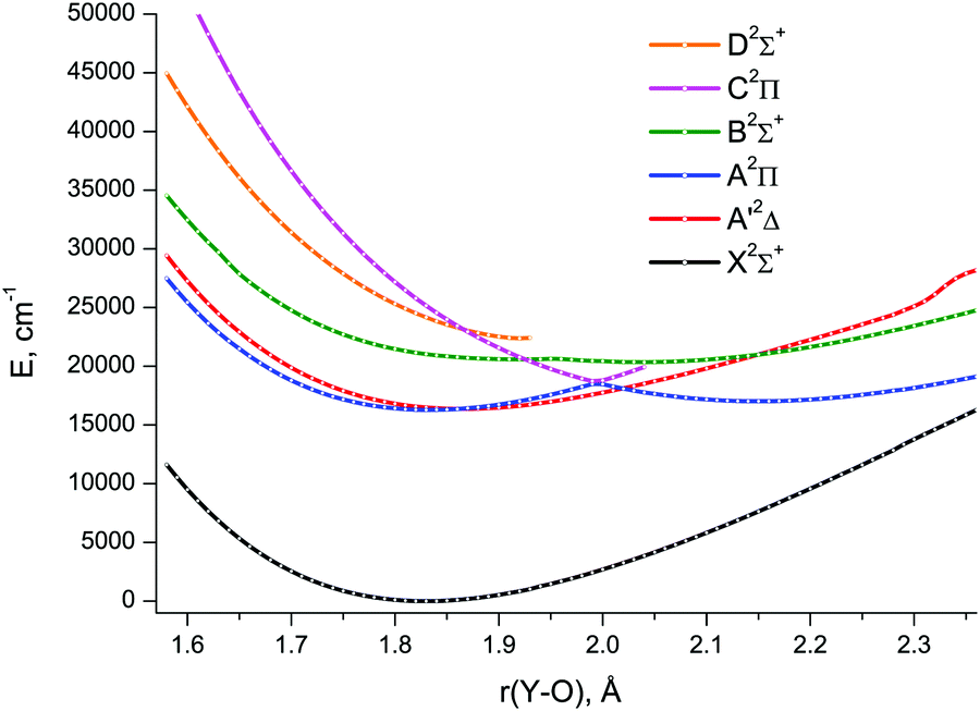
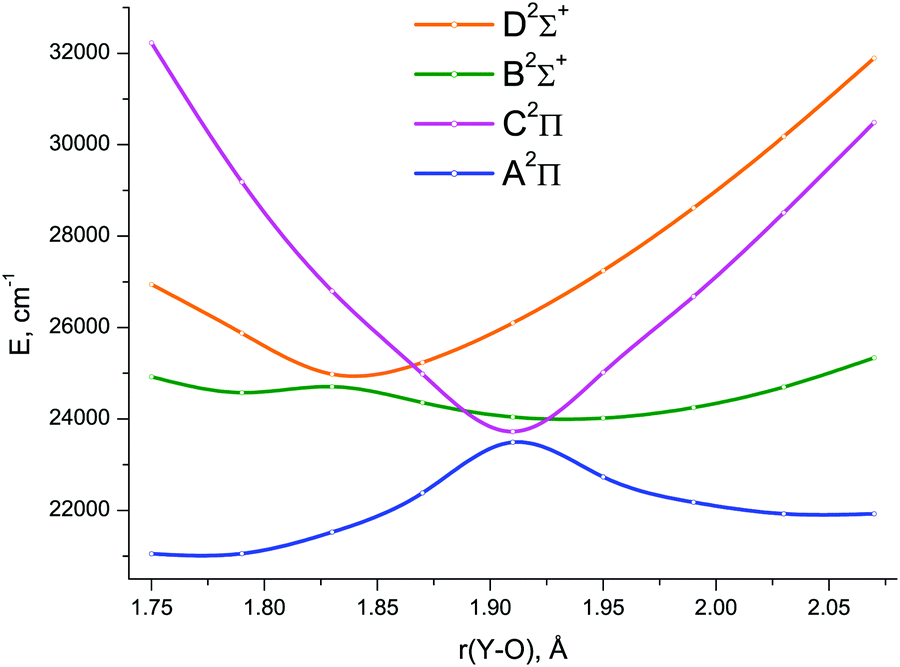
The lowest six doublet MRCI PECs (X²Σ⁺, A′²Δ, A²Π, B²Σ⁺, C²Π, D²Σ⁺) are shown in Fig. 2. For the states X²Σ⁺, A′²Δ, A²Π, and B²Σ⁺, the PECs were obtained in the full bond length range amenable to the underlying CASSCF procedure, 1.58 ≤ r ≤ 2.36 Å, while the C²Π and D²Σ⁺ curves were calculated through r = 2.04 Å and 1.93 Å, respectively. Extending the MRCI curves for the two upper states beyond those distances would require requesting a greater number of states (while exceeding 4 in a single irreducible representation with the chosen active space would make the MRCI computation unfeasible on the hardware used) or selecting the order of the states in the initial internal CI (e.g., 1, 2, 3, 5 rather than 1, 2, 3, 4), leaving some of them out for each MRCI point. This appeared to affect the smoothness of the resulting PECs. Therefore, we refrained from further pursuing the computations with the same number of MRCI roots in the entire bond length range and simply reduced the number of requested states for longer internuclear distances. For all six doublet states, the XMS-CASPT2 PECs could be obtained in the range 1.59 ≤ r ≤ 2.165 Å, Fig. 3; at larger bond lengths the underlying CASSCF procedure failed to converge. As can be seen from Fig. 2 and 3, the A²Π and C²Π curves feature an avoided crossing at bond lengths around 2 Å, as do the B²Σ⁺ and D²Σ⁺ curves in approximately the same region, see Fig. 3. The avoided crossings of both pairs of curves are also seen in the EOM-IP-CCSD calculated PECs, Fig. 4, albeit at shorter distances (1.8–1.9 Å).

Fig. 2 MRCI/aVTZ spin-free potential energy curves of YO.

Fig. 3 XMS-CASPT2/awCVTZ spin-free potential energy curves of YO.

Fig. 4 The avoided crossing regions of the EOM-IP-CCSD/TZ_D spin-free potential energy curves for the A²Π, B²Σ⁺, C²Π, and D²Σ⁺ electronic states of YO.

In order to provide deeper insight into the electronic structure of YO, we analysed the dominant configurations (configuration state functions) in the MRCI wave functions for the lowest electronic states, Table 1, and the leading atomic orbital contributions in the respective molecular orbitals, Table 2.

Table 1 Weights of the leading configurations (configuration state functions) in the low-lying electronic states of YO derived from analyzing the MRCI/aVTZ wave functions at bond lengths of 1.79, 2.04 and 2.19 Å. Contributions of 2% and higher are shown

State	Configurations^a										Weights, %
	10σ	11σ	12σ	13σ	5π+	5π−	6π+	6π−	2δ+	2δ−	1.79 Å	2.04 Å	2.19 Å
a The orbital names π+, π−, δ+, and δ− indicate π(b1), π(b2), δ(a1), and δ(a2) orbitals, respectively. The MO occupancies represented by 2, 0 and + or − denote double, zero, and single occupancies with the total spin raised or lowered by 1/2.
X^2Σ^+	2	2	+	0	2	2	0	0	0	0	79.2	71.4	63.3
	2	+	+	−	2	2	0	0	0	0	2.1	3.1	3.5
	2	+	−	+	2	2	0	0	0	0		2.3	2.8
	2	2	+	0	2	+	0	−	0	0			3.6
	2	2	+	0	+	2	−	0	0	0			3.6
	2	2	+	0	−	2	+	0	0	0			2.2
	2	2	+	0	2	−	0	+	0	0			2.2
A′^2Δ (a1)	2	2	0	0	2	2	0	0	+	0	78.9	67.3	53.1
	2	+	−	0	2	2	0	0	+	0		8.1	21.6
	2	+	0	−	2	2	0	0	+	0	4.8	4.2	4.1
A^2Π (b1)	2	2	0	0	2	2	+	0	0	0	79.9
	2	+	0	−	2	2	+	0	0	0	3.2
	2	2	2	0	+	2	0	0	0	0		82.6	82.3
	2	2	0	0	+	2	2	0	0	0		2.4	2.1
	2	2	0	0	+	2	0	2	0	0		2.1
B^2Σ^+	2	2	0	+	2	2	0	0	0	0	73.5
	2	+	2	0	2	2	0	0	0	0	4.5	80.2	78.9
	2	+	0	2	2	2	0	0	0	0	2.1
	2	+	0	0	2	2	2	0	0	0		2.3	2.0
	2	+	0	0	2	2	0	2	0	0		2.3	2.0
C^2Π (b1)	2	2	2	0	+	2	0	0	0	0	83.2
	2	2	0	0	+	2	2	0	0	0	2.8
	2	2	0	0	+	2	0	2	0	0	2.3
	2	2	0	0	2	2	+	0	0	0		68.7
	2	+	−	0	2	2	+	0	0	0		4.3
	2	+	0	−	2	2	+	0	0	0		3.3
D^2Σ^+	2	+	2	0	2	2	0	0	0	0	79.1
	2	2	0	+	2	2	0	0	0	0	4.0
	2	+	0	0	2	2	2	0	0	0	2.6
	2	+	0	0	2	2	0	2	0	0	2.6

---

Table 2 Analysis of the YO molecular orbitals^a in terms of leading atomic orbital contributions (above 10%) at bond lengths of 1.79, 2.04 and 2.19 Å

MO	1.79 Å	2.04 Å	2.19 Å
a See footnote to Table 1 for designations.
10σ	52% 2s O + 43% 4pσ Y	71% 2s O + 27% 4pσ Y	84% 2s O + 15% 4pσ Y
11σ	63% 2pσ O + 10% 4dσ Y	72% 2pσ O	77% 2pσ O
12σ	86% 5s Y	82% 5s Y + 12% 5pσ Y	81% 5s Y + 13% 5pσ Y
13σ	50% 5pσ Y + 36% 4dσ Y	39% 5pσ Y + 53% 4dσ Y	34% 5pσ Y + 60% 4dσ Y
5π+(−)	94% 2pπ O	95% 2pπ O	96% 2pπ O
6π+(−)	67% 5pπ Y + 32% 4dπ Y	46% 5pπ Y + 52% 4dπ Y	34% 5pπ Y + 63% 4dπ Y
2δ+(−)	100% 4dδ Y	100% 4dδ Y	99% 4dδ Y

---

The analysis indicates that the X²Σ⁺ ground state consists mainly of …10σ²11σ²5π⁴12σ¹ electron configuration. The principal contribution to the singly occupied 12σ MO comes from the yttrium 5s atomic orbital, with an admixture of the 5p AO particularly noticeable at longer internuclear distances. The three lowest active MOs, 10σ, 11σ, and 5π₊₍₋₎, primarily consist of the oxygen 2s and 2p orbitals whose contributions increase with the bond stretching. Therefore, the bonding in the X²Σ⁺ YO ground state can be roughly described as ionic, Y²⁺O²⁻, however, with significant covalent character mainly owing to an appreciable participation of the yttrium 4p_σ AO in the 10σ MO. Upon the Y–O bond stretching, there is a rapid decrease in the 4p contribution (see Table 2) reducing the covalency and resulting in a concomitant increase in the magnitude of the electric dipole moment in the YO ground state (see below).

The first excited state, A′²Δ, mainly consists of …10σ²11σ²5π⁴2δ¹ configuration with the 2δ MO clearly assigned to the Y 4d_δ orbital. At shorter bond lengths this state can be reasonably described by the single electron excitation from the ground state, 5s¹ → 4d_δ¹. Upon bond elongation, the weight of the main configuration gradually decreases, approaching ∼50% at bond lengths of about 2.2 Å, whereas at r > ∼2 Å, a few other large-weight configurations emerge, e.g., the three-open-shell …10σ²11σ^α12σ^β5π⁴2δ^α configuration (with a weight of 22% at 2.19 Å) that corresponds to the Y⁺O⁻ bonding (Y 5s¹4d¹, O 2p⁵).

At bond lengths up to ∼1.85 Å, the principal configurations of the A²Π and B²Σ⁺ excited states, …10σ²11σ²5π⁴6π¹ and …10σ²11σ²5π⁴13σ¹, respectively, include the 6π and 13σ singly occupied MOs mainly composed of the yttrium 5p_π and 5p_σ atomic orbitals, respectively, yet with a significant admixture of the 4d AOs. Therefore, these states can be viewed as arising from 5s → 5p_π and 5s → 5p_σ atomic electron promotions. In the same range of bond length values, the C²Π and D²Σ⁺ upper lying states consist mainly of …10σ²11σ²12σ²5π³ and …10σ²11σ¹12σ²5π⁴ electron configurations, respectively. The YO bonding in the C²Π and D²Σ⁺ states is hence well described by the Y⁺O⁻ scheme consistent with the Y 5s², O 2p⁵ electron configuration.

As the Y–O distance approaches the avoided crossing point from below, the principal configurations of the A²Π and B²Σ⁺ states change to those specified above for the C²Π and D²Σ⁺ states, respectively, while, vice versa, the principal configurations of the C²Π and D²Σ⁺ states turn into those being the main ones for the A²Π and B²Σ⁺ states at shorter bond lengths. This alteration of main configurations describes an oxygen-to-metal charge back-transfer, Y²⁺O²⁻ → Y⁺O⁻, in the A²Π and B²Σ⁺ states of YO upon the Y–O bond stretching through the avoided crossing region of bond lengths.

Specifically, the avoided crossing point, r_ac, chosen to be the point of closest approach of two curves, for the A²Π and C²Π states amounts to 2.046 Å (XMS-CASPT2) and 1.994 Å (MRCI), with the energy gap, ΔE_ac, of 366 cm⁻¹ and 243 cm⁻¹, respectively. For the XMS-CASPT2 B²Σ⁺ and D²Σ⁺ curves, r_ac = 2.064 Å and ΔE_ac = 1484 cm⁻¹. Notably, the principal configuration interchange between the B²Σ⁺ and D²Σ⁺ states occurs at a slightly shorter internuclear distance: ∼1.95 Å (XMS-CASPT2), ∼1.92 Å (MRCI). At the EOM-IP-CCSD level, the avoided crossing characteristics are: r_ac = 1.911 Å, ΔE_ac = 231 cm⁻¹ for A²Π and C²Π curves, and r_ac = 1.832 Å, ΔE_ac = 272 cm⁻¹ for B²Σ⁺ and D²Σ⁺ curves.

The CCSD(T) calculations were carried out for the six lowest doublet states. The reference configurations for each state were as follows:

X²Σ⁺ …10σ²11σ²5π⁴12σ¹

A′²Δ …10σ²11σ²5π⁴2δ¹

A²Π …10σ²11σ²5π⁴6π¹

B²Σ⁺ …10σ²11σ²5π⁴13σ¹

C²Π …10σ²11σ²12σ²5π³

D²Σ⁺ …10σ²11σ¹12σ²5π⁴

The CCSD(T) energies were obtained in the ranges: 1.0 ≤ r ≤ 2.5 Å for X²Σ⁺, A′²Δ and A²Π; 1.0 ≤ r ≤ 2.4 Å for B²Σ⁺; 1.4 ≤ r ≤ 2.4 Å for C²Π; 1.74 ≤ r ≤ 2.35 Å for D²Σ⁺. At longer distances (as well as shorter ones for C²Π and D²Σ⁺), the coupled-cluster calculations failed due to severe CCSD convergence problems. For the X²Σ⁺, A′²Δ, A²Π, and B²Σ⁺ states, the distances shorter than 1.0 Å were not considered because relative energies of excited states already exceed 350 000 cm⁻¹ at this point. The respective CCSD(T)/CBS1 PECs are shown in Fig. 5. Since single reference methods are not suitable for describing avoided crossings, e.g., those between the PECs of the A²Π and C²Π, and B²Σ⁺ and D²Σ⁺ states, the CCSD(T) calculated PECs can be viewed as corresponding to the diabatic presentation of these states. It is clearly seen that the CCSD(T) A²Π and C²Π curves cross each other at 2.031 Å, as do the B²Σ⁺ and D²Σ⁺ ones at 2.013 Å.

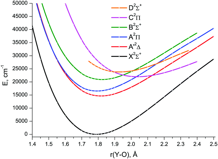Fig. 5 CCSD(T)/CBS1 spin-free potential energy curves of YO.

3.1.2 Spectroscopic constants and excitation energies. Table 3 summarises the optimised bond lengths r_e, harmonic vibrational frequencies ω_e, equilibrium dipole moments μ_e, and adiabatic excitation energies T_e of the low-lying doublet states calculated at the XMS-CASPT2, MRCI and EOM-CCSD levels as well as the results from earlier theoretical studies.^37,53 Our data in the column entitled “C²Π” were obtained from the second minimum in the adiabatic PEC of the A²Π state, i.e., they can be ascribed to the diabatic representation of the A²Π and C²Π states.

Table 3 Theoretical spin-free equilibrium constants of YO in its low-lying doublet states: adiabatic excitation energies, T_e – cm⁻¹, bond lengths, r_e – Å, vibrational frequencies, ω_e – cm⁻¹, and dipole moments μ_e – D. The relevant experimental data are listed in Table 4

		X^2Σ^+	A′^2Δ	A^2Π	B^2Σ^+	C^2Π	D^2Σ^+
a EOM-IP for C^2Π and D^2Σ^+, EOM-EA for the remaining states. b Calculated for each electronic state at the respective CCSD(T)/CBS1 equilibrium bond length. c Calculated at a bond length of 1.7932 Å.
T e	XMS-CASPT2/awCVTZ	0	16 183	16 210	20 521	20 198	24 139
	MRCI/aVTZ	0	16 370	16 287		17 029
	EOM-CCSD/TZD^a	0	16 096	16 817	21 654	21 896	23 995
	MCPF^53	0	15 288	15 728
	MRCI^53	0	15 853	15 655	20 039	20 743
	CASPT2^37	0	15 650	17 340	20 570	21 860	23 800
r e	XMS-CASPT2/awCVTZ	1.822	1.851	1.824	1.858	2.107	1.991
	MRCI/aVTZ	1.830	1.864	1.833		2.149
	EOM-CCSD/TZD^a	1.787	1.811	1.789	1.818	2.049	1.934
	MCPF^53	1.811	1.842	1.813
	MRCI^53	1.814	1.838	1.817	1.842	2.073
	CASPT2^37	1.79	1.82	1.77	1.84	1.97	1.91
ω e	XMS-CASPT2/awCVTZ	796	726	763	696	592	696
	MRCI/aVTZ	777	693	750		542
	EOM-CCSD/TZD^a	881	822	847	804	606	648
	MCPF^53	855	785	832
	MRCI^53	866	801	834	789	638
μ e	MRCI/aVTZ^b	4.410	7.871	4.343	2.971	1.329
	EOM-EA-CCSD/TZD^c	4.905	7.867	4.147	2.164
	MCPF^53	3.976	7.493	3.244

---

The results of our EOM-CCSD calculations indicate that the anionic reference is less suitable for describing YO than the cationic one. In Table 3, more accurate cationic-reference EOM-EA-CCSD spectroscopic constants are listed for all states except for the C²Π and D²Σ⁺ ones which are not accessible via the electron attachment procedure and therefore were described at the EOM-CCSD level only via EOM-IP.

The results given in Table 3 are obviously inferior to those obtained from high-level CCSD(T) calculations including core–valence correlation and extrapolation to the CBS limit. The CCSD(T) results are collected in Table 4 together with the experimental data available to date. The spread in the CCSD(T)/CBS results from different CBS extrapolation schemes serve as a rough estimate of the uncertainty in extrapolation. The good agreement between the CBS estimates and experimentally determined spectroscopic properties of the X²Σ⁺, A′²Δ, A²Π, and B²Σ⁺ electronic states demonstrates the high accuracy in the CCSD(T)/CBS PECs of these states for bond lengths in the vicinity of the PECs minima, and is indicative of the mild MR character of the respective electronic wave functions.

Table 4 CCSD(T) spin-free equilibrium constants of YO in its low-lying electronic states: The dissociation energy D₀ (eV) referring to the ground electronic state X²Σ⁺, the excitation energies T_e (cm⁻¹) of the A′²Δ, A²Π, B²Σ⁺, C²Π D²Σ⁺, and a⁴Π states, bond length r_e (Å), spectroscopic constants ω_e (cm⁻¹), ω_ex_e (cm⁻¹) and α_e (cm⁻¹), and dipole moment μ_e (D)

		X^2Σ^+	A′^2Δ	A^2Π	B^2Σ^+	C^2Π	D^2Σ^+	a^4Π
D 0, Te	awCVTZ	7.060						28 924
	awCVQZ	7.207	14 809	16 555	20 893	21 423	23 261	29 296
	awCV5Z	7.260	14 712	16 538	20 898	21 700	23 528	29 465
	CBS1	7.298	14 633	16 526	20 901	21 925	23 745	29 603
	CBS2	7.298	14 629	16 525	20 897	21 917	23 741	29 592
	CBS3	7.289						29 564
	Expt	7.290(87)^52	14 701^38	16 530^35	20 793^35		23 972^37
r e	awCVTZ	1.7978						2.0902
	awCVQZ	1.7927	1.8201	1.7971	1.8268	2.0408	1.9345	2.0841
	awCV5Z	1.7905	1.8177	1.7950	1.8244	2.0384	1.9323	2.0817
	CBS1	1.7887	1.8157	1.7932	1.8225	2.0365	1.9306	2.0797
	CBS2	1.7890	1.8160	1.7935	1.8228	2.0368	1.9308	2.0799
	CBS3	1.7892						2.0802
	Expt	1.7882^11	1.817^39	1.7931^13	1.8252^35
ω e	awCVTZ	855.2						546.0
	awCVQZ	861.4	794.0	822.5	780.6	601.8	661.2	550.6
	awCV5Z	864.2	797.1	825.1	783.2	603.3	662.3	552.1
	CBS1	866.5	799.7	827.1	785.3	604.6	663.1	553.3
	CBS2	866.2	799.4	826.8	785.1	604.6	663.1	553.3
	CBS3	865.8						552.9
	Expt	861.5^11	794^49	820^35	765^21
					759^35
ω e x e	awCVTZ	2.79						2.52
	awCVQZ	2.78	3.06	3.17	2.94	2.58	2.60	2.53
	awCV5Z	2.79	3.05	3.18	2.98	2.57	2.60	2.57
	CBS1	2.79	3.04	3.19	3.01	2.57	2.61	2.60
	CBS2	2.79	3.03	3.18	3.01	2.57	2.61	2.60
	CBS3	2.79						2.59
	Expt	2.84^11	3.23^38	3.15^11	3.97^35
				3.35^13
α e × 10^3	awCVTZ	1.70						1.83
	awCVQZ	1.68	1.85	1.90	1.86	1.79	1.85	1.83
	awCV5Z	1.68	1.85	1.91	1.87	1.80	1.86	1.83
	CBS1	1.68	1.85	1.91	1.87	1.80	1.87	1.83
	CBS2	1.68	1.84	1.91	1.87	1.80	1.87	1.83
	CBS3	1.68						1.83
	Expt	1.73^11	1.7^38	2.01^13	2.49^35
μ e	awCVTZ	4.615	7.595	3.711	1.749	2.059	1.256	3.605
	awCVQZ	4.614	7.620	3.724	1.764	2.082	1.275	3.615
	awCV5Z	4.611	7.626	3.728	1.770	2.090	1.281	3.618
	CBS1	4.609	7.630	3.730	1.775	2.097	1.287	3.621
	CBS2	4.609	7.630	3.731	1.777	2.097	1.287	3.621
	CBS3	4.609	7.629	3.729	1.774	2.095	1.285	3.620
	Expt	4.45(7)^27		3.68(2)^27
		4.524(7)^45

---

An insight into the reliability of the CCSD(T) PECs over the entire bond length range explored, and for all electronic states considered, including those not yet characterised experimentally, can be provided by using the MR diagnostic criteria commonly employed to identify the suitability of single reference wavefunction-based methods: T₁,⁹⁵ the Frobenius norm of the coupled cluster amplitude vector related to single excitations, and D₁,⁹⁶ the matrix norm of the coupled cluster amplitude vector arising from coupled cluster calculations. The utility of different MR diagnostics has been examined in earlier studies^97,98 on various 3d and 4d TM species. The following criteria have been proposed⁹⁸ as a gauge for the latter to predict the possible need to employ multireference wavefunction-based methods while describing energetic and spectroscopic molecular properties: T₁ ≥ 0.045, D₁ ≥ 0.120, %TAE[(T)] ≥ 10%. The symbol %TAE[(T)] denotes here the percent total atomization energy corresponding to a relationship between energies determined with CCSD and CCSD(T) calculations.^99,100 Obviously, the %TAE[(T)] diagnostic is applicable for judging the SR/MR character of the electronic ground state only. For the YO molecule, the CCSD/awCV5Z calculated %TAE[(T)] of 5.6% is well below the proposed MR threshold. This fact provides further evidence for single reference character of the X²Σ⁺ wavefunction in the near-equilibrium region of Y–O bond lengths.

The CCSD/awCV5Z T₁ plots vs. Y–O bond length are shown in Fig. 6. The similar D₁ plots are illustrated in Fig. S1 of the ESI.† At shorter bond lengths, the diagnostics amount to 0.02–0.03 (T₁) and 0.05–0.12 (D₁), remaining below the MR thresholds down to 1.4 Å for most states. Upon bond stretch, T₁ and D₁ rapidly increase, typically exceeding the MR threshold at 2.1–2.2 Å. The behaviour of these diagnostics for the C²Π state is a notable exception: the numerical values of both T₁ and D₁ remain well below the MR threshold throughout the bond length range studied. The D²Σ⁺ state is also noteworthy: its T₁ and D₁ diagnostics are indicative of the CCSD D²Σ⁺ wave function retaining its SR character in much narrower range of bond lengths compared to the other doublet states under study.

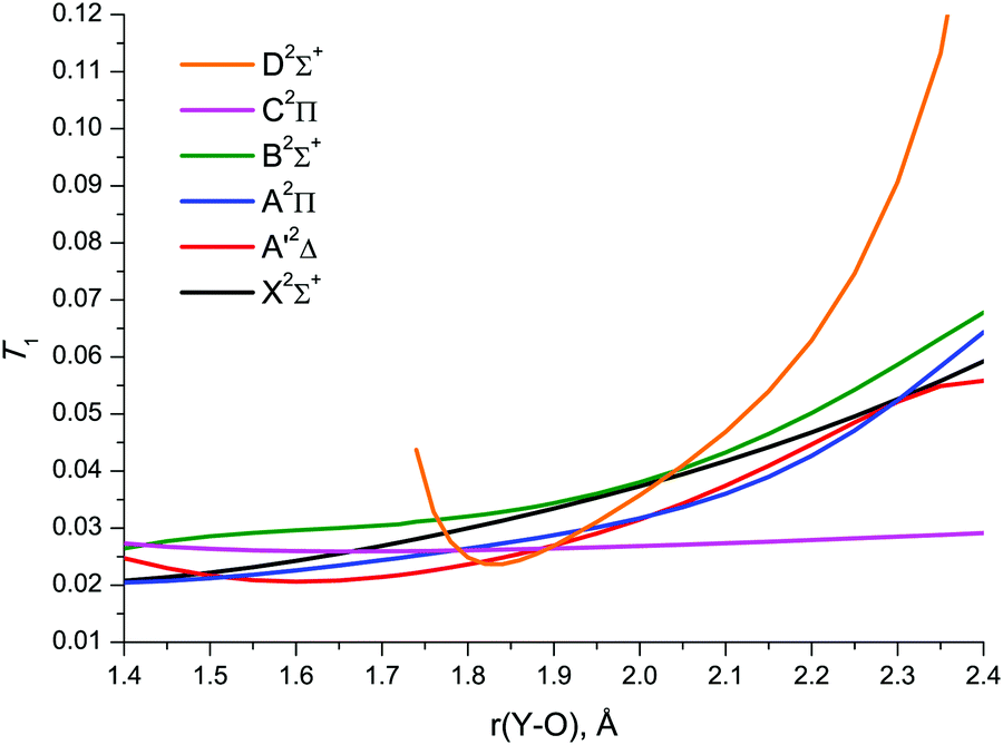Fig. 6 The CCSD/awCV5Z calculated T₁ diagnostics of YO.

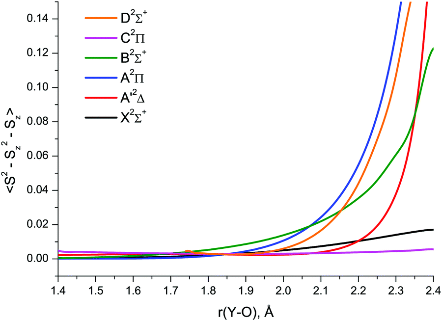
The relative importance of SR/MR character of YO can also be guessed with the use of spin contamination appearing in RHF-UCCSD calculations as a result of unrestricted spin at the CCSD level. According to Jiang et al.,⁹⁷ spin contamination with 〈S² − S_z² − S_z〉 greater than 0.1 in an RHF-UCCSD wave function can be viewed as a strong indication of nondynamical correlation in an open-shell system. Plotting spin contamination vs. bond length, Fig. 7, clearly indicates the severe admixture of higher spin states in the CCSD A′²Δ, A²Π, B²Σ⁺ and D²Σ⁺ wave functions at bond lengths beyond 2.2–2.3 Å. Greater extent of spin contamination at longer internuclear distances can obviously be associated with larger values of T₁ and D₁ (Fig. 6 and Fig. S1 of the ESI†) exceeding the established MR thresholds.

Fig. 7 RHF-UCCSD/awCV5Z wave function spin contamination in the low-lying doublet electronic states of YO.

It is instructive to compare the MR diagnostics discussed above with the weights of the principal configurations, C₀², in the MRCI wavefunctions of YO (see Table 1). At shorter bond lengths, the C₀² values amount to ∼0.73 for the B²Σ⁺ state and 0.79–0.83 for the remaining doublet electronic states under study. These values are smaller than the threshold, C₀² ≥ 0.90, proposed in ref. 97 and 98 to recognise the wave function strongly dominated by a single configuration. It should, however, be noted that this criterion was established by analyzing the CASSCF wavefunctions, whereas the C₀² of the entire MRCI wavefunction differs from that of the CASSCF reference function due to the contributions of external configurations, which make C₀² a smaller number.

Upon the YO bond stretch, there is a gradual decrease in the weights of the configurations serving as a reference for the coupled cluster treatment of the X²Σ⁺, A′²Δ, and A²Π states. This indicates greater multireference character of the respective wave functions at longer bond distances, as do the CC-based MR diagnostics. The reference configuration for the C²Π state has approximately the same weight, C₀² ≅ 0.83, in the MRCI wavefunctions of YO throughout the bond length range explored, behaving just like the respective CC-based MR diagnostics. These examples of the CCSD-MRCI correlations imply that the CC-based MR diagnostics can be capable of providing qualitative data about the relative accuracy in the single-reference coupled cluster calculation results not only for near-equilibrium regions of electronic ground states, but also for excited states in a wider range of molecular geometries.

In general, the present analysis indicates essentially single reference character of the YO low-lying doublet states over most part of bond length range explored in our work and hence high accuracy in the respective domains of the CCSD(T) PECs. It may also be indicative of accuracy degradation at larger bond lengths, implying the need for additional adjustments of the CCSD(T) PECs. Nevertheless, the bond length range associated with high-energy sections of PECs is expected to have a limited impact on the simulated spectra.

3.1.3 Quartet states. We studied five low-lying quartet electronic states of YO at the CASSCF, CASPT2, CASPT3, and MRCI levels of theory using the aVTZ basis set. The results are shown in Table 5 together with the earlier theoretical findings.⁵³ The lowest quartet, a⁴Π, was also studied at the CCSD(T) level (Table 4). At larger internuclear distances, e.g., at r = 2.19 Å, all the quartets feature similar orbital character corresponding to the Y 5s¹4d¹, O 2p⁵ electron configuration consistent with the Y⁺O⁻ bonding (see Table 6).

Table 5 Theoretical spin-free equilibrium constants of YO in its low-lying quartet states: adiabatic excitation energy T_e – cm⁻¹, bond length r_e – Å, vibrational frequency ω_e – cm⁻¹. The aVTZ basis set has been used throughout

		^4Π	^4Φ	^4Σ^+	^4Δ	^4Σ^−
a The energies of the ^4Φ, ^4Σ^+, ^4Δ and ^4Σ^− states are given here with respect to the ^4Π state which is the lowest-lying quartet state of YO. b In ref. 53, the symmetry of the lowest quartet state of YO was reported to be ^4Φ rather than ^4Π. c In ref. 53, the adiabatic excitation energy of the lowest quartet state was obtained from the MCPF calculations, and the relative energies of various quartet states were determined at the CASSCF level.
T e	CASSCF	20 460	68	1062	1825	2542
	CASPT2	24 140	56	1432	2158	2785
	CASPT3	23 772	53	1450	2175	2788
	MRCI	25 046	55	1394	2128	2748
	MRCI + Q	26 274	59	1357	2089	2699
	CASSCF^53	26 975^b^,^c	52	1933	2664	3359
r e	CASSCF	2.141	2.143	2.110	2.110	2.114
	CASPT2	2.197	2.198	2.192	2.191	2.196
	CASPT3	2.210	2.211	2.207	2.208	2.214
	MRCI	2.213	2.214	2.209	2.209	2.214
	MRCI + Q	2.218	2.219	2.218	2.218	2.222
	CASSCF^53	2.121^b	2.122	2.108	2.109	2.114
	MCPF^53	2.126^b
ω e	CASSCF	517	516	522	521	519
	CASPT2	515	515	517	494	477
	CASPT3	519	518	524	494	474
	MRCI	507	507	501	495	492
	MRCI + Q	506	506	501	496	493
	CASSCF^53	543	543	524	522	520
	MCPF^53	526^b

---

Table 6 Main configurations in the low-lying quartet electronic states of YO derived from analyzing the MRCI/aVTZ wave function at a bond length of 2.19 Å. Weight of each configuration is ∼45%

State	Configurations^a
	10σ	11σ	12σ	13σ	5π+	5π−	6π+	6π−	2δ+	2δ−
a See footnote to Table 1 for designations.
^4Π(b1)	2	2	+	0	+	2	0	0	+	0
	2	2	+	0	2	+	0	0	0	+
^4Φ(b1)	2	2	+	0	+	2	0	0	+	0
	2	2	+	0	2	+	0	0	0	+
^4Σ^+	2	2	+	0	+	2	+	0	0	0
	2	2	+	0	2	+	0	+	0	0
^4Δ(a1)	2	2	+	0	+	2	+	0	0	0
	2	2	+	0	2	+	0	+	0	0
^4Σ^−	2	2	+	0	+	2	0	+	0	0
	2	2	+	0	2	+	+	0	0	0

---

The results for the YO quartet states obtained in our work agree with those of Langhoff and Bauschlicher,⁵³Table 5, except for the symmetry of the lowest quartet state that was reported⁵³ to be ⁴Φ rather than ⁴Π.

The single-reference CCSD(T) method is expected to yield quite accurate results for the a⁴Π state of YO since its MR diagnostics, C₀² = 0.90, T₁ = 0.024, and D₁ = 0.078, indicate essentially SR character of the a⁴Π wave function in the vicinity of the a⁴Π PEC minimum, 2.00–2.25 Å. The very large CCSD(T)/CBS excitation energy of the a⁴Π state, 29 600 cm⁻¹, suggests that the quartet states in YO are too high in energy to significantly affect the spectroscopy of its low-lying doublet states.

3.1.4 SO coupling. Spin–orbit coupling effects were studied in a perturbative fashion at the MRCI level and more rigorously at the 4c-EOM-CCSD level of theory including spin from the outset. The 4c-EOM-CCSD calculated spin–orbit coupling effects on the spectroscopic constants of YO are shown in Table 7. The theoretical spin–orbit coupling constants, SOCCs (A_SO), can be compared with the relevant experimental numbers for the A′²Δ and A²Π electronic states of YO reported previously.^11,13,38 The A_SO(A′²Δ) SOCCs of 336 cm⁻¹ and 313 cm⁻¹ obtained at the MRCI SI-SO and 4c-EOM-CCSD levels, respectively, agree well with each other and with the experimental number of 339 cm⁻¹ determined by Chalek and Gole.³⁸ The calculation results for A_SO(A²Π), 346 cm⁻¹ (MRCI SI-SO) and 438 cm⁻¹ (4c-EOM-CCSD), are also in reasonable agreement with the respective experimental value of 428 cm⁻¹.^11,13 As the Y–O distance reaches the avoided crossing point between A²Π and C²Π, the A_SO(C²Π) and A_SO(A²Π) values change their sign: the A²Π_3/2 spin component of the A²Π state becomes lower in energy than its A²Π_1/2 counterpart, and vice versa for the spin-coupled components of the C²Π state (see Fig. 8). There is also a change in the absolute values of A_SO(A²Π) and A_SO(C²Π): at r < r_ac, |A_SO(A²Π)| is much lower in magnitude than |A_SO(C²Π)| and vice versa at r > r_ac. However, the numerical values of A_SO(A²Π) at r > r_ac determined with the MRCI SI-SO and 4c-EOM-CCSD methods, e.g., −45 cm⁻¹ and −186 cm⁻¹, respectively, at a bond length of 2.04 Å, are in less satisfactory agreement with each other than those at r < r_ac.

Table 7 4c-EOM-CCSD/TZ_D molecular properties of YO in its low-lying spin-coupled electronic states (EOM-IP for C²Π and EOM-EA for the remaining states): bond length r_e – Å, vibrational frequency ω_e, adiabatic excitation energy T_e – cm⁻¹. The respective spin–orbit effects, Δ_SO, are provided as well

	r e	ΔSOre	ω e	ΔSOωe	T e	ΔSOTe
X^2Σ^+1/2	1.7866	0.0000	880.9	0.0	0	0
A′^2Δ3/2	1.8109	+0.0003	821.5	−0.5	15 937	−159
A′^2Δ5/2	1.8102	−0.0004	822.6	+0.6	16 254	+157
A^2Π1/2	1.7892	+0.0005	846.9	−0.5	16 591	−226
A^2Π3/2	1.7884	−0.0003	847.8	+0.4	17 028	+212
B^2Σ^+1/2	1.8181	−0.0003	804.5	+0.6	21 671	+17
C^2Π3/2	2.0488	−0.0004	605.7	+0.1	21 808	−88
C^2Π1/2	2.0495	+0.0003	605.6	−0.0	21 994	+98

---

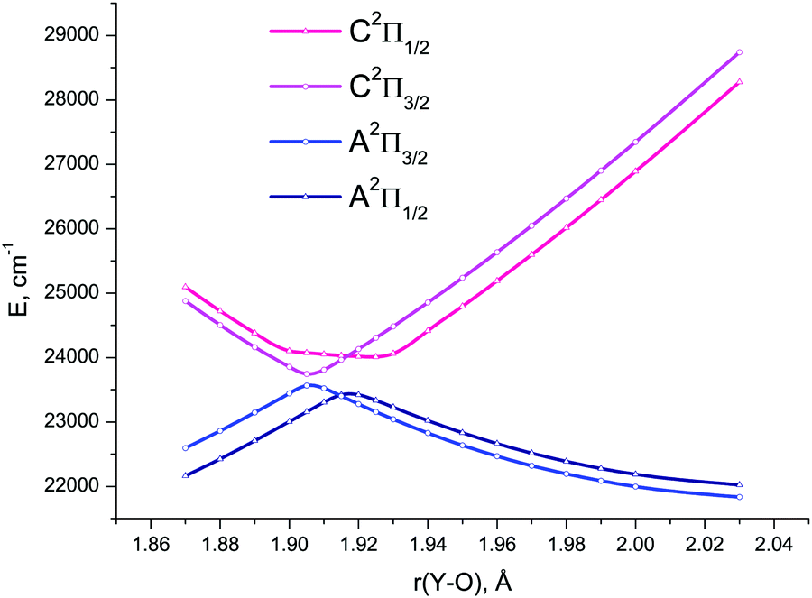Fig. 8 4c-EOM-IP-CCSD/TZ_D potential energy curves for the spin-coupled components of the A²Π and C²Π electronic states of YO in the avoided crossing region of bond length values.

The SOC matrix elements between various doublet states of YO, which also accurately account for the corresponding phases, are shown in Fig. 9 as a function of r(Y–O). The relative phases of the couplings are important when used for solving the nuclear motion problem as part of the coupled Schrödinger equation, see, for example, discussion by Patrascu et al.⁹² The full details of the ab initio coupling curves including the magnetic quantum numbers are provided as part of the ESI.†

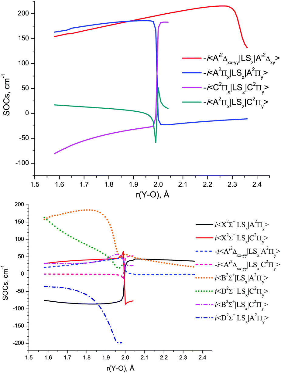Fig. 9 The MRCI/aVTZ SI-SO calculated 〈i|LS_z|j〉 (above) and 〈i|LS_x|j〉 (below) spin–orbit matrix elements of YO.

3.1.5 Dipole moment, transition dipole moment, and electronic angular momentum curves of YO. The CCSD(T)/CBS dipole moment of 4.61 D for the X²Σ⁺ state of YO (Table 4) is in agreement with the respective values obtained experimentally by Steimle and Shirley²⁷ in a molecular beam-optical Stark study, 4.45(7) D, and by Suenram et al.⁴⁵ from the more precise microwave measurement, 4.524(7) D. For the spin–orbit components Ω = 1/2 and Ω = 3/2 of the A²Π state, the dipole moment values, μ_e(A²Π_1/2) = 4.185 D and μ_e(A²Π_3/2) = 4.125 D, were obtained at the 4c-EOM-EA-CCSD/TZ_D level of theory at the respective CCSD(T)/CBS equilibrium bond lengths of 1.7937 Å and 1.7929 Å, estimated by applying the 4c-EOM-EA-CCSD Δ_SOr_e spin–orbit corrections (from Table 7) to the spin-free CCSD(T)/CBS1 bond length, r_e = 1.7932 Å. The 4c-EOM-EA-CCSD dipole moments are overestimated by 0.4–0.5 D compared to the spin-free CCSD(T)/CBS μ_e(A²Π) value of 3.73 D, the latter being in good agreement with the μ_e(A²Π_3/2) = 3.68(2) D measured by Steimle and Shirley.²⁷ However, the experimental work²⁷ reports the dipole moment μ_e(A²Π_1/2), 3.22(8) D, to be lower than μ_e(A²Π_3/2). This result is not supported by our ab initio calculations. Steimle and Shirley²⁷ compared the dipole moments in the A²Π spin–orbit components of YO to those of the valence-isoelectronic molecule ScO,¹⁰¹ where μ_e(A²Π_1/2) > μ_e(A²Π_3/2), and proposed an explanation of the different order in YO. According to Steimle and Shirley,²⁷ the reason for μ(A²Π_3/2) being larger than μ(A²Π_1/2) in YO in contrast to ScO is the smaller energy gap of the A²Π and A′²Δ states, which results in mixing between the Ω = 3/2 spin–orbit components of these states. This idea is, however, based on low-level ab initio computations by Langhoff and Bauschlicher,⁵³ which predicted the A′²Δ state in YO to lie 200 cm⁻¹ higher than A²Π, whereas for ScO the analogous calculations¹⁰² yielded a difference of about 1900 cm⁻¹, with A′²Δ being lower in energy. In fact, the A′²Δ state lies around 1800 cm⁻¹ lower than A²Π in YO and 1500 cm⁻¹ lower in ScO, as evidenced by experimental works of Chalek and Gole,^38,49i.e., the A²Π–A′²Δ energy gap in YO exceeds that in ScO. Also, at high levels of theory including SO coupling, the PECs for the Ω = 3/2 components of A²Π and A′²Δ lie quite far apart (see the excitation energies in Table 7), and their mixing is almost negligible. Furthermore, it is worth noting that for another analogous molecule, LaO, the experimental data¹⁰³ also indicate that μ_e(A²Π_1/2) > μ_e(A²Π_3/2).

To shed more light on the alleged different order of the dipole moment values for the spin–orbit components of the A²Π state in YO compared to ScO and LaO, we performed additional 4c-EOM-EA-CCSD/TZ_D computations for the two latter molecules at the experimental equilibrium bond lengths^104,105 of 1.6826 Å (ScO) and 1.8400 Å (LaO). These resulted in the following values: μ(A²Π_1/2) = 4.543 D, μ(A²Π_3/2) = 4.532 D (ScO), μ(A²Π_1/2) = 3.011 D, μ(A²Π_3/2) = 2.907 D (LaO), i.e., the ab initio predicted difference between the two spin–orbit components monotonically increases on passing in the series ScO → YO → LaO: 0.01 → 0.04 → 0.10 D, respectively. The experimental counterparts^101,103 are: μ(A²Π_1/2) = 4.43(2) D, μ(A²Π_3/2) = 4.06(3) D (ScO), μ(A²Π_1/2) = 2.44(2) D, μ(A²Π_3/2) = 1.88(6) D (LaO). Since the 4c-EOM-EA-CCSD dipole moments are expected to be overestimated by at least 0.5 D, one can consider the theoretical results to be in reasonable agreement with experiment. In light of our results, the experimental dipole moments²⁷ for the two Ω components of the A²Π state of YO need to be revisited.

The MCPF dipole moments obtained by Langhoff and Bauschlicher,⁵³ 3.976 D (X²Σ⁺), 7.493 D (A′²Δ) and 3.244 D (A²Π), are systematically smaller than our CCSD(T) (Table 4), MRCI, and EOM-EA-CCSD (Table 3) results.

The MRCI DMCs and TDMCs of YO are shown in Fig. 10. The EAMCs are shown in Fig. S2 of the ESI.† All these curves as well as the SOC ones (Fig. 9) exhibit irregular behaviour at bond lengths around r ∼ 2 Å due to strong changes in the A²Π, B²Σ⁺, C²Π and D²Σ⁺ wave functions over the avoided crossing region.

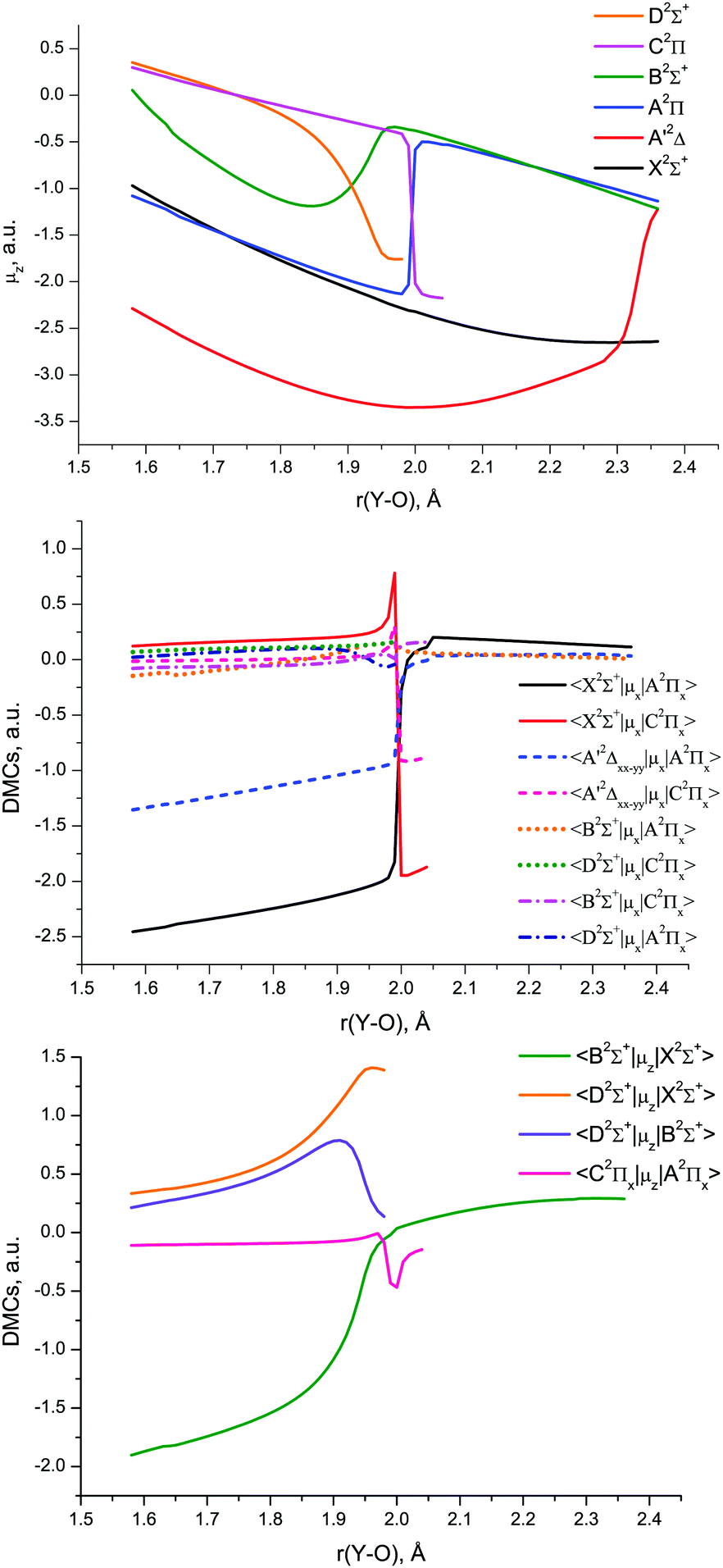Fig. 10 MRCI/aVTZ electric dipole moment curves of YO: diagonal (above), non-diagonal μ_x (middle) and non-diagonal μ_z (below).

3.2 Results of Duo calculations

For Duo calculations, we selected the following set of curves representing our highest level of theory: the CCSD(T)/CBS PECs shown in Fig. 5 and MRCI SOCs, (T)DMCs, and EAMCs shown in Fig. 9 and 10, as well as Fig. S2 of the ESI.† Due to limitations of single reference CCSD(T), the CCSD(T) curves for the A²Π, C²Π and B²Σ⁺, D²Σ⁺ states do not exhibit avoided crossings and hence are not consistent with the MRCI property curves. To alleviate this deficiency, these four PECs were transformed by simply switching the corresponding energy points between A and C (²Π states) as well as those between B and D (²Σ⁺ states) at r > r_ac. We have decided to apply this rather simplistic procedure because it has marginal effect on the overall accuracy of our model and is sufficient for the goal of this pure ab initio study, not aiming at spectroscopic accuracy. A proper diabatic representation of the YO electronic states will be, however, important when refining the ab initio curves by fitting to experiment,⁹³ which is a goal of future work. In this study we work directly with the ab initio data in the grid representation without representing ab initio curves analytically. We do not perform any diabatizations here, which is often useful for representing the variation of the data with respect to the bond length in an intuitive and more compact form. One of the artifacts of this choice to use the ab initio curves directly is that the crossing points of the MRCI PECs hence the points of drastic change in the MRCI property curves differ by a few hundredths of Å from the crossing points of the CCSD(T)/CBS PECs. Again, this has small impact on the overall agreement of the current model with the experiment. However, a more accurate study will require a more consistent treatment of the crossing points. Our preferred choice would be to use the CCSD(T)/CBS values of the corresponding crossing points.

The Duo rovibronic wavefunctions of YO in conjunction with the ab initio TDMCs were then used to produce Einstein A coefficients for all rovibronic transitions between states considered in this work covering the wavenumber range from 0 to 40 000 cm⁻¹ and J ≤ 180.5. These Einstein A coefficients and the corresponding energies from the lower and upper states involved in each transition were organised as a line list using the ExoMol format.¹⁰⁶ This format uses a two file structure with the energies included into the States file (.states) and Einstein coefficients appearing in the Transitions file (.trans). This ab initio line list is available from http://www.exomol.com. The ExoMol format has the advantage of being compact and compatible with our intensity simulation program ExoCross¹⁰⁷ (see below).

3.2.1 Vibronic energies. In Table 8 we compare our computed vibrational excitations at J = 0.5 and J = 1.5 (as proxy for vibrational band centres) of ⁸⁹Y¹⁶O with the experimentally derived values. Based on this comparison, as an ad hoc improvement we applied the following shifts to PECs of the excited states: +9.509 cm⁻¹ (A²Π), +81.096 cm⁻¹ (A′²Δ), −134.301 cm⁻¹ (B²Σ⁺), and +358.626 cm⁻¹ (D²Σ⁺). These shifts are small compared to the observed minus calculated differences often encountered in calculations of electronic term values for transition metal oxides.⁶⁰ We also scaled the SOC of A²Π by 1.14 in order to increase the SO splitting of v = 0 by about 33 cm⁻¹. Even though we are not targeting fully quantitative accuracy in this work, without such empirical shifts it would be difficult to reproduce band heads even qualitatively.

Table 8 Comparison of our ab initio and experimentally derived term values of ⁸⁹Y¹⁶O in cm⁻¹. The ab initio PECs were shifted by +9.509 cm⁻¹ (A²Π), +81.096 cm⁻¹ (A′²Δ), −134.301 cm⁻¹ (B²Σ⁺) and +358.626 cm⁻¹ (D²Σ⁺). The SOC of A²Π was scaled by 1.1376. The ‘Obs’ values of A, A′, B and D were derived using spectroscopic constants from the corresponding works with the help of the PGOPHER program.¹⁰⁸ The X state ‘Obs.’ values are represented by the corresponding band centers (limit J = 0)

	υ	J	Ω	Duo	Obs.
a Band centres.
					ref. 109	ref. 13
X^a	0	0		0	0	0
	1	0		860.879	855.2	855.7463(52)
	2	0		1716.156	1704.4	1705.8339(90)
	3	0		2565.836	2547.9	2550.2684(65)
	4	0		3409.931	3385.4	3389.0242(90)
	5	0		4248.450	4217.1	4222.085(11)
	6	0		5081.364		5049.454(13)
					ref. 13
A	0	0.5	0.5	16295.492	16295.453
	0	1.5	1.5	16724.499	16724.541
	1	1.5	1.5	17117.400	17109.845
	1	1.5	1.5	17545.141	17538.459
	2	1.5	1.5	17931.536	17916.880
	2	1.5	1.5	18358.848	18345.768
	3	1.5	1.5	18740.505	18716.674
	3	1.5	1.5	19169.245	19146.593
	4	1.5	1.5	19547.495	19510.064
	4	1.5	1.5	19964.360	19940.488
	5	1.5	1.5	20350.928	20296.636
	5	1.5	1.5	20732.561	20727.595
					ref. 39
A′	0	2.5	1.5	14500.074	14502.010
					ref. 21	ref. 35
B	0	0.5	0.5	20741.630	20741.688	20741.6877
	1	0.5	0.5	21516.945		21492.4773
	2	0.5	0.5	22294.044
	3	0.5	0.5	23102.252		22941.71
	4	0.5	0.5	23850.742		23615.3
					ref. 37
D	0	0.5	0.5	23969.916	23969.940
	1	0.5	0.5	24659.745	24723.766

---

To allow for a direct comparison with the observed spectra of ⁸⁹Y¹⁶O, we generated a line list covering rotational excitations up to J = 190 and the energy/wavenumber range up to 40 000 cm⁻¹, with a lower state energy cutoff of 16 000 cm⁻¹.

3.3 Partition function

The partition function of ⁸⁹Y¹⁶O computed using our ab initio line list is shown in Fig. 11, which is compared to that recently reported by Barklem and Collet.¹¹⁰ Since ⁸⁹Y has a nuclear spin degeneracy of two, we have multiplied Barklem and Collet's partition function by a factor of two to compensate for the different conventions used; we follow HITRAN¹¹¹ and include the full nuclear spin in our partition functions. The partition function of YO was also reported by Vardya,¹¹² which is shown in Fig. 11. All three partition functions are almost identical for their ranges of validity.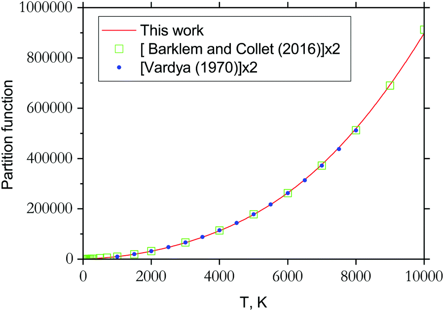

Fig. 11 Partition functions of YO: solid line is from this work computed using the energies of the six lowest electronic states; filled circles represent the partition function values by Vardya¹¹² generated using spectroscopic constants of 3 lowest electronic states X, A and B (multiplied by a factor of 2 to account for the nuclear statistics); open squares represent values by Barklem and Collet¹¹⁰ (times the factor 2).

3.4 Spectral comparisons

Using the ab initio⁸⁹Y¹⁶O line list, spectral simulations were performed with our code ExoCross.¹⁰⁷ ExoCross is an open source Fortran 2003 code with the primary use to produce spectra of molecules at different temperatures and pressures in the form of cross sections using molecular line lists as input. Here we use the YO line list generated with Duo in the ExoMol format, the description of which can be found, e.g., in Yurchenko et al.¹⁰⁷ or Tennyson et al.¹⁰⁶ ExoCross can be accessed viahttp://exomol.com/software/ or directly at https://github.com/exomol. Amongst other features, ExoCross can generate spectra for non-local thermal equilibrium conditions characterised with different vibrational and rotational temperatures, lifetimes, Landé g-factors, partition and cooling functions.

An overview of the YO absorption spectra in the form of cross sections at the temperature T = 2000 K is illustrated in Fig. 12. Here, a Gaussian line profile with a half-width-at-half-maximum (HWHM) of 5 cm⁻¹ was used. This figure shows contributions from each electronic band originating from the ground electronic state. The strongest bands are A²Π–X²Σ⁺ and B²Σ⁺–X²Σ⁺. The visible A–X band is known to be important for the spectroscopy of cool stars. The C state is of the same symmetry as A, however, the corresponding band C–X is much weaker due to the small Franck–Condon effects. The A′²Δ–X²Σ⁺ band is forbidden and barely seen in Fig. 12, however, it is strong enough to be experimentally known.³⁹

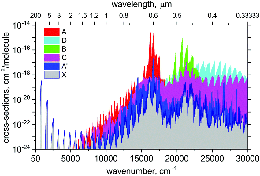Fig. 12 An overview of a theoretical absorption spectrum of YO at T = 2000 K for different electronic bands, designated by their upper state. The spectrum was computed using our ab initio line list for YO assuming a Gaussian profile with a half-width-at-half-maximum (HWHM) of 5 cm⁻¹.

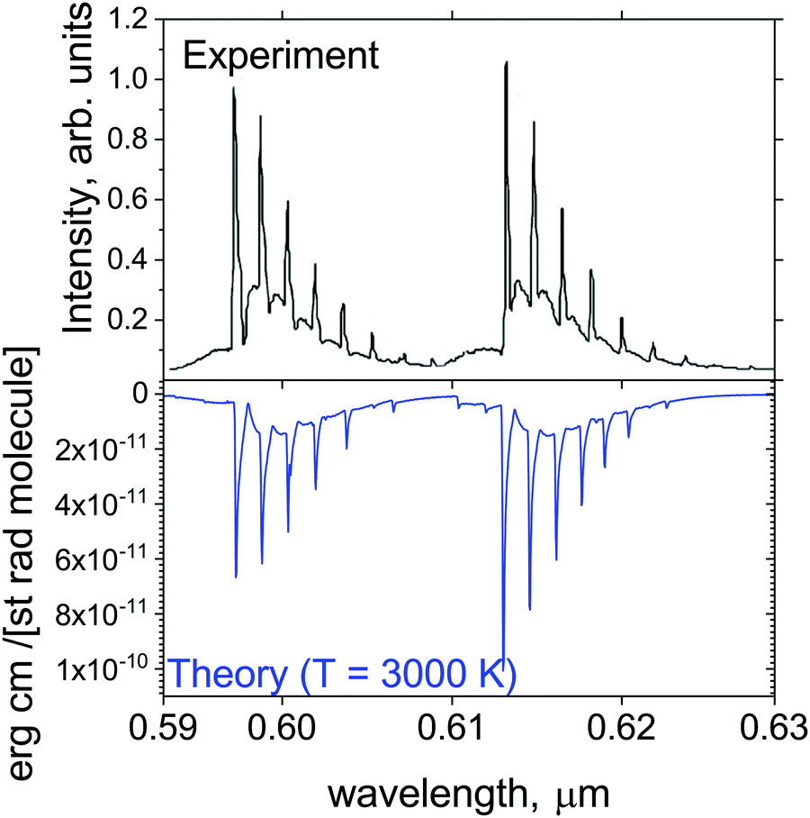
Fig. 13 shows a simulated emission spectrum of the strongest orange system YO (A²Π–X²Σ⁺, (0,0)), which is compared to the experiment of Badie and Granier³¹ (from the plume emission close to the liquid Y₂O₃ surface). It is remarkable that even pure ab initio calculations (after modest adjustment of the corresponding T_e value by +9.509 cm⁻¹) provide very close reproduction of experiment. It shows that our line list at the current, ab initio quality should be useful for modelling spectroscopy of exoplanets and cool stars in the visible region.

Fig. 13 Comparison of the computed A²Π–X²Σ⁺ orange band with the observations of Badie and Granier.³¹ Our simulations assume T = 3000 K and Gaussian line profile of HWHM = 1 cm⁻¹.

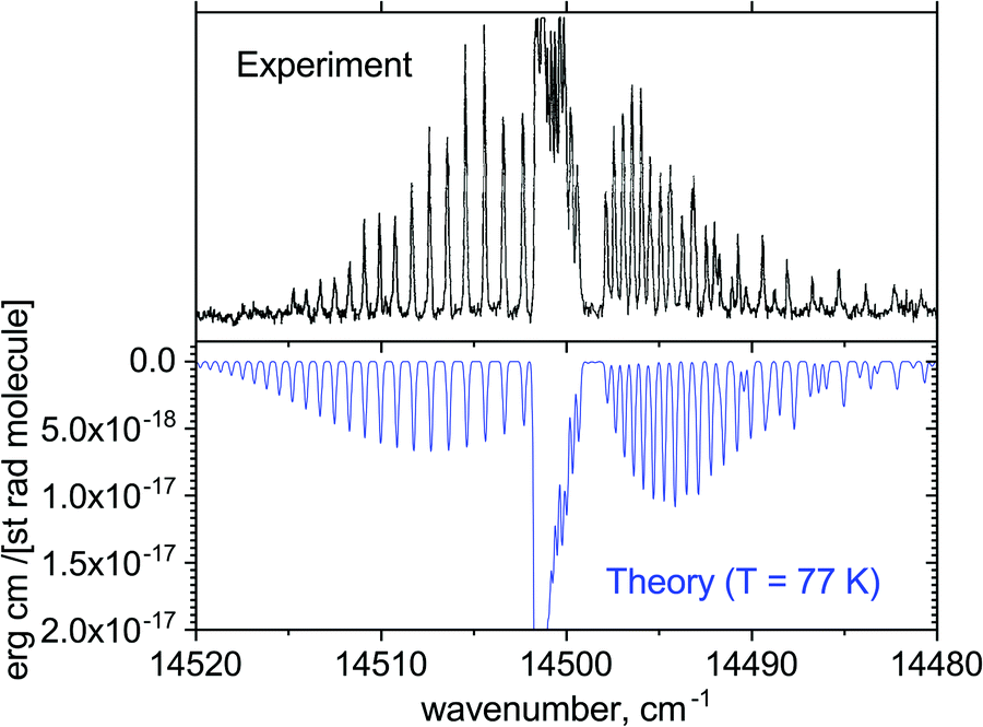
Fig. 14 illustrates the A′²Δ–X²Σ⁺ (0,0) forbidden band in emission simulated for T = 77 K compared to the experimental spectrum of Simard et al.³⁹ Here, a shift of +81.096 cm⁻¹ was applied to the T_e value of the A′²Δ state. In spectral simulations, this region appears to be contaminated by the dipole-allowed hot A–X transitions, which are not necessarily very accurate in this region. We therefore applied a filter to select the A′²Δ–X²Σ⁺ transitions only. The difference in shape of the spectra can be attributed either to the non-LTE (Local Thermal Equilibrium) effects present in the experiment or broadening effects, which we have not attempted to model properly. This figure is only to illustrate the generally good agreement of the positions of the rovibronic lines in this band.

Fig. 14 Comparison of the computed emission A′²Δ–X²Σ⁺ (0,0) band with the measurements of Simard et al.³⁹ at T = 77 K and Gaussian line profile of HWHM = 0.1 cm⁻¹.

Fig. 15 shows a series of absorption bands compared to the measurements of Zhang et al.³⁷ Zhang et al.³⁷ who observed bands in both the B²Σ⁺–X²Σ⁺ and D²Σ⁺–X²Σ⁺ systems in a heavily non-thermal environment where the vibrations were hot and the rotations cooled to liquid nitrogen temperatures. In this case of multi-band system it was important to include at least some non-LTE effects by treating it using two temperatures, vibrational and rotational, assuming that the corresponding degrees of freedom are in LTE. The rotational temperature T_rot = 77 K was set to value specified by Zhang et al.,³⁷ while the vibrational temperature was adjusted to T_vib = 2000 K to better reproduce the experimental spectrum. The spectrum is divided into five spectroscopic windows (I–V) which are also detailed in Table 9. In order to match the positions of the vibronic bands in the experiment, some of the windows were shifted. For example, the D²Σ⁺–X²Σ⁺ (1,0) band was shifted by about 76.5 cm⁻¹. This shift is an indication of the inaccuracy with which our model reproduces the vibrationally excited states of D²Σ⁺. This is not surprising considering the complexity of the quantum-chemistry part of these systems as well as of the nuclear motion part. The avoided crossing with the B²Σ⁺ state leads to very complex shapes of the D²Σ⁺ PEC and of the SO and electronic angular momentum coupling curves with the A and C states. The corresponding SOCs of the B and D states with the nearby state C are also relatively large, ∼30 cm⁻¹ and 80 cm⁻¹, respectively (see Fig. 9), and therefore important. Besides, the D PEC is rather shallow with the equilibrium in the vicinity of the avoided crossing point, which also complicates the solution. An accurate description of the B and D curves would require diabatic representations before attempting any empirical refinement by fitting to the experiment. In all cases our simulations, while not perfect, show striking agreement with the observed spectra.

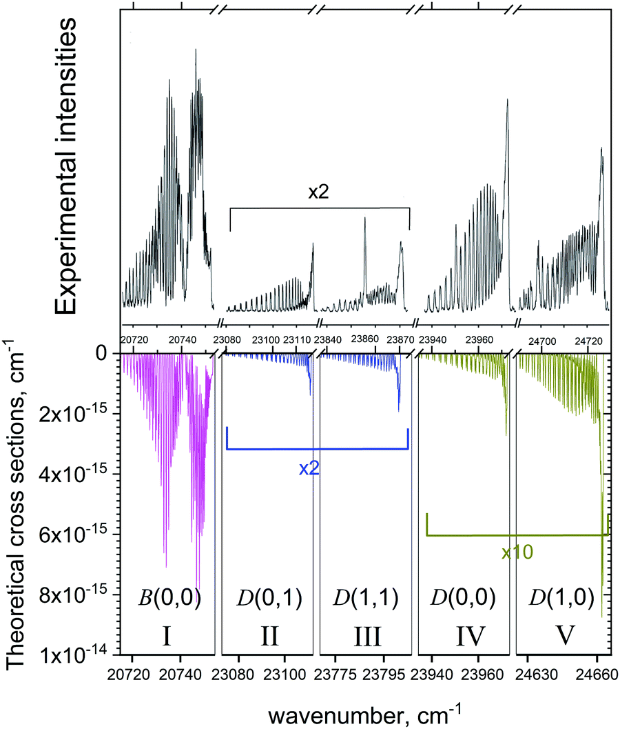Fig. 15 Comparison of our computed emission spectra to the measurements of Zhang et al.³⁷ Our simulations assumed a cold rotational temperature of T_rot = 77 K and a hot vibrational temperature of T_vib = 2000 K. The Gaussian line profile of HWHM = 0.1 cm⁻¹ was used.

Table 9 Five spectroscopic windows (cm⁻¹) used to compare five vibronic bands of YO (B and D) in Fig. 15. Experiment is by Zhang et al.³⁷ while theory is from this work

	Experiment	Theory	Band
I	20714.5–20753.5	20 715–20 754	B(0,0)
II	23078.5–23 117	23 073–23 112	D(0,1)
III	23837.5–23874.5	23 769–23 806	D(1,1)
IV	23934.5–23 973	23934.5–23 973	D(0,0)
V	24 689–24 730	24625.5–24 666	D(1,0)

---

3.5 Lifetimes

The lifetimes of ⁸⁹Y¹⁶O in the A²Π and B²Σ⁺ states (v ≤ 2) were measured by Liu and Parson¹² using laser fluorescence detection of nascent product state distributions in the reactions of Y with O₂, NO, and SO₂. Some lifetimes were also measured by Zhang et al.³⁷ and computed ab initio by Langhoff and Bauschlicher.⁵³Table 10 presents a comparison of these results with our calculations with Duo,⁵⁰ showing value of the states with corresponding lowest J and the positive parity. It can be seen that our A²Π state lifetimes appear to be shorter than the observed ones. This suggests that the A²Π–X²Σ⁺ transition dipoles may be slightly too large. Good agreement is obtained for the lifetimes of the B²Σ⁺ states, while the D²Σ⁺ state lifetimes are underestimated by a factor of 2 indicating that the corresponding transition dipole moments D–B and D–X, or at least one of them might be too large.

Table 10 Lifetimes of ⁸⁹Y¹⁶O states in ns: comparison with the measurements of Liu and Parson¹² and Zhang et al.,³⁷ and the ab initio calculations of Langhoff and Bauschlicher⁵³

State	v	12	37	53	This work
A^2Π1/2	0	33.0 ± 1.3		21	22.7
	1	36.5 ± 2.4			23.0
A^2Π3/2	0	32.3 ± 0.9		21	20.9
	1	30.4 ± 1.8			21.3
	2	33.4 ± 1.5			21.7
	6	41.6 ± 2.1			35.7
B^2Σ^+	0	30.0 ± 0.9	38 ± 5	17	26.7
	1	32.5 ± 1.2			29.2
D^2Σ^+	0		79 ± 5		34.1
	1		79 ± 5		41.4

---

4 Conclusion

In this work, a composite approach to accurate first-principles description of the spectroscopy of open-shell TM-containing diatomics is proposed and its high efficiency is demonstrated taking the example of the yttrium oxide molecule. The approach is based on the combined use of single reference coupled cluster and multireference methods of electronic structure theory, accompanied with a thorough joint analysis of the SR/MR character of the molecular wave function. A full set of potential energy, (transition) dipole moment, spin–orbit, and electronic angular momenta curves for the lowest 6 electronic states of YO was produced ab initio using a combination of the CCSD(T)/CBS and MRCI methods. These curves were then used to solve the fully coupled Schrödinger equation for the nuclear motion using the Duo program. Given the complexity of the system under study, the results show remarkably good agreement with the experiment. Our ultimate goal is to produce an accurate, empirical line list for ⁸⁹Y¹⁶O for applications in modelling the spectroscopy of atmospheres of exoplanets and cool stars. This will require a refinement of the ab initio curves by fitting to the experimental data in the diabatic representation as well as inclusion of the non-adiabatic coupling effects and will be addressed in future work. The A²Π band of YO has strong absorption in the visible region, i.e. where the stellar radiation usually peaks. Such systems are known to cause the temperature inversion in atmospheres of exoplanets, similar to the inversion caused by TiO and VO in giant exoplanets.¹¹³ Opacities of such species are crucial in modelling the degree of temperature inversion in giant exoplanets. YO is yet to be detected in exoplanetary atmospheres and this work is meant to provide the necessary spectroscopic data.

YO is one of the few molecules with the strong potential for laser-cooling techniques,¹⁸ which have widely ranging applications, from quantum information and chemistry to searches for new fundamental physics. The results of this work will help to model the cooling properties of YO and thus will be important for designing and implementing laser-cooling experiments.

The ab initio curves of YO obtained in this study are provided as part of the supplementary material to this paper along with our spectroscopic model in a form of a Duo input file. The computed line list can be obtained from http://www.exomol.com. This is given in the ExoMol format¹⁰⁶ which also includes state-dependent lifetimes. The line list can be directly used with the ExoCross program to simulate the spectral properties of YO.

Conflicts of interest

There are no conflicts to declare.

Acknowledgements

This work was supported by STFC Projects No. ST/M001334/1 and ST/R000476/1. The authors acknowledge the use of the UCL Legion High Performance Computing Facility (Legion@UCL), and associated support services, in the completion of this work, along with the Cambridge COSMOS SMP system, part of the STFC DiRAC HPC Facility supported by BIS National E-infrastructure capital grant ST/P002307/1 and ST/R002452/1 and STFC operations grant ST/R00689X/1. DiRAC is part of the National e-Infrastructure. A. N. S. and V. G. S. acknowledge support from the Ministry of Science and Higher Education of the Russian Federation (Project No. 4.3232.2017/4.6).

References

1. P. F. Bernath, Int. Rev. Phys. Chem., 2009, 28, 681–709.
2. L. K. McKemmish, S. N. Yurchenko and J. Tennyson, Mol. Phys., 2016, 114, 3232–3248.
3. S. A. Cotton, Scandium, Yttrium & the Lanthanides: Inorganic & Coordination Chemistry, John Wiley & Sons, Ltd., 2006.
4. E. Anders and N. Grevesse, Geochim. Cosmochim. Acta, 1989, 53, 197–214.
5. P. S. Murty, Astrophys. Lett. Commun., 1982, 23, 7–9.
6. P. S. Murty, Astrophys. Space Sci., 1983, 94, 295–305.
7. V. P. Goranskii and E. A. Barsukova, Astron. Rep., 2007, 51, 126–142.
8. T. Kaminski, M. Schmidt, R. Tylenda, M. Konacki and M. Gromadzki, Astrophys. J., Suppl. Ser., 2009, 182, 33–50.
9. J. M. Badie, L. Cassan and B. Granier, Eur. Phys. J.: Appl. Phys., 2005, 29, 111–114.
10. J. M. Badie, L. Cassan and B. Granier, Eur. Phys. J.: Appl. Phys., 2005, 32, 61–64.
11. J. M. Badie, L. Cassan and B. Granier, Eur. Phys. J.: Appl. Phys., 2007, 38, 177–181.
12. K. Liu and J. M. Parson, J. Chem. Phys., 1977, 67, 1814–1828.
13. A. Bernard and R. Gravina, Astrophys. J., Suppl. Ser., 1983, 52, 443–450.
14. M. T. Hummon, M. Yeo, B. K. Stuhl, A. L. Collopy, Y. Xia and J. Ye, Phys. Rev. Lett., 2013, 110, 143001.
15. M. Yeo, M. T. Hummon, A. L. Collopy, B. Yan, B. Hemmerling, E. Chae, J. M. Doyle and J. Ye, Phys. Rev. Lett., 2015, 114, 223003.
16. A. L. Collopy, M. T. Hummon, M. Yeo, B. Yan and J. Ye, New J. Phys., 2015, 17, 055008.
17. G. Quéméner and J. L. Bohn, Phys. Rev. A: At., Mol., Opt. Phys., 2016, 93, 012704.
18. A. L. Collopy, S. Ding, Y. Wu, I. A. Finneran, L. Anderegg, B. L. Augenbraun, J. M. Doyle and J. Ye, Phys. Rev. Lett., 2018, 121, 213201.
19. J. B. Shin and R. W. Nicholls, Spectrosc. Lett., 1977, 10, 923–935.
20. C. Linton, J. Mol. Spectrosc., 1978, 69, 351–364.
21. A. Bernard, R. Bacis and P. Luc, Astrophys. J., 1979, 227, 338–348.
22. K. Liu and J. M. Parson, J. Phys. Chem., 1979, 83, 970–973.
23. T. Wijchers, H. A. Dijkerman, P. J. T. Zeegers and C. T. J. Alkemade, Spectrochim. Acta, Part B, 1980, 35, 271–279.
24. S. P. Bagare and N. S. Murthy, Pramana, 1982, 19, 497–499.
25. T. Wijchers, H. A. Dijkerman, P. J. T. Zeegers and C. T. J. Alkemade, Chem. Phys., 1984, 91, 141–159.
26. W. J. Childs, O. Poulsen and T. C. Steimle, J. Chem. Phys., 1988, 88, 598–606.
27. T. C. Steimle and J. E. Shirley, J. Chem. Phys., 1990, 92, 3292–3296.
28. R. Dye, R. Muenchausen and N. Nogar, Chem. Phys. Lett., 1991, 181, 531–536.
29. D. Fried, T. Kushida, G. P. Reck and E. W. Rothe, J. Appl. Phys., 1993, 73, 7810–7817.
30. C. E. Otis and P. M. Goodwin, J. Appl. Phys., 1993, 73, 1957–1964.
31. J. M. Badie and B. Granier, Chem. Phys. Lett., 2002, 364, 550–555.
32. J. M. Badie and B. Granier, Eur. Phys. J.: Appl. Phys., 2003, 21, 239–242.
33. T. Kobayashi and T. Sekine, Chem. Phys. Lett., 2006, 424, 54–57.
34. J. M. Badie, L. Cassan, B. Granier, S. A. Florez and F. C. Janna, J. Sol. Energy Eng., 2007, 129, 412–415.
35. A. Bernard and R. Gravina, Astrophys. J., Suppl. Ser., 1980, 44, 223–239.
36. J. W. H. Leung, T. M. Ma and A. S. C. Cheung, J. Mol. Spectrosc., 2005, 229, 108–114.
37. D. Zhang, Q. Zhang, B. Zhu, J. Gu, B. Suo, Y. Chen and D. Zhao, J. Chem. Phys., 2017, 146, 114303.
38. C. L. Chalek and J. L. Gole, J. Chem. Phys., 1976, 65, 2845–2859.
39. B. Simard, A. M. James, P. A. Hackett and W. J. Balfour, J. Mol. Spectrosc., 1992, 154, 455–457.
40. U. Uhler and L. Akerlind, Ark. Fys., 1961, 19, 1–16.
41. T. C. Steimle and Y. Alramadin, Chem. Phys. Lett., 1986, 130, 76–78.
42. J. Hoeft and T. Torring, Chem. Phys. Lett., 1993, 215, 367–370.
43. P. H. Kasai and W. Weltner, Jr., J. Chem. Phys., 1965, 43, 2553.
44. T. C. Steimle and Y. Alramadin, J. Mol. Spectrosc., 1987, 122, 103–112.
45. R. D. Suenram, F. J. Lovas, G. T. Fraser and K. Matsumura, J. Chem. Phys., 1990, 92, 4724–4733.
46. L. B. Knight, J. G. Kaup, B. Petzoldt, R. Ayyad, T. K. Ghanty and E. R. Davidson, J. Chem. Phys., 1999, 110, 5658–5669.
47. T. C. Steimle and W. Virgo, J. Mol. Spectrosc., 2003, 221, 57–66.
48. D. M. Manos and J. M. Parson, J. Chem. Phys., 1975, 63, 3575–3585.
49. C. L. Chalek and J. L. Gole, Chem. Phys., 1977, 19, 59–90.
50. J. Tennyson, K. Hulme, O. K. Naim and S. N. Yurchenko, J. Phys. B: At., Mol. Opt. Phys., 2016, 49, 044002.
51. A. G. Gaydon, Dissociation Energies and Spectra of Diatomic Molecules, Chapman and Hall, Ltd., London, 3rd edn, 1968.
52. R. J. Ackermann and E. G. Rauh, J. Chem. Phys., 1974, 60, 2266–2271.
53. S. R. Langhoff and C. W. Bauschlicher, J. Chem. Phys., 1988, 89, 2160–2169.
54. P. Sriramachandran and R. Shanmugavel, New Astron., 2011, 16, 110–113.
55. J. Tennyson and S. N. Yurchenko, Mon. Not. R. Astron. Soc., 2012, 425, 21–33.
56. L. Lodi, S. N. Yurchenko and J. Tennyson, Mol. Phys., 2015, 113, 1559–1575.
57. L. K. McKemmish, S. N. Yurchenko and J. Tennyson, Mon. Not. R. Astron. Soc., 2016, 463, 771–793.
58. L. K. McKemmish, T. Masseron, J. Hoeijmakers, V. V. Pérez-Mesa, S. L. Grimm, S. N. Yurchenko and J. Tennyson, Mon. Not. R. Astron. Soc., 2019, 488, 2836–2854.
59. J. F. Stanton and J. Gauss, Adv. Chem. Phys., 2003, 125, 101–146.
60. J. Tennyson, L. Lodi, L. K. McKemmish and S. N. Yurchenko, J. Phys. B: At., Mol. Opt. Phys., 2016, 49, 102001.
61. Ľ. Horný, A. Paul, Y. Yamaguchi and H. F. Schaefer III, J. Chem. Phys., 2004, 121, 1412–1418.
62. C. Puzzarini and K. A. Peterson, J. Chem. Phys., 2005, 122, 084323.
63. A. Paul, Y. Yamaguchi, H. F. Schaefer III and K. A. Peterson, J. Chem. Phys., 2006, 124, 034310.
64. A. Paul, Y. Yamaguchi and H. F. Schaefer III, J. Chem. Phys., 2007, 127, 154324.
65. S. N. Yurchenko, L. Lodi, J. Tennyson and A. V. Stolyarov, Comput. Phys. Commun., 2016, 202, 262–275.
66. H.-J. Werner and P. J. Knowles, J. Chem. Phys., 1988, 89, 5803–5814.
67. P. J. Knowles and H.-J. Werner, Chem. Phys. Lett., 1988, 145, 514–522.
68. P. J. Knowles and H.-J. Werner, Theor. Chem. Acc., 1992, 84, 95–103.
69. H.-J. Werner and P. J. Knowles, J. Chem. Phys., 1985, 82, 5053–5063.
70. P. J. Knowles and H.-J. Werner, Chem. Phys. Lett., 1985, 115, 259–267.
71. K. A. Peterson, D. Figgen, M. Dolg and H. Stoll, J. Chem. Phys., 2007, 126, 124101.
72. R. A. Kendall, T. H. Dunning and R. J. Harrison, J. Chem. Phys., 1992, 96, 6796–6806.
73. T. Shiozaki, W. Györffy, P. Celani and H.-J. Werner, J. Chem. Phys., 2011, 135, 081106.
74. K. A. Peterson and T. H. Dunning, J. Chem. Phys., 2002, 117, 10548.
75. A. Berning, M. Schweizer, H.-J. Werner, P. J. Knowles and P. Palmieri, Mol. Phys., 2000, 98, 1823–1833.
76. L. Visscher, Theor. Chem. Acc., 1997, 98, 68–70.
77. K. G. Dyall, J. Chem. Phys., 1994, 100, 2118–2127.
78. K. G. Dyall, Theor. Chem. Acc., 2007, 117, 483–489.
79. K. G. Dyall, Theor. Chem. Acc., 2016, 135, 128.
80. A. Shee, T. Saue, L. Visscher and A. S. P. Gomes, J. Chem. Phys., 2018, 149, 174113.
81. A. Kramida, Yu. Ralchenko, J. Reader and NIST ASD Team, NIST Atomic Spectra Database (ver. 5.6.1), [Online]. Available: https://physics.nist.gov/asd [2019, April 13]. National Institute of Standards and Technology, Gaithersburg, MD., 2019.
82. C. Hampel, K. A. Peterson and H.-J. Werner, Chem. Phys. Lett., 1992, 190, 1–12.
83. J. D. Watts, J. Gauss and R. J. Bartlett, J. Chem. Phys., 1993, 98, 8718–8733.
84. P. J. Knowles, C. Hampel and H. J. Werner, J. Chem. Phys., 1993, 99, 5219–5227.
85. J. M. L. Martin, Chem. Phys. Lett., 1996, 259, 669–678.
86. A. Karton and J. M. L. Martin, Theor. Chem. Acc., 2006, 115, 330–333.
87. K. A. Peterson, D. Woon and T. H. Dunning, J. Chem. Phys., 1994, 100, 7410–7415.
88. J. L. Dunham, Phys. Rev., 1932, 41, 721–731.
89. H. J. Werner, P. J. Knowles, G. Knizia, F. R. Manby, M. Schütz, P. Celani, W. Györffy, D. Kats, T. Korona, R. Lindh, A. Mitrushenkov, G. Rauhut, K. R. Shamasundar, T. B. Adler, R. D. Amos, A. Bernhardsson, A. Berning, D. L. Cooper, M. J. O. Deegan, A. J. Dobbyn, F. Eckert, E. Goll, C. Hampel, A. Hesselmann, G. Hetzer, T. Hrenar, G. Jansen, C. Köppl, Y. Liu, A. W. Lloyd, R. A. Mata, A. J. May, S. J. McNicholas, W. Meyer, M. E. Mura, A. Nicklass, D. P. O'Neill, P. Palmieri, D. Peng, K. Pflüger, R. Pitzer, M. Reiher, T. Shiozaki, H. Stoll, A. J. Stone, R. Tarroni, T. Thorsteinsson and M. Wang, MOLPRO, version 2015.1, a package of ab initio programs, http://www.molpro.net, 2015.
90. DIRAC, a relativistic ab initio electronic structure program, Release DIRAC18, written by T. Saue, L. Visscher, H. J. Aa. Jensen, and R. Bast, with contributions from V. Bakken, K. G. Dyall, S. Dubillard, U. Ekström, E. Eliav, T. Enevoldsen, E. Faßhauer, T. Fleig, O. Fossgaard, A. S. P. Gomes, E. D. Hedegård, T. Helgaker, J. Henriksson, M. Iliaš, Ch. R. Jacob, S. Knecht, S. Komorovský, O. Kullie, J. K. Lærdahl, C. V. Larsen, Y. S. Lee, H. S. Nataraj, M. K. Nayak, P. Norman, G. Olejniczak, J. Olsen, J. M. H. Olsen, Y. C. Park, J. K. Pedersen, M. Pernpointner, R. di Remigio, K. Ruud, P. Sałek, B. Schimmelpfennig, A. Shee, J. Sikkema, A. J. Thorvaldsen, J. Thyssen, J. van Stralen, S. Villaume, O. Visser, T. Winther, and S. Yamamoto, 2018, available at https://doi.org/10.5281/zenodo.2253986, see also http://www.diracprogram.org.
91. J. Tennyson and S. N. Yurchenko, Int. J. Quantum Chem., 2017, 117, 92–103.
92. A. T. Patrascu, C. Hill, J. Tennyson and S. N. Yurchenko, J. Chem. Phys., 2014, 141, 144312.
93. S. N. Yurchenko, I. Szabo, E. Pyatenko and J. Tennyson, Mon. Not. R. Astron. Soc., 2018, 480, 3397–3411.
94. H.-Y. Li, J. Tennyson and S. N. Yurchenko, Mon. Not. R. Astron. Soc., 2019, 486, 2351–2365.
95. T. J. Lee and P. R. Taylor, Int. J. Quantum Chem., 1989, 36, 199–207.
96. C. L. Janssen and I. M. B. Nielsen, Chem. Phys. Lett., 1998, 290, 423–430.
97. W. Jiang, N. J. DeYonker and A. K. Wilson, J. Chem. Theory Comput., 2012, 8, 460–468.
98. J. Wang, S. Manivasagam and A. K. Wilson, J. Chem. Theory Comput., 2015, 11, 5865–5872.
99. A. Karton, E. Rabinovich, J. M. L. Martin and B. Ruscic, J. Chem. Phys., 2006, 125, 144108.
100. A. Karton, S. Daon and J. M. L. Martin, Chem. Phys. Lett., 2011, 510, 165–178.
101. J. Shirley, C. Scurlock and T. Steimle, J. Chem. Phys., 1990, 93, 1568–1575.
102. C. W. Bauschlicher and S. R. Langhoff, J. Chem. Phys., 1986, 85, 5936–5942.
103. T. C. Steimle and W. Virgo, J. Chem. Phys., 2002, 116, 6012–6020.
104. R. Stringat, C. Athénour and J. L. Féménias, Can. J. Phys., 1972, 50, 395–403.
105. A. Bernard and J. Vergés, J. Mol. Spectrosc., 2000, 201, 172–174.
106. J. Tennyson, S. N. Yurchenko, A. F. Al-Refaie, E. J. Barton, K. L. Chubb, P. A. Coles, S. Diamantopoulou, M. N. Gorman, C. Hill, A. Z. Lam, L. Lodi, L. K. McKemmish, Y. Na, A. Owens, O. L. Polyansky, T. Rivlin, C. Sousa-Silva, D. S. Underwood, A. Yachmenev and E. Zak, J. Mol. Spectrosc., 2016, 327, 73–94.
107. S. N. Yurchenko, A. F. Al-Refaie and J. Tennyson, Astron. Astrophys., 2018, 614, A131.
108. C. M. Western, J. Quant. Spectrosc. Radiat. Transfer, 2017, 186, 221–242.
109. R. R. Reddy, Y. Nazeer Ahammed, K. Rama Gopal, P. Abdul Azeem and S. Anjaneyulu, Astrophys. Space Sci., 1998, 262, 223–240.
110. P. S. Barklem and R. Collet, Astron. Astrophys., 2016, 588, A96.
111. R. R. Gamache, C. Roller, E. Lopes, I. E. Gordon, L. S. Rothman, O. L. Polyansky, N. F. Zobov, A. A. Kyuberis, J. Tennyson, S. N. Yurchenko, A. G. Császár, T. Furtenbacher, X. Huang, D. W. Schwenke, T. J. Lee, B. J. Drouin, S. A. Tashkun, V. I. Perevalov and R. V. Kochanov, J. Quant. Spectrosc. Radiat. Transfer, 2017, 203, 70–87.
112. M. S. Vardya, Astron. Astrophys., 1970, 5, 162–164.
113. N. Madhusudhan and S. Gandhi, Mon. Not. R. Astron. Soc., 2017, 472, 2334–2355.

---

Footnote

† Electronic supplementary information (ESI) available. See DOI: 10.1039/c9cp03208h

---