Investigation of the properties of nanographene in polymer nanocomposites through molecular simulations: dynamics and anisotropic Brownian motion

Abstract

The dynamical behavior of nanographene sheets dispersed in polymer matrices is investigated through united-atom molecular dynamics simulations. The Brownian motion of the sheet and the anisotropy in its translational and orientational diffusion are the topics of the current study. Different polymer matrices and pristine and functionalized graphene constitute various nanocomposite systems. Interactions between the nanographene flake and the matrix determine the dynamics of the systems. The dynamics is reduced in polyethylene oxide compared to polyethylene matrix, whereas carboxylated sheets move considerably slower than the pristine nanographene in any matrix. Diffusion is anisotropic for short times, while it becomes isotropic in the long time limit. The in-plane motion of the nanographene sheet is faster than the out-of-plane component, in agreement with the diffusion of perfectly oblate ellipsoids. In functionalized graphene, the anisotropy is suppressed. By exploring the temperature effect on both the nanographene sheet and polymer close to the surface, indications for coupling in the motion of the two components are revealed. The strong effect of edge functional groups on the dynamics can be used as a way to control the Brownian motion of nanographene sheets in polymer nanocomposites and consequently tailor the properties of the materials.

---

1. Introduction

Since the seminal work by A. Einstein, the concept of Brownian motion^1,2 has been widely used in physics, chemistry, mathematics and other sciences. The Brownian motion (BM) of small isotropic particles moving in a fluid is nowadays well-defined, and extensively investigated through theory,^3–5 simulations⁶ and experiments.^7,8 For spherical particles diluted in a Newtonian fluid, dynamics and hydrodynamics are isotropic following the typical Stokes–Einstein relation.^9,10 However, the Brownian motion of non-spherical particles, as well as of particles moving in a viscoelastic medium, is much more complicated, exhibiting clear anisotropic features and usually long-term non-linear (anomalous) effects.

In the current study the Brownian motion of nanographene flakes in polymer matrices is investigated. Graphene is a two-dimensional monolayer of graphite of macroscopic dimensions but of atomic thickness, which was first isolated in 2004.¹¹ Nowadays, there is enormous interest in the study of graphene-based nanostructured materials, due to the exceptional physical properties of graphene (e.g., electronic, optical, thermal, and mechanical properties),^11–15 which make it a candidate material for a wide range of potential applications.^16–20 In polymer nanocomposites graphene sheets are used as nanofillers^21–25 in order to enhance their mechanical and functional properties.

The conformational and dynamical properties of nanographene in a polymer matrix can be of particular importance. Indeed, both the conformational transitions (rippling or wrinkling) and the mobility of the graphene nanofiller in the composite can strongly affect the properties of the whole material;^26–30 however, there is no obvious correlation between them. For example, it has been observed that both these factors inhibit adsorption of polymer on the surface of a graphene flake in polyethylene/graphene nanocomposites, resulting in a lower density of polymer at the interface, compared to the case of a frozen sheet.^31,32 Furthermore, the strong effect on the electronic properties of graphene^30,33 and increased chemical reactivity and change in charge distribution^34,35 have been attributed to rippling.

Rubinstein and coworkers^36,37 have explored the way that a polymer melt affects the motion of a spherical nanoparticle through scaling theory and molecular dynamics simulations. This is found to be related to the correlation between the diameter of the nanoparticle (d) and the structural length scales of polymers (i.e., spacings between polymer entanglements) (a). The mobility of the nanoparticle is enhanced for d < a, remains almost unchanged for d ≈ a and is suppressed for d > a.

For a 2D flake, anisotropic Brownian particle dynamics has been detected experimentally through optical trapping of individual graphene flakes in water.³⁸ The study of the Brownian motion of ellipsoidal particles in water reveals an anisotropic diffusion for short times, which becomes isotropic for longer times. The coupling between the rotational and translational motion of the ellipsoids was illustrated with the use of digital video microscopy.³⁹ Furthermore, the motion of perfectly rigid prolate ellipsoids dispersed in a sea of spheres has been investigated through molecular dynamics simulations using simple bead–spring models.⁴⁰ It was found that there is anisotropy in the motion of the ellipsoids for short up to intermediate times, where the motion of the molecules is faster in the direction parallel to their long (major) axis compared to the perpendicular direction, characterized as needlelike motion. An opposite behavior is observed for oblate ellipsoids, where the correlation between the two components of the mean squared displacement is reverse (i.e., faster perpendicular and slower parallel components with respect to the major axis).⁴¹ In both cases for long times the diffusion becomes isotropic.

In the present work we study the (anisotropic) Brownian motion of small graphene sheets (nanographene) in different environments. Since there is no accurate theoretical description of the dynamics of a fluctuating 2D material in a polymeric (viscoelastic) medium, we have used predictions from simpler models, concerning the diffusion of non-spherical objects in a Newtonian liquid, and more specifically of oblate ellipsoids; nanographene flakes are expected to be, approximately, described by such a shape.

The current study highlights the dynamics of nanographene flakes well-dispersed in polymer matrices. Both different polymers and different kinds of nanofillers (i.e., pristine and functionalized graphene sheets of various sizes) have been examined. In general, this is a complicated issue since the dynamics is expected to depend on several factors, such as the size and the shape of the sheet, the functional groups at edges, and the strength of the graphene/polymer interactions. In all cases model graphene flakes are of rather small areas (nm dimensions); therefore, the term nanographene is used. The goal of the present study is to reveal information about the (anisotropic) dynamical behavior of nanographene on the atomic scale. The effects of different host matrices, types of nanographene sheets and temperatures on the dynamics of the sheet are presented. The translational and rotational motions of nanographene are examined in both parallel and perpendicular directions to the graphene plane. The anisotropic dynamical behavior of the nanographene sheet, induced by its 2D geometry and its conformational transitions, are also detected. Moreover, a coupling between the motions of the nanographene flake and the polymer layer in its vicinity is investigated.

The rest of the paper is organized as follows: in Section 2 we briefly discuss the basic theoretical concepts of anisotropic Brownian motion. In Section 3 details about the model systems, the simulations, and the analysis procedure are given. The Results and discussion section separated into subsections according to the individual parameters under investigation are presented in Section 4. Conclusions follow in Section 5.

2. Anisotropic Brownian motion

(A) Steady state regime

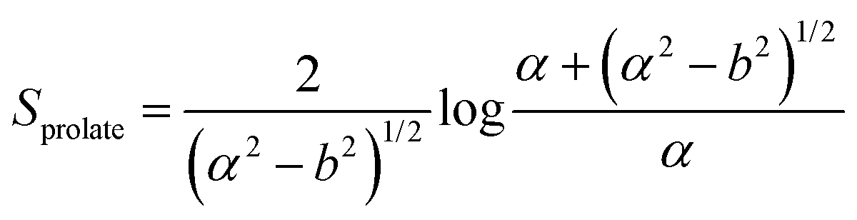
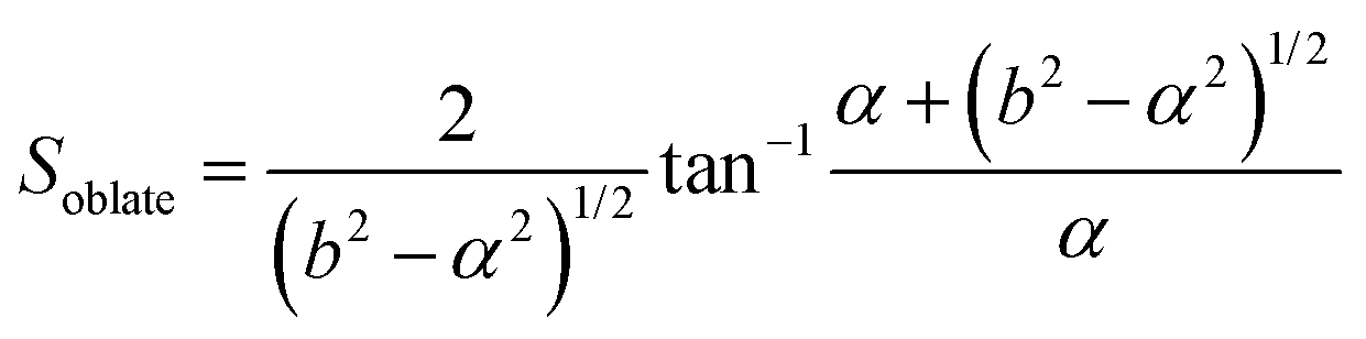
In this section, theoretical predictions for the translational Brownian motion (BM) of anisotropic particles are briefly outlined. The dynamics of isotropic spherical particles embedded in a viscous fluid is described by the well-known Stokes–Einstein relation: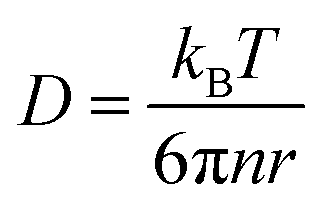 , where D is the diffusion coefficient of the particle, k_B the Boltzmann constant, n the dynamic viscosity of the matrix and r the radius of the spherical particle. For particles of anisotropic shape, a modification of this relation is based on the solution of the Navier–Stokes hydrodynamic equations. For ellipsoids, anisotropy implies the study of motion in two directions: one parallel to their major axis and one perpendicular to it. The predictions for the corresponding diffusion coefficients for both prolate (rod-like) and oblate ellipsoids are as follows:⁴²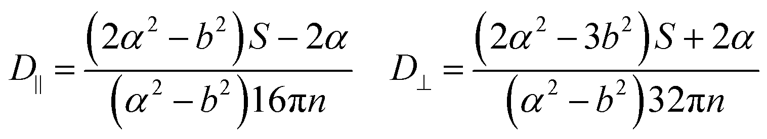where α and b are the lengths of the semi-major and semi-minor axes of the ellipsoid, respectively. A schematic representation of a perfectly oblate ellipsoid is depicted in Fig. 1c.

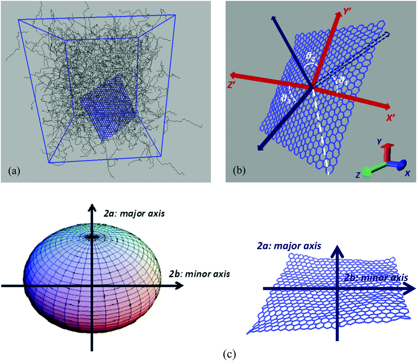Fig. 1 (a) A characteristic configuration of a model nanographene/polymer nanocomposite. (b) Lab frame and body frame representations. Direction cosines formed between the system of axes, defined on the body frame of the initial configuration of graphene, and an instantaneous system of axes, which corresponds to another configuration (body frame) (X′Y′Z′). (c) Schematic representations of a perfectly oblate ellipsoid and a graphene sheet (definitions of the major and minor axes).

There is a big controversy about the solutions of the Navier–Stokes hydrodynamic equations depending on the boundary conditions which are applied. According to the stick hydrodynamic boundary conditions, D_‖ is two times faster than D_⊥ for rods and the predictions are almost identical for a prolate ellipsoid, for the aspect ratios (κ) greater than 2 (κ = L/b, with L the length and b the diameter of the rod). The use of slip hydrodynamic boundary conditions predicts that the motion along the parallel direction can be decoupled from that along the perpendicular direction and the D_‖/D_⊥ ratio approaches κ for large κ-values. This applies to both prolate and oblate ellipsoids.⁴¹

Vasanthi et al.^40,41 presented results of molecular dynamics simulations, using bead–spring models, which show a linear variation of D_‖/D_⊥ with κ, supporting the slip hydrodynamic boundary conditions. According to their findings, anisotropy is observed for long times, in the case of oblates with the motion normal to the major axis (D_⊥) being much faster than the one parallel to the major axis (D_‖). The trend was opposite for prolate ellipsoids and anisotropy was shown for much shorter time scales.

Nanographene's shape is approximately described by an oblate ellipsoid, as is briefly described in the ESI,† (Table SI-1). Therefore, keeping the convention of Fig. 1c, the major axis corresponds to the Z′-direction. Then the corresponding notation in our calculations is −X′Y′ for motion normal to the major axis and −Z′ for motion parallel to the major axis.

(B) Time dependent regime

The above discussion concerns the BM of particles in the long time (steady-state) regime by defining a time independent diffusion coefficient, D. D can be directly related to the molecular (particle) scale via the corresponding Green–Kubo relation:
where v(t) and v(0) are the velocities of a particle at times 0 and t, respectively, and 〈v(t)·v(0)〉 is their autocorrelation function. R(0) and R(t) are the positions of a particle at times 0 and t.

If we also consider the short time regime, then an effective time dependent diffusion coefficient, D(t), can be defined as:

where ΔR² = 〈(R(t) − R(0))²〉 is the mean squared displacement (MSD). D(t) reaches a constant value when MSD scales linearly with time, i.e., ΔR² ∼ t¹. However, this is not the case in the short time regime, where ΔR² ∼ t^c, with c ≠ 1. In general, the dynamics of particles in a medium can be described in different time regimes according to the exponent c: (a) c = 2 represents the (short time) ballistic regime, (b) c < 1 represents the sub-diffusive (anomalous) regime, and (c) c = 1 describes the linear, steady state, regime (Fickian diffusion). In the typical BM of a spherical particle in a medium the dynamical behavior of the particle accesses the different time regimes (i.e., from ballistic to linear) as time increases.

For an anisotropic particle, following the discussion in the previous subsection, we can further define the components of the time dependent diffusion coefficient as and , where (ΔR²)_Z′ and (ΔR²)_X′Y′ are the components of the mean squared displacement for motion parallel and normal to the major axis, respectively. For the motion normal to the major axis the X′ and Y′ directions are equivalent, so their average is used.

3. Simulation method and systems

(A) Model systems

Hybrid nanographene/polymer systems have been simulated through detailed atomistic molecular dynamics simulations. Nanocomposites are comprised of two different polymer matrices, polyethylene (PE) and polyethylene oxide (PEO). Pristine and functionalized nanographene sheets have been used as nanofillers, with two types of functional groups, which are attached only to the edge carbon atoms; (a) hydrogenated graphene, with hydrogen atoms at the edges, and (b) carboxylated graphene, where hydrogens and carboxyl groups are attached randomly to the edges. Graphene is usually produced by the chemical reduction of graphene oxide. Through this method most of the functional groups are removed from the surface of graphene oxide, whereas more edge functional groups remain. The amount of hydrogen atoms which are randomly distributed at the edges of the hydrogenated graphene flake is 8.7%. In the carboxylated graphene 2.9% hydrogens and 5.8% carboxyl groups are attached at the edges. The amount of carboxyl groups in the carboxylated sheet and the respective percentage of the remaining oxygen in graphene correspond to the experimentally observed value of 12.68 wt%.⁴³ Our model consists of a single graphene layer in a polymer matrix, which corresponds to an ideal system of well-dispersed nanocomposites. The percentages of graphene sheets in the polymer matrix are about 3 wt% for pristine graphene and between 1.7 and 3.6 wt% for the functionalized sheets. These values are close to the typical graphene concentration values in graphene-based polymer nanocomposites.⁴⁴

United-atom models are used for both polymers, whereas an all-atom description is used for graphene flakes. For PE and PEO the TraPPE force field⁴⁵ has been used, which has been slightly modified in the case of PEO.⁴⁶ TraPPE has been widely used in the literature for both PE and PEO simulations,^31,32,47 leading to reliable results that compare fairly well with existing experimental data.⁴⁸ For PEO 1620 10-mer polymer chains and for PE 1336 22-mer polymer chains were simulated. The sizes (end-to-end vectors) of both PEO and PE chains are about 18–20 Å, and their radii of gyration are about ∼6.5 Å at 450 K. Concerning the model graphene sheets, we applied a force field previously used for various carbon structures,^49,50 which has been developed through ab initio calculations. For the functional groups grafted onto the graphene edges, since there are no available quantum data, we have chosen the OPLS-AA force field.⁵¹ OPLS-AA is a quite general force field widely used in the description of charged groups. Nanographene sheets of three different dimensions have been simulated in order to estimate the size effect on the various properties under investigation. In all cases the sheet is almost quadratic. A detailed description of the systems, as well as of the atomistic force field, used to describe interactions for both polymer matrices and graphene flakes, is given in the ESI.† All simulated systems are presented in Table 1 and a characteristic configuration of a model nanographene/polymer nanocomposite is depicted in Fig. 1a. The acronyms of our systems are as follows: G stands for graphene, H/COOH subscripts denote the hydrogenated/carboxylated flakes, respectively, and the type of polymer matrix follows after ‘/’. In the case of pristine graphene the subscripts of (G) denote the different areas of the sheet.

Table 1 Description of all model systems studied here

Acronym	Atoms of graphene	System	T (K)	Simulated time (ns)
Pristine graphene/PE
G20/PE	190	Graphene (19 × 20) Å^2/PE	450	100
G50/PE	1032	Graphene (49 × 51) Å^2/PE	450	100
G80/PE	2546	Graphene (84 × 86) Å^2/PE	450	100
Functionalized graphene (49 × 51) Å^2
GH/PE	1122	Graphene-H/PE	450	100
GCOOH/PE	1302	Graphene-COOH/PE	450	200
GH/PEO	1122	Graphene-H/PEO	450	200
GCOOH/PEO	1302	Graphene-COOH/PEO	450	300
(GCOOH/PEO)400	1302	Graphene-COOH/PEO	400	300
(GCOOH/PEO)370	1302	Graphene-COOH/PEO	370	300
(GCOOH/PEO)340	1302	Graphene-COOH/PEO	340	300
(GCOOH/PEO)318	1302	Graphene-COOH/PEO	318	300

---

Molecular dynamics simulations were performed in the isothermal–isobaric (NPT) statistical ensemble at a constant pressure of 1 atm. The integration time step was either 1 fs or 2 fs, depending on the system (i.e., systems with functionalized graphene sheets are simulated with a smaller time step, due to the high vibrational frequency of bonds between edge groups and graphene atoms). All bonds were constrained using the LINCS algorithm.⁵² All the systems were first equilibrated and then followed by production runs, the time of which varies for the different systems between 100 ns and 300 ns as shown in Table 1. Configurations were saved every 50 ps. The temperature for the PE/graphene systems was kept constant using the stochastic velocity rescaling algorithm,⁵³ while in the case of the PEO/graphene ones the Nosé–Hoover thermostat was used.⁵⁴ The time constant for temperature coupling was 0.2 ps for the stochastic velocity rescaling thermostat and 2.5 ps for the Nosé–Hoover thermostat. Correspondingly, the Berendsen barostat, with a time constant of 0.5 ps, and the Parrinello–Rahman barostat, with a time constant of 5 ps, were used. The Coulomb cutoff scheme was applied to the nonpolar matrix, and the particle-mesh Ewald (PME) electrostatics was present in PEO composites. For further details about the model and simulation procedure the reader is referred to the ESI† and our previous work.⁴⁷ Finally, the G_COOH/PEO system was studied at different temperatures in the range of 318–450 K. Note also that for all the systems multiple (from 2 up to 4) simulations, starting with different uncorrelated initial configurations, were performed to improve statistics.

(B) Analysis of model configurations

Our main goal is to study the translational and orientational (anisotropic) Brownian dynamics of nanographene dispersed in the polymer matrix. To achieve this, we perform a detailed analysis, in both the lab and the body frame. The lab frame is defined as the original Cartesian system of coordinates (x, y, z), which is represented by the system of axes shown on the top left corner of Fig. 1b. For our calculations in the body frame the following procedure is performed: first, the optimal plane is defined as the best planar fit to the rippled nanographene sheet. Then, as the body frame, we define a system of axes which lies on the nanographene flake at its instantaneous position (X′Y′Z′) (Fig. 1b). The axes are defined by three atoms: (a) the middle atom of the sheet, (b) the middle atom of the one zigzag edge of the sheet, and (c) the corresponding middle atom of the armchair edge of the sheet. The vector from atom (a) to (b) defines the x-axis, and the vector from (a) to (c) the y-axis, whereas the third axis is defined as the one normal to the plane of the first two. For the above vectors the coordinates of atoms projected onto the optimal plane are used. Therefore, in the following we will refer to the position of the center of mass of the flake or to the components of a measured quantity according to the coordinate system used for their measurement (i.e., x, y, z for the lab frame and X′, Y′, Z′ for the body frame).

Translational Brownian motion (BM) is examined via the calculation of the mean squared displacement (MSD) of the nanographene sheet, in the body frame, as follows:

(a) Given a set of nanographene's snapshots, we define, for each configuration, an instantaneous reference coordinate system, X′Y′ and Z′, as discussed above.

(b) Then, the coordinates of all atoms of the rest of the trajectory are projected onto the instantaneous reference system.

(c) MSD X′Y′ and Z′ components are calculated with respect to the body frame of a given configuration for all subsequent times. The two components X′ and Y′ represent motion normal to the major axis (see Fig. 1c and the corresponding discussion), whereas the component Z′ describes motion parallel to the major axis.

Orientational motion is also analyzed in the body frame, by defining the three Eulerian angles which are formed in the body frame system of axes, between the initial and a given configuration. These angles express the direction cosines between two sets of axes, as is shown in Fig. 1b. Two angles describe the rotation of the graphene flake around an axis perpendicular to the graphene optimal plane (Z′) (rotation, θ₁, θ₂) and one angle represents the rotation around an axis parallel to the plane (X′ or Y′) (rotation, θ₃).

In all the above cases, the multiple time origin technique has been used to improve statistics.

4. Results and discussion

In the following we present simulation results concerning the dynamics of pristine and functionalized graphene sheets dispersed in different polymer matrices.

(A) Dynamics in the lab frame

First, we examine the overall dynamics of the graphene sheets (i.e., averaged over all the (x-, y-, and z-) directions), analyzed in the lab (Cartesian) frame.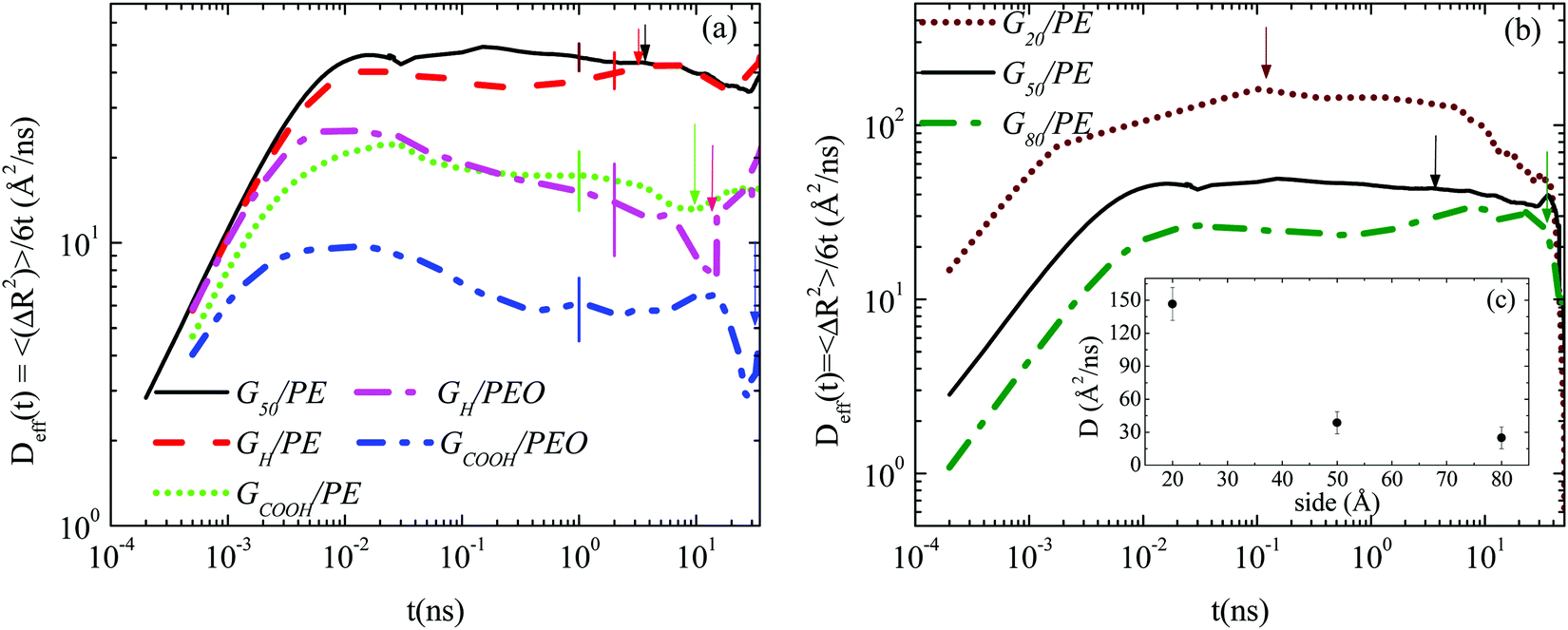

Translational dynamics. The mean squared displacement (MSD), ΔR² = 〈(R(t) − R(0))²〉, of the center of mass of the graphene flake is calculated. As discussed in Section 2B for a homogeneous molecular system, an effective time dependent self-diffusion coefficient can be defined as: D_eff(t) ≡ ΔR²/6t. The results for the D_eff(t) of the nanographene sheets are presented in Fig. 2 as a function of time. Data have been averaged over 2 to 4 independent runs (depending on the system) to improve statistics. For all the systems a plateau-like regime (i.e., c = 1) is observed, which indicates linear (Fickian) diffusion of the flake in the matrix. Moreover, important observations arise from the data reported in Fig. 2a. (a) The dynamics of graphene flakes is reduced in the PEO matrix compared to the PE one, for both hydrogenated and carboxylated graphene sheets. It should be mentioned here that the difference in the T_g-values between the two polymers has a partial effect on this phenomenon. If we define a relative temperature as the difference between the simulation temperature (450 K) and the glass transition temperature of the corresponding bulk system, reported in experiments, (T* = T − T_g) for both polymers, we find that for PE composites T* ≈ 320 K (T_g(PE) ≈ 130 K⁵⁵), whereas for PEO T* ≈ 244 K (T_g(PEO) ≈ 206 K⁵⁶); therefore, PE systems are simulated at higher relative temperature. (b) The carboxylated sheets move considerably more slowly (i.e., ∼1.5–2.5 times) than the hydrogenated ones and the pristine graphene. This difference can be attributed to the difference in mass between the two nanographene sheets and is also related to the higher friction at the edges due to the interaction of carboxyl groups with polymer chains.⁴⁷ (c) The dynamics of the pristine and the hydrogenated graphene in the PE matrix are very similar as expected. The above observations highlight the effect of the electrostatic interactions between the polar PEO matrix and the end groups of the functionalized graphene sheets which are stronger in the case of the carboxyl end groups.

Fig. 2 The effective diffusion coefficient, D_eff(t), of the center of mass of the graphene flake as a function of time at T = 450 K. (a) Systems with graphene flakes of the same size. Representative error bars are shown on each curve. (b) Systems with graphene flakes of different sizes. Arrows point to τ_trans values for the systems. (c) Diffusion coefficient as a function of the size of the graphene sheet.

The factors that mainly affect the dynamics of the nanographene sheets in the nanocomposite are the size of the sheet (Table 1), the polymer/graphene interaction, and the different zero-shear viscosities of the two polymer matrices. In order to examine the latter, we provide a rough estimation for the zero-shear viscosity of the polymer matrix assuming Rouse dynamics. In more detail, the zero-shear rate viscosity of the polymer chains is computed via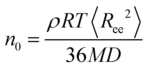, where ρ is the mass density of the bulk system, M is the molecular weight of the polymer, R is the gas constant, T is the temperature, 〈R_ee²〉 is the mean squared end-to-end distance of the chains in the bulk and D is the self-diffusion coefficient of the center of mass of the chain.³² The values obtained for n₀ are 2.35 × 10⁻⁴ P and 8.70 × 10⁻³ P for PE and PEO respectively.

Fig. 2b depicts the mean squared displacement, scaled with 6t (time dependent effective diffusion coefficient), for the three nanocomposites of PE with pristine graphene flakes of different sizes (G₂₀/PE, G₅₀/PE, G₈₀/PE). As expected, the smaller the sheet the faster its translational motion in the polymer matrix.³¹ In Fig. 2c (inset of Fig. 2b) the diffusion coefficient (D) is presented as a function of the size of the sheet. Values are extracted as a rough estimation of the plateau region of the curves. Not surprisingly, the dynamics of (single-sheet) well dispersed nano-graphene layers is rather noisy; however, a clear decrease of D with size is observed, which has a difference of almost one order of magnitude between the smallest sheet and the largest sheet.

Furthermore, from the data of Fig. 2 one can extract a characteristic time for the translational motion of the nanographene flakes. We define τ_trans as the time during which a graphene sheet moves a distance equal to the half of its size, in one direction (e.g., 〈ΔR²〉 ∼ (25 Å)² for G₅₀). The corresponding values are also depicted in Table 2 and indicated with arrows in Fig. 2. Based on τ_trans, it is interesting to observe that the graphene flakes in the PEO nanocomposites are almost 4 times slower for both hydrogenated and carboxylated sheets compared to those in the PE nanocomposites. Moreover, the carboxylated sheets are almost ∼2.5 times slower than the hydrogenated ones in both polymers.

Table 2 Characteristic times for the translational diffusion, τ_trans, and orientational relaxation times, τ_orient, with the associated stretch exponents, β, for the nano-graphene sheets in the various polymer nanocomposites studied here

System	τ trans (ns) ± ∼(20%)	τ orient (ns) ± ∼(20%)	β ± ∼0.05
G50/PE	3.5	8.92	0.83
GH/PE	3.4	9.42	0.79
GCOOH/PE	9.4	13.13	1
GH/PEO	13.5	25.07	0.85
GCOOH/PEO	31.5	48.96	1
GH/PE(80mer)	10.5	25.32	1

---

Summing up at this point, we have to mention that although the comparisons of different graphene flakes in the same matrix are straightforward, comparing between different matrices is a multi-parameter task. The diffusion of graphene, in addition to the energetic interactions, depends on the molecular weight of the chain, the chain's dimensions, as well as the glass transition temperature and the viscosity of the polymer matrix. The above results are based on polymer chains of the same dimensions and similar molecular weights. For reasons of completeness an additional comparison was performed using 80mer PE chains which are of similar viscosity to 10mer PEO chains. The results for τ_trans of the G_H/PE (80mer) system are presented in Table 2. The dynamics of graphene flakes is reduced in the PE 80mer matrix compared to the PE 22mer matrix and τ_trans is 10.5 ns, comparable to, but still shorter than, the one in the PEO 10mer.

We should state here that the time scales reported in the present work would not describe the BM of macroscopic graphene. Naturally, the larger the graphene sheets, the slower their dynamics, at both the translational and orientational levels. Therefore, for time scales as those considered here, macroscopic graphene would be expected to be still in the unsteady-state (time dependent) diffusion regime. However, a 30 ns time scale is enough for the nanographene sheets, studied in the current work, to reach the isotropic time independent (linear) regime.

Orientational dynamics. Next, we examine the orientational motion of the nanographene by calculating the time dependence of the autocorrelation function of the first Legendre polynomial P₁(t) = 〈cos θ(t)〉 for a vector defined along the sheet, where θ(t) is the angle of the vector under consideration at time t relative to its position at t = 0. Here we use the vector connecting the center of the graphene sheet with a corner atom (i.e., half diagonal) as shown in Fig. 1b (dashed line). The time autocorrelation functions of this vector, P₁(t), for the different systems are depicted in Fig. 3. The orientational motion follows the same trends as the translational one: (a) pristine and hydrogenated graphene sheets in the PE matrix (G₅₀/PE and G_H/PE) decorrelate almost at the same time and (b) in the PE nanocomposites (G₅₀/PE, G_H/PE, G_COOH/PE) graphene is faster than that in the PEO nanocomposites (G_H/PEO and G_COOH/PEO). In addition, the decorrelation of the carboxylated graphene sheets is slower compared to the hydrogenated sheets in both matrices.

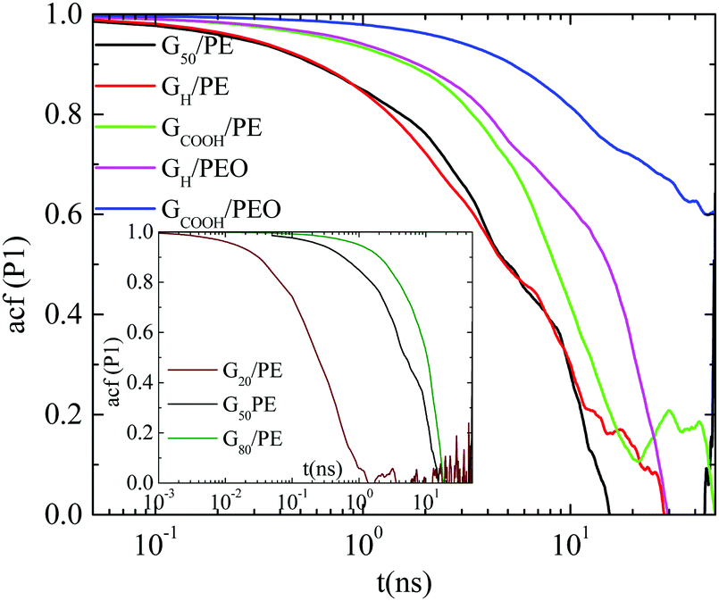Fig. 3 Time autocorrelation functions of P₁(t) for all the systems at T = 450 K.

The orientational dynamics of the nanographene sheets can be further quantified by defining a characteristic relaxation time for the half-diagonal vector, as the time integral of the P₁(t) curves shown above. To achieve this, P₁(t) data presented above are fitted with a KWW function , where A is a pre-exponential factor, which takes into account relaxation processes for very short times, τ_KWW is the relaxation time and β is the stretch exponent, which takes into account the deviation from the ideal Debye behavior. Then a characteristic orientational relaxation time is defined as the time integral of P₁(t): 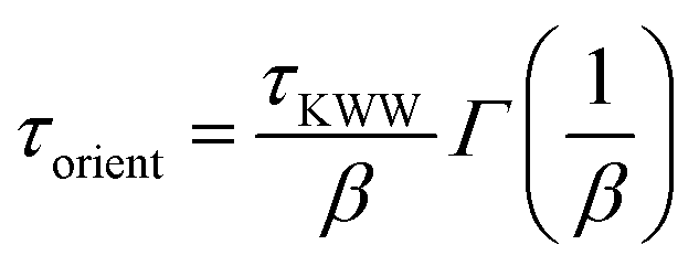. Note here that fitting of these curves is restricted to times up to about ∼10–20 ns, beyond which data become rather noisy, especially for the systems of PEO nanocomposites. Results for the orientational relaxation time (τ_orient) and the exponent β are presented in Table 2. In the PEO matrix the hydrogenated graphene is ∼2.5 times slower than that in the PE matrix, while the carboxylated sheet is ∼4 times slower in PEO compared to PE. Moreover, the carboxylated flakes are slower than the hydrogenated ones ∼1.5 times in the PE matrix and ∼2 times in the PEO matrix. β-values show a rather narrow distribution of relaxation times for all the systems, as β is in the range 0.8–1 in all cases. The size dependence of the orientational dynamics is presented in the inset of Fig. 3 and has been analyzed in our previous work.³¹ As in the case of the translational dynamics, decorrelation is faster for the smaller sheets.

A similar comparison in the orientational motion of the functionalized graphene flake between the G_H/PE (80mer) and G_H/PEO systems has been performed and the corresponding results for τ_orient are presented in Table 2. Again the motion of the hydrogenated sheet in PE 80mer exhibits similar orientational dynamics to that of PEO.

(B) Dynamics in the body frame – anisotropic Brownian motion

Since a nanographene sheet is a non-spherical object, its diffusion in a medium is expected to be anisotropic with respect to its plane, at least for short times. In order to investigate this, we analyze graphene's motion in the body frame. Note that theoretically (rigid) graphene sheets (i.e., flat frozen flakes) are very closely described by perfectly oblate ellipsoids. However, the morphological transitions (rippling) of the flakes in the nanocomposites induce changes in their shape. Such conformational transitions can also potentially affect the anisotropic diffusion, enhancing or suppressing the difference between the different components of the Brownian motion. This is exactly the issue that we address in the following, highlighting the differences between the diffusion of graphene flakes and perfectly oblate ellipsoids.

Translational dynamics. First, the translational dynamics is examined by calculating the different components of graphene center-of-mass MSDs: (a) normal to the major axis, (ΔR²)_X′Y′, and (b) parallel to the major axis, (ΔR²)_Z′, following the procedure described in the Analysis of Model Configurations section (see Fig. 1c). For the motion normal to the major axis the average of X′ and Y′ components is calculated.

Results for the MSD components of nanographene (pristine and functionalized) sheets in the PE and PEO matrices are presented in Fig. 4a and b. The anisotropic character of nanographene's Brownian motion is apparent in all the systems: there is a clear difference between the two components of MSD for short times (i.e., the subdiffusive regime), which, as expected, is eliminated for longer times, since the diffusion of the sheet in the long time regime becomes isotropic (i.e., linear regime). The motion normal to the major axis (X′Y′ component of MSD) is faster compared to the one parallel to the major axis (Z′ component). Furthermore, from the data shown in Fig. 4 it is clear that (a) for short times the difference between the X′Y′ and Z′ components of the mean squared displacement is higher for pristine graphene compared to the carboxylated one in the same matrix (PE) (Fig. 4a); (b) by comparing the two different matrices, a slightly smaller difference between the two components exists in the case of PEO, which underlines the effect of polymer–graphene interactions (Fig. 4b); and (c) in all cases the difference is gradually reduced and beyond a certain time, about ∼[20–30] ns, the diffusion becomes isotropic (i.e., linear regime – Fickian diffusion). The systems with hydrogenated graphene behave very similarly to the ones with pristine graphene.

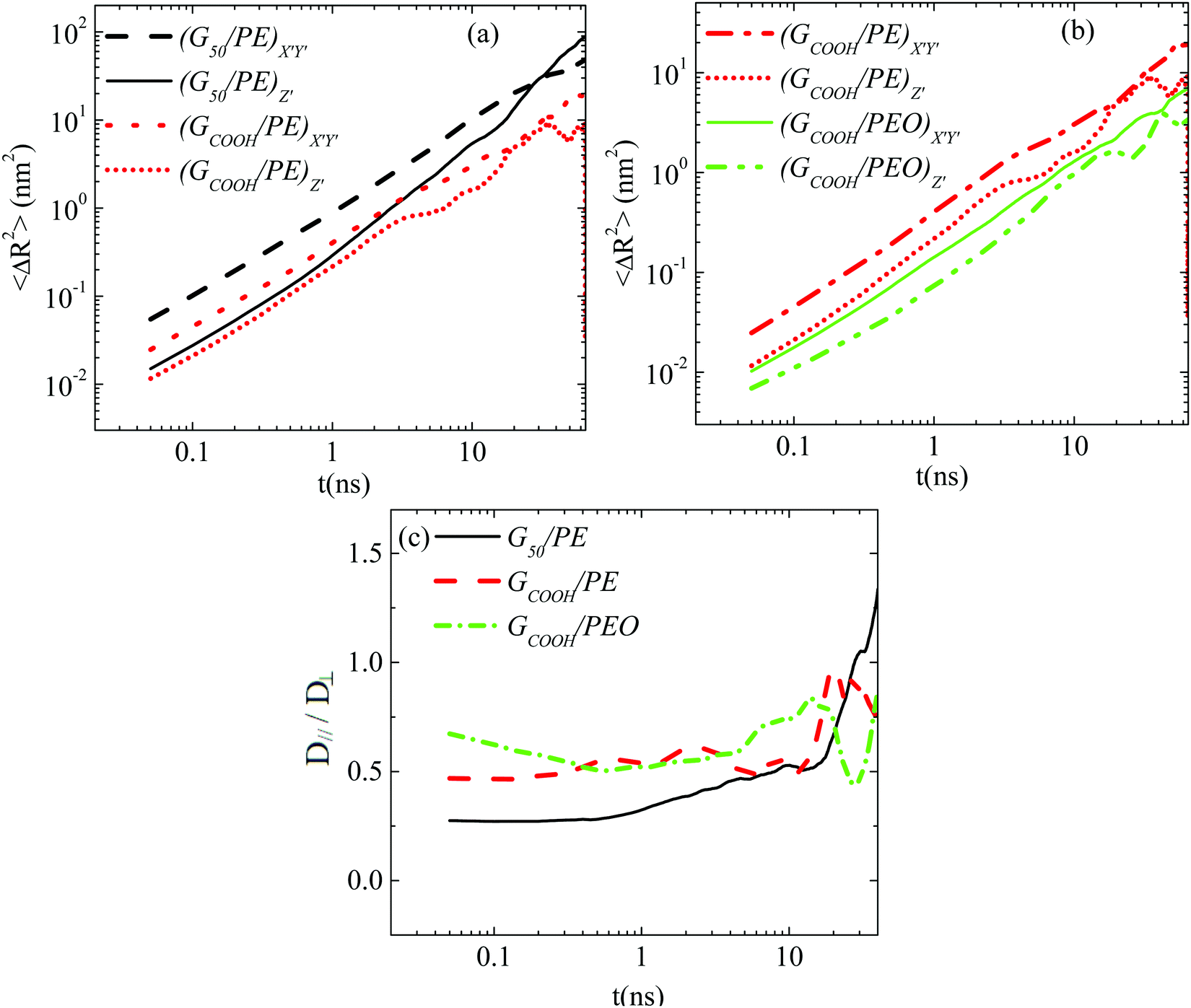Fig. 4 The graphene's MSD X′Y′ and Z′ components, defined on the body frame, as a function of time for the (a) G₅₀/PE and G_COOH/PE systems and (b) G_COOH/PE and G_COOH/PEO systems. (c) The D_‖(t)/D_⊥(t) ratio as a function of time for the G₅₀/PE, G_COOH/PE and G_COOH/PEO systems.

Then we have calculated effective diffusion coefficients for graphene flakes, defined as 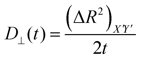and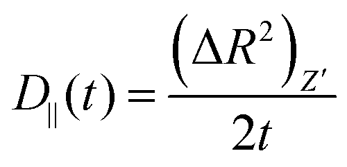 and their D_‖(t)/D_⊥(t) ratio as a function of time is presented in Fig. 4c for the G₅₀/PE, G_COOH/PE and G_COOH/PEO systems. D_‖(t)/D_⊥(t) attains the lowest value ∼0.26 for pristine graphene, but comparable values ∼0.5–0.6 for carboxylated graphene in the two polymer matrices, for short times. The difference between the two diffusion coefficients is bigger in the case of pristine graphene, where the two components of MSD have the highest deviation (Fig. 4a). Conformational transitions of the graphene flakes can be thought of as a possible reason for this observation. Indeed, we have observed bigger ripples in the pristine nanographene compared to the functionalized sheets, which result in bigger deviations from the ideal shape (i.e., oblate ellipsoid). Functionalization of graphene is an important factor which suppresses the rippling; therefore, it affects the dynamics. Representative results concerning the amplitudes of the ripples are presented in Table SI-3 (ESI†). Moreover, carboxyls are bulky groups, added to the edges, which are lying out-of-plane, hindering the in-plane motion. Therefore, they constitute an additional reason for the suppression of the anisotropy in the carboxylated graphene flakes. The D_‖(t)/D_⊥(t) ratio approaches one only in the limit of long times when the two components of the MSD almost coincide and the diffusion becomes isotropic. Moreover, the above calculations are in qualitative agreement with the predictions based on eqn (1)–(3) for oblate ellipsoids, since the D_‖(t)/D_⊥(t) ratio for nanographene sheets of (50 × 50) Ų area is <1, in a range of [0.26–0.7], for the different systems. Values are constant for short times, when orientational decorrelation of the sheets has not been achieved yet, whereas they reach 1 later on. The value predicted from eqn (1)–(3) for a perfectly oblate ellipsoid of (50 × 50) Ų area is 0.7 in good agreement with our calculations.

Orientational dynamics. In the following we examine the anisotropic dynamics with respect to the rotational motion of the flake. Our calculations are based on the autocorrelation function of 〈cos θ(t)〉 for the three angles (θ₁, θ₂, θ₃) which are described in Fig. 1b. Fig. 5a presents data for the G₅₀/PE system where anisotropy among the three components of the orientational motion is clear. Rotational diffusion around the Z′ axis, which corresponds to θ₁ and θ₂ angles (we call these X′ and Y′-components), is faster than the diffusion around the X′ and/or Y′ axes, which corresponds to the θ₃ angle (we call this Z′-component). Moreover, the X′ and Y′ components are, as expected, equivalent and we present their average as X′Y′. It is interesting to observe that the Z′-component diverges from X′Y′ for times up to ∼20 ns, beyond which the curves tend to overlap. This time scale is very similar to the one at which anisotropy disappears in the translational diffusion.

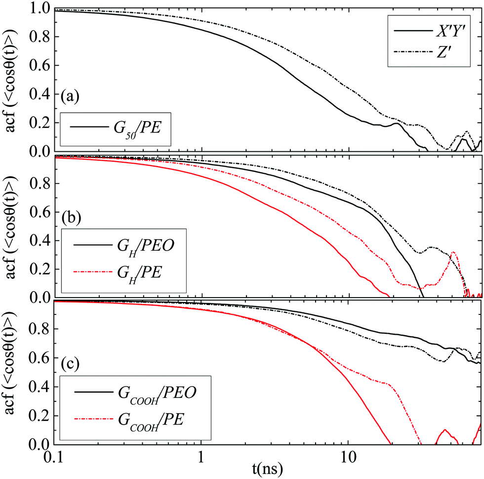Fig. 5 Time autocorrelation functions of 〈cos θ(t)〉 for the direction cosines (X′Y′ and Z′ – rotation) of the (a) G₅₀/PE, (b) G_H/PEO and G_H/PE systems and (c) G_COOH/PEO and G_COOH/PE systems.

Similar to pristine graphene is the behavior of the hydrogenated sheet in the PE matrix, whereas in the PEO matrix the difference between the two components is less pronounced (Fig. 5b). In Fig. 5c results for the carboxylated sheet in the two matrices are presented. For the G_COOH/PEO system autocorrelation functions attain still high values for the time window of the current simulation; therefore, we cannot extract any conclusion for their anisotropy. For the G_COOH/PE system the two components are identical for short times up to ∼10 ns, in the following the X′Y′ component is faster up to ∼30 ns before data become noisy.

Overall, interactions between the graphene flake and the matrix seem to be crucial for both the translational and orientational motions of the sheet. The stronger the interactions the lower the induced anisotropy, which is highlighted in the PEO nanocomposites. Furthermore important is the role of the end functional groups which also suppress anisotropy. Anisotropic diffusion can induce anisotropy in the overall properties of the nanocomposite, which in some cases is important to be controlled or at least understood.

Temperature effect (COOH/PEO). Next, we examine the effect of temperature on the dynamics of the graphene sheets. The presented results concern a range of temperatures T = [318, 340, 370, 400, 450] K for the carboxylated sheet in the PEO matrix. As expected, as the temperature decreases, both the translational and orientational dynamics of the graphene sheets become slower.
Lab frame. A comparison of the translational motion among the systems at different temperatures is depicted in Fig. 6a ((G_COOH/PEO)_318–450 systems), where the time dependent effective diffusion coefficients, derived from the mean squared displacements, are presented.

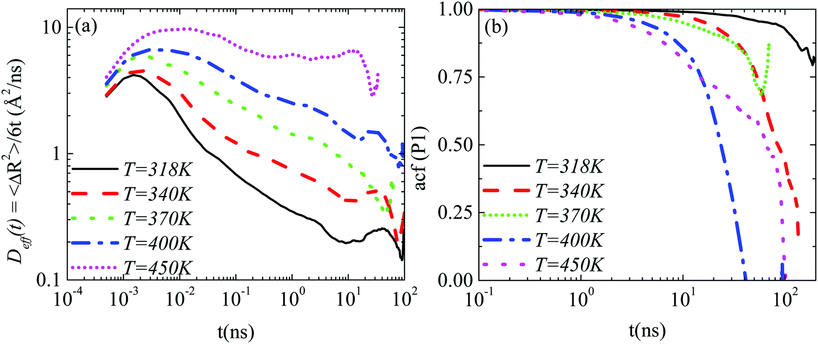Fig. 6 (a) The effective diffusion coefficient (D_eff(t)) of the center of mass of the graphene flake as a function of time for nanocomposites with carboxylated graphene sheets in PEO ((G_COOH/PEO)_318–450 systems) at various temperatures. (b) Time autocorrelation functions of P₁(t) for the half diagonal vector of the graphene sheet for the (G_COOH/PEO)_318–450 systems.

The retardation of the translational dynamics at lower temperatures is obvious. On top of that it is interesting to observe that, in the time window of the simulations, the motion of the graphene flake is not diffusive in the PEO matrix at any temperature, but the highest one (450 K), where a plateau in D_eff(t) is observed. A decrease in temperature leads to a broadening of the non-linear, subdiffusive regime of the BM of the nanographene sheet in a polymer matrix.

An analogous comparison among the different temperatures is performed for the orientational motion, through the calculation of the autocorrelation function of the first Legendre polynomial, P₁(t), for the half diagonal vector of the graphene sheet (Fig. 1b). Results, which are presented in Fig. 6b, illustrate the retardation of the orientational motion with temperature as well. Characteristic times for the decorrelation of the vector are extracted from fits with KWW functions and are discussed below. Note here that at the lowest temperature value (318 K) the decorrelation of the half diagonal vector ACF of the sheet is limited in the time window of the simulation; thus the characteristic time that we have extracted from the KWW fit is used as a rough estimation of the slowdown of the graphene dynamics with decreasing temperature. For this reason a different (star) symbol is used in the corresponding graph (Fig. 8a).

Body frame. The way that the anisotropy in diffusion is affected by the temperature is presented in Fig. 7. A comparison of the parallel and perpendicular MSDs to the major axis at three temperatures is performed for the G_COOH/PEO system. Clear differences between the two components, mainly in the short time regime, are observed, for all the temperatures studied here. No particular temperature effect is detected, rather than a small suppression of the difference between the two components of the MSD at lower temperatures.

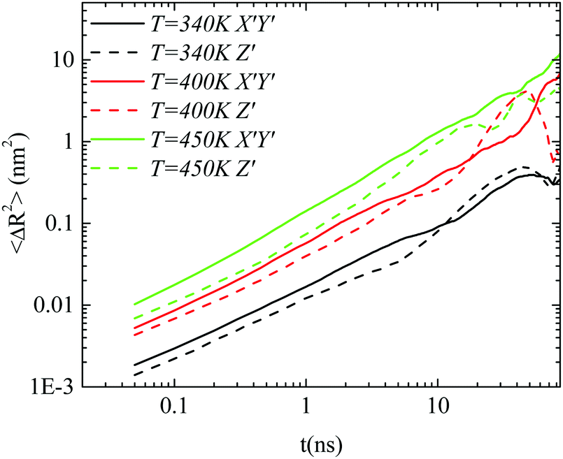Fig. 7 The X′Y′ and Z′ components, defined on the body frame, of the mean squared displacement as a function of time for the G_COOH/PEO system at three different temperatures.

Polymer–graphene coupling. In the following we examine whether the motion of the nanographene flake is coupled with the motion of the polymer amount which is adsorbed on its surface. For this reason, the characteristic decorrelation times which correspond to Fig. 6b are presented in Fig. 8a, as a function of temperature, together with the terminal relaxation times of PEO chains (i.e., relaxation time of the end-to-end vector) in the first adsorption layer (1.5 nm from the surface) and in the bulk regime (5.0 nm from the surface).

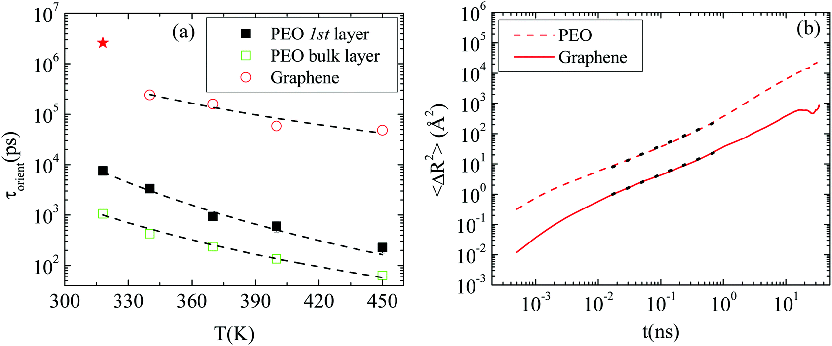Fig. 8 (a) Terminal relaxation times for PEO in the first adsorption layer and in the bulk together with relaxation times for the half diagonal vector of graphene as a function of temperature for (G_COOH/PEO)_318–450 systems. Dashed lines correspond to fits with exponential functions. (b) The mean squared displacement of the center of mass of the polymer chains in the first adsorption layer (solid lines) together with the mean squared displacement of the center of mass of the nanographene sheet (dashed lines) as a function of time for the G_COOH/PEO system at T = 450 K.

Fits with an exponential function of the Arrhenius form (t = A exp(−B/T)) are performed (dashed lines). For the polymer chains the decay of the relaxation time with temperature provides an exponent B equal to −4076.9 K for chains in the vicinity of the graphene layer, and −3092.8 K in the bulk. Similarly, an exponential decay is observed for the decorrelation time of the nanographene flake with temperature, which indicates a coupling in the orientational motion of the polymer and nanographene. The exponential fit in the case of nanographene was made on the last four points and an exponent almost two thirds of the one stands for the polymer, very close to the surface, was extracted (B = −2452.1 K). An estimation of activation energies can be extracted from these fits, resulting in E_{act_polymer_1st layer} = −33.9 kJ K⁻¹ mol⁻¹, E_{act_polymer_bulk} = −25.7 kJ K⁻¹ mol⁻¹ and E_{act_graphene} = −20.4 kJ K⁻¹ mol⁻¹. This shows that the effect of the temperature is stronger on the polymer chains (i.e., ∼1.5 times faster decorrelation of the orientation of the chains in the first adsorption layer, with temperature, compared to the nanographene flake). The activation energies of the polymer in the bulk regime and nanographene are comparable, with the latter still being a bit higher. Thus polymer relaxation is more sensitive to the temperature change at any distance from the surface compared to the nanographene flake.

On top of that, the mean squared displacement of the center of mass of the polymer chains, which lie on the graphene surface (i.e., the first adsorption layer of 1.5 nm width), is calculated and compared to the mean squared displacement of the center of mass of the nanographene sheet (lab frame). To quantitatively study the different dynamical behavior of polymer chains around nanographene, the area around the sheet is divided into two regions (one parallel to the surface and one edge region) and the dynamics is calculated independently for the different regions.⁴⁷ Results for the G_COOH/PEO system at T = 450 K are presented in Fig. 8b, where dashed lines indicate the polymer's motion parallel to the nanographene sheet region and solid lines for nanographene's motion. Both curves are fitted with a power law function, for the same time period, which can be assigned to the sub-diffusive regime (dotted lines). A similar slope (0.85 for graphene; 0.9 for the polymer) of the MSD curves is observed for both components, which indicates a coupling in their translational diffusion too. For longer times the diffusive regime is observed for both components (i.e., slope ∼1). For very short distances from the nanographene, the polymer is strongly adsorbed on the surface of the nanographene flake; therefore its motion is affected by the motion of the sheet.

5. Conclusions

In the current work we have studied the dynamical behavior of nanographene sheets in polymer–graphene nanocomposites through atomistic molecular dynamics simulations. The Brownian dynamics of the nanographene sheets is explored in both the lab and body frames of the flake and valuable information is revealed for the motion of nanographene in the polymer matrix and the factors which can affect it.

Calculations in the lab frame provide the following results: translational dynamics are similar for pristine and hydrogenated nanographene in PE matrices. In PE nanocomposites nanographene diffuses more rapidly than that in PEO ones. This result is attributed to stronger polymer–graphene interactions, but in addition both the higher zero-shear viscosity of PEO compared to PE and the difference in their T_g values are determinant factors. The effect of the carboxyl edge groups is strong, since the carboxylated graphene sheets move more slowly than both the pristine and hydrogenated ones in both matrices. This highlights the effect of the electrostatic and possible H-bond interactions (for the PEO matrix) between the polymer and the functionalized nanographene sheet. On top of that, the mass difference between the pristine and functionalized nanographene flakes affects their dynamics correspondingly. Similar factors govern orientational dynamics. Correlations among the factors that determine the dynamics of the different nanocomposite systems provide important piece of information which can be transferred to systems with macroscopic graphene as well.

Since graphene is a two dimensional material, theory predicts inhomogeneity in its Brownian motion in terms of anisotropy between two directions, the in-plane motion (X′Y′) and the out-of-plane motion (Z′). However, theoretical relations are valid only for perfect shapes, like oblate or prolate ellipsoids, where constant diffusion coefficients are derived from the solution of the Navier–Stokes hydrodynamic equations. Diffusion is anisotropic for short times, while it turns into isotropic in the very long time limit, and for oblate ellipsoids the motion perpendicular to the major axis is faster than the one parallel to the major axis. According to a shape analysis procedure, unperturbed graphene sheets are closely described by oblate ellipsoids (thin discs) (see the ESI†). However, rippling of graphene, which is extensively affected by the interactions with the polymer matrix, induces changes in the shape of the sheets. These changes have a strong effect on the dynamics of the flake. Analysis of dynamics in the body frame reveals anisotropy between the two directions of motion (parallel and perpendicular to the major axis), with the motion perpendicular to the major axis being always faster than the one parallel to the major axis. Differences are more pronounced for pristine graphene. The effect of functional edge groups results in suppression of the differences between the two components of motion. Anisotropy is observed for times ∼20–30 ns beyond which the diffusion becomes isotropic (linear regime). Similar observations concerning the anisotropy stand for the rotational motion as well.

The temperature effect has been studied through the analysis of the autocorrelation function of the first Legendre polynomial for the half diagonal vector of graphene, which provides an effective activation energy. An analogous calculation for PEO very close to the surface (1st adsorption layer), based on the terminal relaxation times (i.e., end-to-end vector), shows that the decorrelation of the polymer orientation with temperature is ∼1.5 times faster than that of the nanographene. For both the polymer and nanographene, orientational relaxation times follow an exponential decay. In addition, in the translational motion, the mean squared displacements of the centers of mass of the polymer and nanographene versus time attain similar slopes. These observations indicate a coupling in the motion between the nanographene sheet and the amount of polymer very close to it.

In whole, interactions between the nanographene flake and the matrix have a strong effect on both the translational and orientational motion of the sheet. The stronger the interactions the lower the induced anisotropy. Proper functionalization of the graphene flakes specifies polymer–graphene interactions but determines the conformational transitions of the flakes as well; therefore, it could be used as potential control of the Brownian motion of the sheets.

Conflicts of interest

The authors declare no conflicts of interests.

Acknowledgements

A. N. Rissanou acknowledges the Crete Center for Quantum Complexity and Nanotechnology (CCQCN), Department of Physics, University of Crete, Heraklion, Crete, Greece, for financial support during the execution of this research. The research leading to these results has been co-funded by the European Commission under H2020 Research Infrastructures contract no. 695121 (project VI-SEEM).

References

1. A. Einstein, Ann. Phys., 1905, 322(8), 549–560.
2. A. Einstein, Ann. Phys., 2005, 14(S1), 229–247.
3. W. T. Coffey, Yu. P. Kalmykov and J. T. Waldron, The Langevin Equation: With Applications to Stochastic Problems in Physics, Chemistry and Electrical Engineering, World Scientific Series in Contemporary Chemical Physics, World Scientific Publishing Company, Singapore City, 2nd edn, 2004, vol. 14.
4. S. R. Aragón and R. Pecora, J. Chem. Phys., 1977, 66(6), 2506–2516.
5. N. Gerhard, J. Phys.: Condens. Matter, 2003, 15(1), S407.
6. D. M. Heyes, M. J. Nuevo, J. J. Morales and A. C. Branka, J. Phys.: Condens. Matter, 1998, 10, 10159–10178.
7. G. H. Koenderink, H. Zhang, D. G. L. Aarts, M. P. Lettinga, A. P. Philipse and G. Nägele, Faraday Discuss., 2003, 123, 335–354.
8. J. Kanetakis and H. Sillescu, Chem. Phys. Lett., 1996, 252(1–2), 127–134.
9. S. Martin, M. Reichert, H. Stark and T. Gisler, Phys. Rev. Lett., 2006, 97(24), 248301.
10. A. Pralle, M. Prummer, E. L. Florin, E. H. K. Stelzer and J. K. H. Hörber, Microsc. Res. Tech., 1999, 44(5), 378–386.
11. K. S. Novoselov, A. K. Geim, S. V. Morozov, D. Jiang, Y. Zhang, S. V. Dubonos, I. V. Grigorieva and A. A. Firsov, Science, 2004, 306(5696), 666–669.
12. A. A. Balandin, S. Ghosh, W. Bao, I. Calizo, D. Teweldebrhan, F. Miao and C. N. Lau, Nano Lett., 2008, 8(3), 902–907.
13. S. Latil and L. Henrard, Phys. Rev. Lett., 2006, 97(3), 036803.
14. C. N. R. Rao, A. K. Sood, K. S. Subrahmanyam and A. Govindaraj, Angew. Chem., Int. Ed., 2009, 48(42), 7752–7777.
15. K. Zhang, L. L. Zhang, X. S. Zhao and J. Wu, Chem. Mater., 2010, 22(4), 1392–1401.
16. L. Feng and Z. Liu, Nanomedicine, 2011, 6(2), 317–324.
17. S. Guo and S. Dong, Chem. Soc. Rev., 2011, 40(5), 2644–2672.
18. H. Jiang, Small, 2011, 7(17), 2413–2427.
19. K. P. Loh, Q. Bao, G. Eda and M. Chhowalla, Nat. Chem., 2010, 2(12), 1015–1024.
20. Y. Wang, Z. Li, J. Wang, J. Li and Y. Lin, Trends Biotechnol., 2011, 29(5), 205–212.
21. K. Karatasos, Macromolecules, 2014, 47(24), 8833–8845.
22. H. Kim, A. A. Abdala and C. W. Macosko, Macromolecules, 2010, 43(16), 6515–6530.
23. J. R. Potts, D. R. Dreyer, C. W. Bielawski and R. S. Ruoff, Polymer, 2011, 52(1), 5–25.
24. T. Ramanathan, A. A. Abdala, S. Stankovich, D. A. Dikin, M. Herrera Alonso, R. D. Piner, D. H. Adamson, H. C. Schniepp, X. Chen, R. S. Ruoff, S. T. Nguyen, I. A. Aksay, R. K. Prud'Homme and L. C. Brinson, Nat. Nanotechnol., 2008, 3(6), 327–331.
25. E. N. Skountzos, A. Anastassiou, V. G. Mavrantzas and D. N. Theodorou, Macromolecules, 2014, 47(22), 8072–8088.
26. S. Deng and V. Berry, Mater. Today, 2016, 19(4), 197–212.
27. Z. Li, I. A. Kinloch, R. J. Young, K. S. Novoselov, G. Anagnostopoulos, J. Parthenios, C. Galiotis, K. Papagelis, C.-Y. Lu and L. Britnell, ACS Nano, 2015, 9(4), 3917–3925.
28. L. Cui, X. Du, G. Wei and Y. Feng, J. Phys. Chem. C, 2016, 120(41), 23807–23812.
29. E. Jomehzadeh and N. M. Pugno, Composites, Part B, 2015, 83, 194–202.
30. F. Schedin, A. K. Geim, S. V. Morozov, E. W. Hill, P. Blake, M. I. Katsnelson and K. S. Novoselov, Nat. Mater., 2007, 6(9), 652–655.
31. A. Rissanou, A. Power and V. Harmandaris, Polymers, 2015, 7(3), 390.
32. A. N. Rissanou and V. Harmandaris, Soft Matter, 2014, 10(16), 2876–2888.
33. F. Guinea, B. Horovitz and P. Le Doussal, Solid State Commun., 2009, 149(27–28), 1140–1143.
34. M. Ma, G. Tocci, A. Michaelides and G. Aeppli, Nat. Mater., 2016, 15(1), 66–71.
35. F. Banhart, J. Kotakoski and A. V. Krasheninnikov, ACS Nano, 2011, 5(1), 26–41.
36. L.-H. Cai, S. Panyukov and M. Rubinstein, Macromolecules, 2011, 44(19), 7853–7863.
37. T. Ge, G. S. Grest and M. Rubinstein, Phys. Rev. Lett., 2018, 120(5), 057801.
38. O. M. Maragó, F. Bonaccorso, R. Saija, G. Privitera, P. G. Gucciardi, M. A. Iatì, G. Calogero, P. H. Jones, F. Borghese, P. Denti, V. Nicolosi and A. C. Ferrari, ACS Nano, 2010, 4(12), 7515–7523.
39. Y. Han, A. M. Alsayed, M. Nobili, J. Zhang, T. C. Lubensky and A. G. Yodh, Science, 2006, 314(5799), 626–630.
40. R. Vasanthi, S. Ravichandran and B. Bagchi, J. Chem. Phys., 2001, 114(18), 7989–7992.
41. R. Vasanthi, S. Bhattacharyya and B. Bagchi, J. Chem. Phys., 2002, 116(3), 1092–1096.
42. H. Shimizu, J. Chem. Phys., 1962, 37(4), 765–778.
43. W. Gao, L. B. Alemany, L. Ci and P. M. Ajayan, Nat. Chem., 2009, 1(5), 403–408.
44. J. Du and H.-M. Cheng, Macromol. Chem. Phys., 2012, 213(10–11), 1060–1077.
45. M. G. Martin and J. I. Siepmann, J. Phys. Chem. B, 1998, 102(14), 2569–2577.
46. J. Fischer, D. Paschek, A. Geiger and G. Sadowski, J. Phys. Chem. B, 2008, 112(8), 2388–2398.
47. P. Bačová, A. N. Rissanou and V. Harmandaris, Macromolecules, 2015, 48(24), 9024–9038.
48. J. Ramos, J. F. Vega and J. Martínez-Salazar, Macromolecules, 2015, 48(14), 5016–5027.
49. J. H. Walther, R. Jaffe, T. Halicioglu and P. Koumoutsakos, J. Phys. Chem. B, 2001, 105(41), 9980–9987.
50. Y. N. Pandey, A. Brayton, C. Burkhart, G. J. Papakonstantopoulos and M. Doxastakis, J. Chem. Phys., 2014, 140(5), 054908.
51. W. L. Jorgensen, D. S. Maxwell and J. Tirado-Rives, J. Am. Chem. Soc., 1996, 118(45), 11225–11236.
52. B. Hess, H. Bekker, H. J. C. Berendsen and J. G. E. M. Fraaije, J. Comput. Chem., 1997, 18(12), 1463–1472.
53. G. Bussi, D. Donadio and M. Parrinello, J. Chem. Phys., 2007, 126(1), 014101.
54. D. J. Evans and B. L. Holian, J. Chem. Phys., 1985, 83(8), 4069–4074.
55. A. A. Miller, J. Polym. Sci., Part A-2, 1968, 6(1), 249–257.
56. L. Hamon, Y. Grohens, A. Soldera and Y. Holl, Polymer, 2001, 42(24), 9697–9703.

---

Footnote

† Electronic supplementary information (ESI) available. See DOI: 10.1039/c9cp02074h

---