Laboratory EXAFS determined structure of the stable complexes in the ternary Ni(II)–EDTA–CN⁻ system

Abstract

Aqueous solutions of the ternary system Ni(II)–EDTA–CN⁻ are investigated with X-ray Absorption Spectroscopy (XAS) as a function of cyanide concentration with an enhanced laboratory von Hámos X-ray spectrometer. The near-edge structure of the spectra identifies unambiguously the formation of the pentacyanidonickel(II) complex at excess CN⁻ concentrations. An analysis of the extended energy range of the XAS spectra reveals the molecular structure of the distinct molecular components present and provides a detailed description of the barely detectable mixed ligand [NiEDTA(CN)]³⁻ complex. This thorough Extended X-ray Absorption Fine Structure (EXAFS) study demonstrates the potential of the emerging laboratory XAS spectrometers to become routine probes in various areas of chemistry, materials science, physics and related disciplines.

---

1 Introduction

X-ray Absorption Structure (XAS) spectroscopy is one of the most revealing experimental tools with which to acquire element selective information on the local electronic-, spin- and structural states of atoms in a wide range of materials including catalysts, fuel cell components, IT-related novel materials, biological systems, etc. (see e.g.ref. 1 and references therein). However, the high demand to use these techniques greatly exceeds the instrumental availability: XAS methods are performed at synchrotrons, which are exceedingly overbooked and require a very long waiting period for measurements. Therefore, XAS analysis is hardly accessible to the wider scientific community, which would profit from routine X-ray spectroscopic measurements.

In recent years, however, attempts have been made to adapt state-of-the-art detector and analyser technologies to standard laboratory X-ray sources with the aim to build tabletop high energy resolution spectrometers.^2–8 While these spectrometers cannot compete with the brilliance of large scale facilities, they proved to be quite applicable to routine X-ray Absorption Near Edge Structure (XANES)^2,8,9 or X-ray emission spectroscopic^5,7,8 investigations on condensed samples. These promising first results encourage us to widen the field of laboratory spectroscopies to include one of the most used X-ray techniques: Extended X-ray Absorption Fine Structure (EXAFS).^1,10 EXAFS became a most fruitful method to describe molecular structure, providing atomic distances with the precision of an X-ray diffraction measurement but with the advantage of being an element selective local technique which is suitable for investigating non-crystalline samples including liquids. These properties make it an ideal laboratory characterization tool for researchers in chemistry, physics, environmental sciences, etc. and even for industrial applications. The demand for such a laboratory tool is indeed high and urgent: a first validation of laboratory EXAFS on nickel foil with a Johann-type spectrometer has just been published by Jahrman et al.⁸

The present work on a ternary Ni–EDTA–CN⁻ solution series demonstrates that a thorough EXAFS study can indeed be performed with a laboratory X-ray source. The variation of the complex equilibria with the cyanide concentration was studied previously via laboratory XANES,⁹ and the results revealed the speciation of the Ni. However, the structure of the complexes could not be determined in the energy range available in a single spectrometer geometry. Also, the pure XANES signal from two intermediate complexes was not obtained with good enough accuracy. Now the system has been revisited using an improved laboratory spectrometer; two more concentration points were added, and the structural parameters of the species occurring in solution were evaluated. In particular, at moderate cyanide concentrations (0 ≤ c_CN/c_Ni ≤ 4) the structure of the intermediate complex was determined to have a 1 : 1 EDTA : CN⁻ ligand ratio, where the in-bonding cyanide ligand displaces an EDTA oxygen donor atom from the nickel. Moreover, it is shown unambiguously that by increasing the cyanide ion concentration in the solution above a 4 : 1 ratio (which occurs at c_CN = 1.0 M in our case) between the cyanide and the nickel cations, a pentacoordinated nickel cyanide compound starts to form alongside the co-existing tetracyanidonickel(II). Complemented with evaluated laboratory EXAFS spectra of some reference samples, this paper demonstrates clearly that by exploiting novel detectors and analysers, a reasonable fraction of common EXAFS experiments can be performed without the need to apply for synchrotron beamtime. As concentrated cyanide solutions are very poisonous, the local laboratory venue is better suited for this experiment from a safety point of view, since it allows us to eliminate the dangers that can occur during long distance transport of such materials, as well as accidental human exposure in the busy sample preparation laboratories and beamlines of large scale facilities. Working in the familiar environment of the home institution makes enforcing the necessary safety measures easier, and decreases the associated dangers.

2 Experimental

2.1 Sample preparation

Transmission optimized Ni metal foil from EXAFS Materials (http://exafsmaterials.com/) and concentrated (4.3153 mol%) aqueous NiSO₄ solution were used for reference spectra. Preparation of the Ni–EDTA–CN solutions is described in ref. 9, with two extra concentration points added in this work. The 9 aqueous solutions contain 0.25 M Ni²⁺ cations, 0.30 M EDTA (ethylenediaminetetraacetic acid) ligand and c_CN = 0, 0.15, 0.25, 0.35, 0.50, 0.75, 1.00, 2.00 and 3.00 M CN⁻ anions with the pH set to 11. All the liquid samples were measured in a custom made cell,⁹ with the sample thickness set to 0.5 mm and 1 mm for the NiSO₄ and Ni–EDTA–CN samples, respectively.

2.2 EXAFS data collection

X-ray absorption spectra were recorded with a slightly improved version of the laboratory high energy-resolution von Hámos hard X-ray spectrometer described in ref. 4. The X-ray source was set to 10 keV and 40 mA, and the detector to an 8 keV threshold. Although the Ni K-edge XANES region (about 8300–8400 eV) can be measured with a fixed geometry of the spectrometer's source, analyser crystal and detector, for the longer EXAFS region (ca. 8300–8900 eV) additional energy ranges at smaller Bragg-angles have to be recorded, and thus other geometries are also required to cover the desired range. We chose a data acquisition strategy where the mean Bragg angle was decreased step by step by shifting the detector by 4 pixels (200 μm) away from the source and the analyser by a corresponding 100 μm parallel with the detector, and rotating the spectrometer's platform below the X-ray tube to keep the source's direct beam on the analyser crystal. These steps were repeated 350 times (70 mm total shift for the detector) to scan the full Ni EXAFS spectrum. The 4 pixel shift is only 1/320 of the energy span at one detector position. So the whole 350 step cycle covers approximately 2× the energy span of the detector. The resulting spectra were averaged over the measuring time for each pixel for both the sample out (I₀) and for the sample in spectra. In order to improve the signal-to-noise ratio, in the case of the Ni–EDTA–CN solutions both the full 350 steps and the second half (175 steps) of the EXAFS scans were repeated to give adequate statistics. Raw EXAFS data were treated in exactly the same way as a standard synchrotron EXAFS spectrum is treated. Data analysis details are given in the corresponding parts of Section 3.

3 Results and discussion

3.1 Reference EXAFS spectra

In order to authenticate the laboratory EXAFS spectrometer's capabilities, spectra of Ni metal foil and a concentrated NiSO₄ solution were recorded (Fig. 1). The acquisition time necessary for such a full laboratory EXAFS spectrum with good statistics is on the order of a typical shift at a synchrotron (6–8 h), once an appropriate I₀ spectrum is available. As in the case of the previously reported XANES spectra,⁴ the energy resolution and spectral features agree perfectly with the equivalent synchrotron data. The k- and R-space plots show that the data quality is quite adequate for a proper analysis. For the Fourier-transform, data in the k-range of 3 Å⁻¹ to 13 Å⁻¹ or 12 Å⁻¹ (Ni metal or NiSO₄, respectively) were used, while the fit window was R = 1–6 Å. Due to the strong and poorly background-subtracted fluorescence lines coming from the X-ray tube, spectral points in the energy range of 8512–8546 eV as well as 8624–8666 eV are cut out from the Ni foil spectrum and between 8648 and 8663 eV from the NiSO₄ data. Note that these energies do not correspond to the real energy of the fluorescent X-rays, since they are coming through different harmonics of the crystal: the absorption is measured through the fourth harmonic of the Si(111) reflection, while the fluorescence reaches the detector through the third one. Unfortunately, the energy threshold of the detector is not sufficient to fully exclude these peaks. This cutting out was done with the deglitching tool of the Athena software of the Demeter software package,¹¹ and automatically compensated with the built-in interpolation routines through the energy-to-wavenumber conversion process. R-Space spectra were fitted with the Artemis program of the same package, the FEFF 6.01¹² calculations being based on cif files (9008476 and 1011189 for Ni metal and NiSO₄, respectively) taken from the Crystallography Open Database.¹³ The fits reproduced very well the literature data (Table 1). Geometry optimization with Density Functional Theory (DFT) calculations was also carried out for the [Ni(H₂O)₆]²⁺ complex using the ORCA 3.0¹⁴ software package with BP86^15,16 and B3LYP^17–19 functionals, the TZVP basis set,^20,21 and the COSMO solvation model parametrized for water solvent,²² similarly to that for the other measured complexes, detailed in ref. 9. The Ni–O bond lengths obtained with the BP86 and B3LYP functionals are 2.076 Å, and 2.088 Å, respectively, in agreement with the experimentally determined value.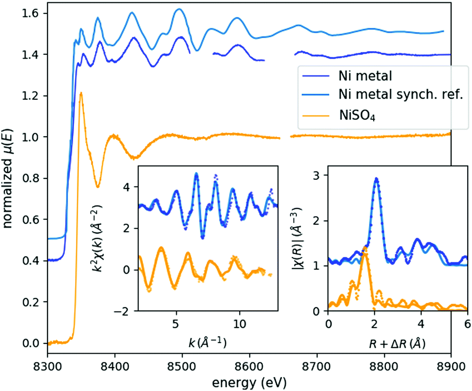

Fig. 1 EXAFS spectra of Ni metal foil (blue) and cc. NiSO₄ solution (orange). Respective sample acquisition times: 6.5 h and 9 h. Left and right insets show the corresponding k- and R-space spectra, respectively, where the experimental data is plotted with dots and the fit is shown with lines. A synchrotron reference EXAFS scan is also plotted in light blue above the laboratory Ni metal spectrum.⁸

Table 1 Fitted parameters of the reference EXAFS spectra

Parameter	Ni metal		cc. NiSO4
	Exp.	Ref.	Exp.	Ref.
Amplitude reduction factor	0.54(7)		0.51(4)
Edge energy (eV)	8332(1)	8333	8343(2)	8340.98^23
First neighbour distance (Å)	2.442(8)	2.492	2.07(2)	2.035
Debye–Waller factor (Å^2)	0.005(1)		0.004(1)

---

3.2 EXAFS spectra of the mixed Ni–EDTA–CN solutions

In aqueous solutions of nickel, EDTA and cyanide ions with different molar ratios, four different species of nickel could be observed: [NiEDTA]²⁻ and [Ni(CN)₄]²⁻ at the optimal compositions of Ni : EDTA : CN 1 : 1 : 0 and 1 : 1 : 4, respectively, as well as two additional compounds, [NiEDTA(CN)]³⁻ and [Ni(CN)₅]³⁻, forming in chemical equilibrium with these basic species at intermediate and high CN⁻ concentrations. The mole fraction of these molecular complexes depends on the relative concentrations of the constituents as shown in Fig. 2, which has been plotted based on data from ref. 9 and 24–26. As the spectral signals of the [NiEDTA(CN)]³⁻ and [Ni(CN)₅]³⁻ compounds are difficult to separate with conventional methods, the determination of their exact structure is very challenging. XAS methods, however, are most suitable to perform this task, even at laboratories.

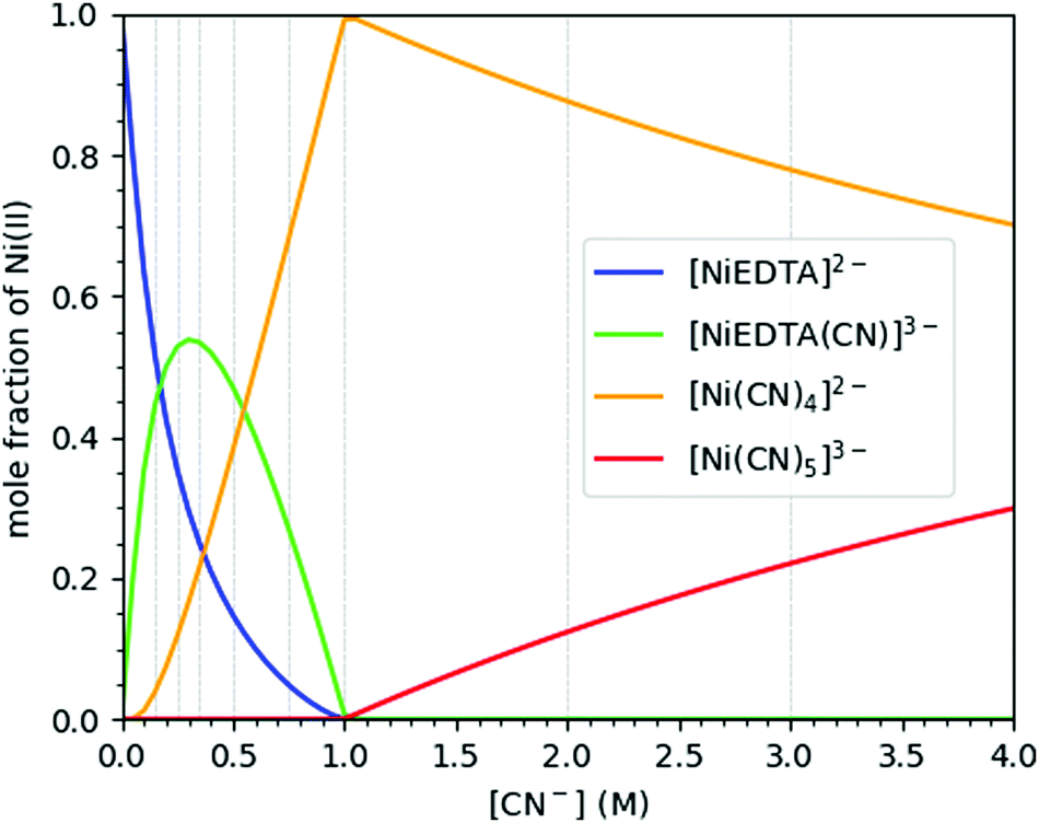Fig. 2 Molar distribution of the different nickel compounds in a Ni–EDTA–CN ternary solution as a function of cyanide concentration. The Ni²⁺ and EDTA concentrations are set to 0.25 and 0.3 M, respectively. The hereby used CN⁻ concentrations are indicated with vertical grey lines. Data re-plotted from ref. 9.

Fig. 3 shows the recorded EXAFS spectra for all samples of the studied ternary Ni–EDTA–CN⁻ system with cyanide concentrations between 0 and 3 M. Typical total data acquisition times for these 250 mM Ni²⁺ solutions were a full day, except the last sample with c_CN = 3 M, where a red layer precipitated on the sample holder's window in a few hours, making the transmission data unreliable. Thus, for this sample the measurement was repeated with a fresh sample (and a clean sample holder) three times with a total of 9 h of acquisition. Even with this strategy, it was not possible to reach good enough quality for EXAFS analysis, although the XANES part is satisfactory. This exemplifies well one of the limits of laboratory EXAFS experiments, arising due to their relatively long spectral acquisition times. However, we are in the process of developing appropriate flow cells to circumvent this obstacle.

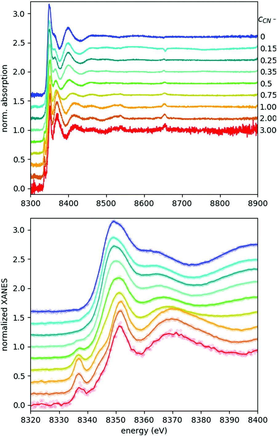Fig. 3 (top) Energy space Ni K-edge X-ray absorption of the Ni–EDTA–CN system with varying cyanide ion concentration (indicated in mols on the right side of the panel). (bottom) Zoom-in view of the XANES part of the absorption signal. Here, the lines show binned data with a bin size = 3, while raw data is plotted with faded dots. Each spectrum is normalized to 0 at low energy and 1 at high energy, and then offset for a visible comparison.

The XANES spectral features (the spectra are replotted in the bottom panel of Fig. 3, while some parameters are shown in Fig. 4) follow nicely those reported in ref. 9. Thanks to the higher data quality here, even the shift of the edge position can be clearly tracked, and it matches excellently the evolution of the pre-edge peak. As discussed in ref. 9, the pre-edge peak arises almost exclusively from the square planar [Ni(CN)₄]²⁻ component, making it a potent indicator of this species. Apparently the edge positions follow very closely the trend set by the pre-edge intensities, which suggests that the electronic changes reflected by the edge shift are most dominantly connected to the tetracyanidonickel(II) component, too. However, for further discussion of this feature as well as for evaluation of the EXAFS data the contributions of the unique species have to be separated.

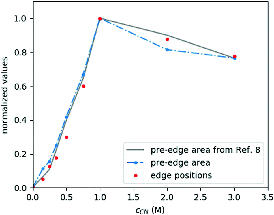Fig. 4 Spectral changes in XANES of the Ni–EDTA–CN system due to the evolution of the different species with c_CN. Parameters are normalized to the c_CN = 0 and 1 M samples, corresponding to the sole [NiEDTA]²⁻ and [Ni(CN)₄]²⁻ signals, reflecting the relative tetracyanidonickel content.

3.3 Separation of the occurring species

As the XAS spectra of all solutions are superpositions of those of the occurring species, a key step in evaluating the experimental data is to separate the individual contributions. The speciation data (highly correlated in the present case with the pre-edge area of the spectra, as described above, see Fig. 2 and 4) can be used to decompose the raw spectra to reconstruct the spectra of the pristine occurring species.

This is demonstrated in Fig. 5 for the most challenging case (due to precipitation, vide supra), where the XANES part of the spectrum of [Ni(CN)₄]³⁻ is shown. This spectrum has been reconstructed from the original data of solutions with c_CN = 2 M and 3 M, where the presence of this species is non-negligible. Based on the area of the pre-edge, the ratio between the [Ni(CN)₄]²⁻ and [Ni(CN)₅]³⁻ complexes was determined, and a respectively weighted tetracyanido-spectrum was subtracted from the solution's spectrum, the remaining signal being that of the pentacyanidonickel(II) complex. The XANES data of the sample with c_CN = 1 M (which is supposed to have almost exclusively the [Ni(CN)₄]²⁻ molecule) and the reconstructed data for the pentacyanido complex are then contrasted with the theoretically modelled spectra. The pre-edge region was modelled with time-dependent DFT (TD-DFT) calculations, while the full XANES spectra were calculated with FEFF (details of the calculations can be found in ref. 9, where a similar comparison has also been made; however, the improved data quality makes it worth reporting a new version of this figure). It is apparent in Fig. 5 that the experimental spectra follow nicely the calculated ones for both components, and their difference. Consequently, in addition to demonstrating the spectral separation method, these spectra also verify the formation of the pentacyanidonickel(II) complex at these high cyanide concentrations. The XAS spectrum of the pure [NiEDTA(CN)]³⁻ species was obtained similarly from the data with lower cyanide concentration (0 M < c_CN ≤ 0.5 M), where the [NiEDTA(CN)]³⁻ component has about a 50% mole fraction.

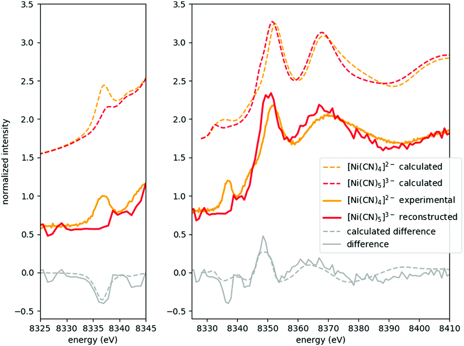Fig. 5 Calculated and experimental/reconstructed XANES spectra for the [Ni(CN)₄]²⁻/[Ni(CN)₅]³⁻ complexes, respectively. The left panel compares measured/reconstructed pre-edges with TD-DFT calculations, while the right panel shows the full experimental XANES spectra and the corresponding FEFF calculated ones. The reconstructed [Ni(CN)₅]³⁻ spectrum is binned with a bin size = 3.

The reconstructed spectra of the two species which do not occur solely (namely [NiEDTA(CN)]³⁻ and [Ni(CN₅)]³⁻) enable us to determine their absorption edge positions, as well. The main absorption edge of a 3d element stems from the excited electronic 1s–4p transition and it shifts in energy with the changes of the 3d valence electron orbital occupation due to its screening effect. Thus it is usually used to determine the oxidation state. Compared to the base [NiEDTA]²⁻ molecule, the [NiEDTA(CN)]³⁻ intermediate complex doesn't show any relevant variation in the edge position (both being at 8345.0 eV, derived from the maximum of the spectra's first derivative), while the homoleptic cyanido complexes, especially tetracyanidonickel(II), have considerably higher edge energies (8348.8 eV and 8347.0 eV for [Ni(CN₄)]²⁻ and [Ni(CN₅)]³⁻, respectively). This is in good accordance with the assumed shorter metal–ligand distances in the case of the cyanido complexes, which will be quantitatively analysed in the following section.

3.4 Structure determination

The solution structure of [NiEDTA]²⁻ and [Ni(CN)₄]²⁻ has long ago been determined with EXAFS at synchrotrons. Thus the laboratory data can be directly compared to those in the literature. The reduced, wave-number-transformed spectra of our data are compared to those measured at synchrotrons in the top and bottom panels of Fig. 6A (the synchrotron data are imported from ref. 27 and 28). While the data quality of the synchrotron recorded spectra is clearly superior, all features in the k-space spectra agree very well with those derived from the laboratory data.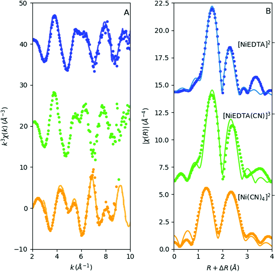

Fig. 6 k and R space EXAFS of the 2 basic species + the reconstructed intermediate complex. Left: Laboratory (dots) + synchrotron (lines) spectra, right: laboratory R space spectra (without phase correction, displayed with dots) with fits (grey lines).

In contrast to the reference Ni metal and NiSO₄ samples, the lower signal-to-noise ratio due to the lower nickel concentration in the Ni–EDTA–CN system hinders the use of data at high wave numbers. Hence the Fourier-transform window was k = 3–10 Å⁻¹. Still, the R-space EXAFS fits on both the first and second shell with an R window of 1–3 Å show good agreement with the DFT calculated structures for all three species (Fig. 6B). Amplitude reduction factors were set to 1, while the Debye–Waller factors vary between 0.003 and 0.006 Ų for the single scattering paths. Coordination numbers were fixed. E₀ values were fitted independently and were −2(1) eV, −2(1) eV and −4(2) eV for [NiEDTA]²⁻, [NiEDTA(CN)]³⁻ and [Ni(CN)₄]²⁻, respectively. The deviation of the atomic distances from the FEFF calculated values (ΔR) and the Debye–Waller factors (σ²) were fitted with one ΔR and one σ² parameter for the first shell Ni–O_EDTA and Ni–N_EDTA bonds, one pair of ΔR and σ² for the second shell Ni–C_EDTA bonds and two individual ΔR and σ² parameters for the Ni–C_CN and Ni–N_CN bonds. The resultant fitted bond lengths are summarized in Table 2. Multiple scattering paths with a FEFF calculated rank above 20 were included in the fits. Their path lengths were deduced from the parameters of the single scattering paths, while their Debye–Waller factors were approximated to be twice the corresponding single scattering path's σ².

Table 2 Experimental, calculated, and reference (where available) bond distances of the studied compounds

Distances/Å	[NiEDTA]^2−				[NiEDTA(CN)]^3−			[Ni(CN)4]^2−
	Exp.	BP86	B3LYP	Ref.	Exp.	BP86	B3LYP	Exp.	BP86	B3LYP	Ref.
Ni–OEDTA	2.05(1)	2.080	2.078	2.05^27	2.04(1)	2.118	2.106
		2.096	2.093	2.065^29	2.08(1)	2.165	2.148
				2.056^30
Ni–NEDTA	2.07(1)	2.103	2.129	2.072^29	2.07(1)	2.148	2.166
				2.072^30	2.12(1)	2.202	2.255
Ni–CEDTA	2.81(2)	2.838	2.844		2.84(2)	2.881	2.884
	2.85(2)	2.876	2.871	2.86^27	2.88(2)	2.919	2.936
	2.90(2)	2.929	2.943		2.91(2)	2.953	2.990
Ni–CCN					2.08(5)	1.977	2.051	1.86(1)	1.863	1.882	1.86(1)^28
Ni–NCN					3.25(7)	3.150	3.211	3.04(1)	3.038	3.047	3.03(1)^28

---

The [NiEDTA]²⁻ data reflect quasi octahedrally coordinating 4 oxygen and 2 nitrogen atoms as first neighbours (first blue peak around 1–2 Å in the R-space spectrum in Fig. 6B), while the second shell consists of EDTA carbon atoms at three slightly different positions, as well as the multiple scattering paths (second blue peak above 2 Å in Fig. 6B). The reduced chi-square of this fit is 77. As for the [Ni(CN)₄]²⁻ molecule, the electron density distribution reflected by the spectrum shows very clearly the well known bonding structure of the cyanide ions: the four carbon atoms coordinate the nickel cation and the nitrogen atoms follow linearly. In order to gain an appropriate fit for the amplitudes, as well, the Ni–C–N–Ni forward scattering and Ni–C–N–C–Ni double forward scattering paths (the significant multiple scattering paths from the FEFF calculation) had to be taken into account. The reduced χ² of this fit was found to be 39.7. The resulting distances agree fairly well with those from DFT modelling, particularly with the values obtained with the BP86 functional, although the B3LYP results are also satisfactory (see Table 2).

The most compelling result of this study is the structural description of the reconstructed intermediate complex between the more stable [NiEDTA]²⁻ and [Ni(CN)₄]²⁻ molecules, which has never been directly determined before. As seen from the absence of any significant pre-edge features for this species, the coordination number of Ni must remain 6. The R-space spectrum resembles that of the [NiEDTA]²⁻ complex, the only obvious difference being the increased amplitude of the second peak and its shift to higher R values. As described in ref. 31 and 9, the most likely scenario is that one cyanide ion bonds to the nickel thereby releasing one of the oxygen atoms of the EDTA ligand, resulting in the 1 : 1 mixed ligand [NiEDTA(CN)]³⁻ complex. According to this, a DFT optimized structure was calculated (Fig. 7) and used as an FEFF input file to determine the corresponding scattering paths. This model was fitted to the reconstructed [NiEDTA(CN)]³⁻ EXAFS spectrum (green dots and line in Fig. 6B). The reconstructed spectrum shown with green dots in Fig. 6 is the average of the reproduced [NiEDTA(CN)]³⁻ species signal from the recorded spectra with 0.15 ≤ c_CN ≤ 0.75. The fit reproduces the spectrum satisfactorily (χ_red² = 184), and provides accurate structural parameters (Table 2). As a consequence of the cyanide–O_EDTA exchange, the remaining bonding of 3 oxygen and 2 nitrogen atoms of the EDTA ligand is best described with 2 sets of 2 different bond distances, as the octahedral symmetry is slightly distorted, while the carbon atoms at the second coordination shell are less affected. From the cyanide point of view, this ligand cannot bond so closely to the nickel as in the tetracyanidonickel(II) complex, as the spin multiplicity of the nickel ion is still triplet. It shows 0.2 Å longer Ni–C_CN and corresponding Ni–N_CN bond lengths compared to [Ni(CN)₄]²⁻. This is in perfect agreement with the generally significantly larger ionic radius of Ni(II) in a six-coordinated environment compared to the square planar four-coordinated one, the Shannon effective ionic radii for Ni(II) in the two environments being 0.69 Å and 0.49 Å, respectively.³² DFT predicts a few percent elongation for the Ni–O and Ni–N bonds, which is observed only to a small extent in the experiment. However, the calculated Ni–C_CN bonds are significantly larger than those in [Ni(CN)₄]²⁻, and the B3LYP values agree rather well with the experiment. The DFT description of the second shell is again satisfactory.

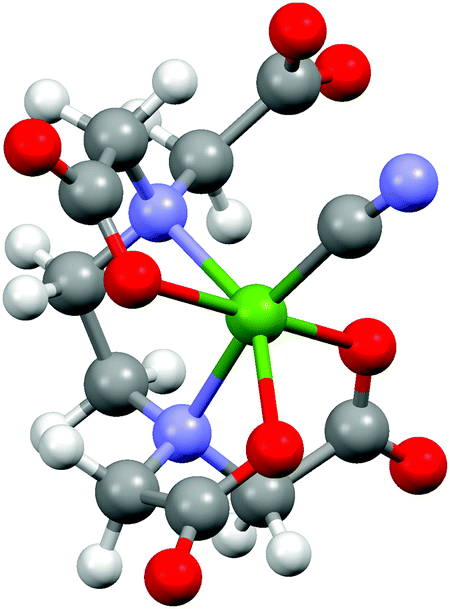Fig. 7 DFT calculated structure of the [NiEDTA(CN)]³⁻ molecular ion (Ni: green, N: blue, O: red, C: grey, H: white).

4 Outlook

A series of Ni–EDTA–CN mixed solutions were studied with laboratory XAS as a function of cyanide concentration in order to reveal the hitherto unresolved structure of hard to observe complexes. While the existence of the pentacyanido coordinated nickel compound was proved unambiguously by the XANES data, an exact structural description is given now for the otherwise inseparable [NiEDTA(CN)]³⁻ mixed ligand complex via fitting the laboratory EXAFS data with a DFT calculation based model.

The present work demonstrates the power of the recently developed laboratory XAS spectrometer prototypes as being capable of measuring synchrotron grade high quality hard X-ray XANES as well as EXAFS spectra of both solid and liquid samples. Laboratory XAS methods show incredible potential for extending the toolbox of researchers in the fields of physical chemistry and chemical physics or even industrial quality control by utilizing the power of high energy resolution X-ray absorption spectroscopies, while bypassing the necessity of applying for synchrotron beamtime and traveling to the synchrotron. They are also excellent when dealing with samples with safety concerns, as safety measures are easier to ensure inside an institute, where a smaller number of staff members need to be involved and made familiar with the possible dangers and necessary preventive procedures. Such instruments could be installed at any laboratory and used to study the electronic-, spin- and structural properties of transition metal based compounds with element selectivity in a condensed state.

Conflicts of interest

There are no conflicts to declare.

Acknowledgements

This work is financed by the ‘Lendület’ (Momentum) Program of the Hungarian Academy of Sciences (LP2013-59), the Government of Hungary and the European Regional Development Fund under Grant VEKOP-2.3.2-16-2017-00015, and the National Research, Development and Innovation Fund (NKFIH FK 124460). ZN acknowledges support from the Bolyai Fellowship of the Hungarian Academy of Sciences. The authors thank László Temleitner for providing the NiSO₄ sample.

References

1. D. Koningsberger and R. Prins, X-Ray Absorption: Principles, Applications, Techniques of EXAFS, SEXAFS and XANES, Wiley & Sons Ltd, 1987.
2. G. T. Seidler, D. R. Mortensen, A. J. Remesnik, J. I. Pacold, N. A. Ball, N. Barry, M. Styczinski and O. R. Hoidn, Rev. Sci. Instrum., 2014, 85, 113906.
3. C. Schlesiger, L. Anklamm, H. Stiel, W. Malzer and B. Kanngießer, J. Anal. At. Spectrom., 2015, 30, 1080–1085.
4. Z. Németh, J. Szlachetko, É. G. Bajnóczi and G. Vankó, Rev. Sci. Instrum., 2016, 87, 103105.
5. D. R. Mortensen, G. T. Seidler, J. J. Kas, N. Govind, C. P. Schwartz, S. Pemmaraju and D. G. Prendergast, Phys. Rev. B, 2017, 96, 125136.
6. I. Mantouvalou, A. Jonas, K. Witte, H. S. R. Jung and B. Kanngießer, X-ray Lasers and Coherent X-ray Sources: Development and Applications, Proc. SPIE, 2017, 10243.
7. W. Malzer, D. Grötzsch, R. Gnewkow, C. Schlesiger, F. Kowalewski, B. Van Kuiken, S. DeBeer and B. Kanngießer, Rev. Sci. Instrum., 2018, 89, 113111.
8. E. P. Jahrman, W. M. Holden, A. S. Ditter, D. R. Mortensen, G. T. Seidler, T. T. Fister, S. A. Kozimor, L. F. J. Piper, J. Rana, N. C. Hyatt and M. C. Stennett, Rev. Sci. Instrum., 2019, 90, 024106.
9. É. G. Bajnóczi, Z. Németh and G. Vankó, Inorg. Chem., 2017, 56, 14220–14226.
10. E. A. Stern and S. M. Heald, Handbook of Synchrotron Radiation: Basic Principles and Applications of EXAFS, North-Holland, 1983, ch. 10, pp. 995–1014.
11. B. Ravel and M. Newville, J. Synchrotron Radiat., 2005, 12, 537–541.
12. J. J. Rehr, J. J. Kas, M. P. Prange, A. P. Sorini, Y. Takimoto and F. Vila, C. R. Phys., 2009, 10, 548–559.
13. S. Graẑulis, A. Daŝkeviĉ, A. Merkys, D. Chateigner, L. Lutterotti, M. Quirós, N. R. Serebryanaya, P. Moeck, R. T. Downs and A. Le Bail, Nucleic Acids Res., 2012, 40, D420–D427.
14. F. Neese, Wiley Interdiscip. Rev.: Comput. Mol. Sci., 2012, 2, 73–78.
15. A. D. Becke, Phys. Rev. A: At., Mol., Opt. Phys., 1988, 38, 3098–3100.
16. J. P. Perdew, Phys. Rev. B: Condens. Matter Mater. Phys., 1986, 33, 8822–8824.
17. A. D. Becke, J. Chem. Phys., 1993, 98, 5648–5652.
18. C. Lee, W. Yang and R. G. Parr, Phys. Rev. B: Condens. Matter Mater. Phys., 1988, 37, 785–789.
19. P. J. Stephens, F. J. Devlin, C. F. Chabalowski and M. J. Frisch, J. Phys. Chem., 1994, 98, 11623–11627.
20. A. Schäfer, H. Horn and R. Ahlrichs, J. Chem. Phys., 1992, 97, 2571–2577.
21. A. Schäfer, C. Huber and R. Ahlrichs, J. Chem. Phys., 1994, 100, 5829–5835.
22. A. Klamt and G. Schüürmann, J. Chem. Soc., Perkin Trans. 2, 1993, 799–805.
23. V. Singh, A. Chetal and P. Sarode, Acta Phys. Pol., A, 1995, 87, 1003.
24. R. L. Mccullough, L. H. Jones and R. A. Penneman, J. Inorg. Nucl. Chem., 1960, 13, 286–297.
25. M. T. Beck, Pure Appl. Chem., 1987, 59, 1703–1720.
26. L. C. Coombs, D. W. Margerum and P. C. Nigam, Inorg. Chem., 1970, 9, 2081–2087.
27. T. Strathmann and S. Myneni, Geochmica et Cosmochimica Acta, 2004, 68, 3441–3458.
28. A. Muñoz-Páez, S. Díaz-Moreno, E. Sánchez Marcos and J. J. Rehr, Inorg. Chem., 2000, 39, 3784–3790.
29. T. F. Sisoeva, V. M. Agre, V. K. Trunov, N. M. Dyatlova and A. Y. Fridman, Zh. Strukt. Khim., 1986, 27, 108.
30. Y. Nesterova and M. Porai-Koshits, Koord. Khim., 1984, 10, 129.
31. D. W. Margerum, T. J. Bydalek and J. J. Bishop, J. Am. Chem. Soc., 1961, 83, 1791–1795.
32. R. D. Shannon, Acta Crystallogr., Sect. A: Cryst. Phys., Diffr., Theor. Gen. Crystallogr., 1976, 32, 751–767.

---

Footnote

† Present address: Department of Molecular Sciences, Swedish University of Agricultural Sciences, Uppsala, Sweden.

---