
 Open Access Article
 This Open Access Article is licensed under a Creative Commons Attribution-Non Commercial 3.0 Unported Licence
Methods for estimating supersaturation in antisolvent crystallization systems†
Jennifer M.
Schall
 ,
Gerard
Capellades
and
Allan S.
Myerson
*
,
Gerard
Capellades
and
Allan S.
Myerson
*
Department of Chemical Engineering, Massachusetts Institute of Technology, 77 Massachusetts Avenue, Cambridge, Massachusetts 02139, USA. E-mail: myerson@mit.edu
First published on 27th August 2019
Abstract
The mole fraction and activity coefficient-dependent (MFAD) supersaturation expression is the least-assumptive, practical choice for calculating supersaturation in solvent mixtures. This paper reviews the basic thermodynamic derivation of the supersaturation expression, revisits common simplifying assumptions, and discusses the shortcomings of those assumptions for the design of industrial crystallization processes. A step-by-step methodology for estimating the activity-dependent supersaturation is provided with focus on ternary systems. This method requires only solubility data and thermal property data from a single differential scanning calorimetry (DSC) experiment. Two case studies are presented, where common simplifications to the MFAD supersaturation expression are evaluated: (1) for various levels of supersaturation of L-asparagine monohydrate in water–isopropanol mixtures and (2) for the dynamic and steady-state mixed-suspension, mixed-product removal (MSMPR) crystallization of a proprietary API in water–ethanol–tetrahydrofuran solvent mixtures. When compared to the MFAD supersaturation estimation, it becomes clear that errors in excess of 190% may be introduced in the estimation of the crystallization driving force by making unnecessary simplifications to the supersaturation expression. These errors can result in additional parameter regression errors – sometimes by nearly an order of magnitude – for nucleation and growth kinetic parameters, limiting the accurate simulation of dynamic and steady-state crystallization systems.
1. Introduction
Crystallization is a rate-based process, so establishing accurate estimates of crystal growth and nucleation rates governs successful crystallization process design and optimization.1–3 Empirically, crystal growth and nucleation are related to supersaturation through power law dependencies, with nucleation generally exhibiting a higher power supersaturation dependence than growth.4 Incorrect estimates of supersaturation lead to incorrect estimates of crystallization kinetics, which result in erroneous predictions of yield, crystal size distribution, and optimal crystallizer operating conditions.By thermodynamic definition, the driving force for crystallization or dissolution arises from a difference between the partial molar Gibbs' free energy of a solute and the chemical potential of the solute at equilibrium. At supersaturated conditions, the solute has a chemical potential of
μ(T) = μ0(T) + RT![[thin space (1/6-em)]](https://www.rsc.org/images/entities/char_2009.gif) ln(a) ln(a) | (1) |
| μsat(T) = μ0(T) + RT ln(asat) | (2) |
Crystallization can occur when the chemical potential of a species is higher than the chemical potential that species would exert at equilibrium. The dimensionless thermodynamic expression for supersaturation is calculated from the difference in chemical potentials as4
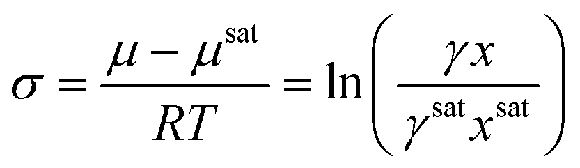 | (3) |
For the rest of this manuscript, this expression will be referred to as the mole fraction and activity coefficient-dependent (MFAD) supersaturation expression. In this expression, four quantities are needed to calculate supersaturation in the solution:
1. xsat, the mole fraction of the solute in the saturated solution. This can be calculated from solubility data.
2. x, the mole fraction of the solute in the supersaturated solution. This can be calculated from mother liquor concentration data.
3. γsat, the activity coefficient of the solute in the saturated solution. This can be calculated from the generalized solubility equation.4
4. γ, the activity coefficient of the solute in the supersaturated solution.
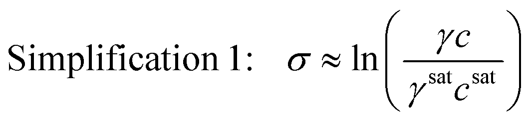
Unfortunately, it is extremely challenging to measure the solute activity coefficient at supersaturated conditions because the system is not at an equilibrium state.5 For this reason, the thermodynamic expression for supersaturation is not immediately useful in industrial settings. This has traditionally led to the use of simplifying assumptions to approximate the true supersaturation of a solution. For example, in dilute systems, the ratio of the solute mole fraction in the supersaturated and saturated phases is close to the ratio of the solute molar concentrations in the supersaturated and saturated phases. This allows to simplify the supersaturation expression as
 | (4) |
This simplification of using concentrations instead of mole fractions is common practice, as it eliminates the need to convert high performance liquid chromatography (HPLC) or other mass-based concentration measurements to solute mole fractions. If the system is also ideal, the activity coefficients are unity, and the supersaturation expression can be simplified even further as
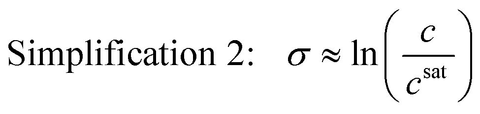 | (5) |
This simplified expression is also acceptable near equilibrium when the ratio of the activity coefficient at supersaturated and saturated conditions is close to unity. For special cases where the supersaturation is also very low (σ ≪ 1) such that ln(σ + 1) = σ, the dimensionless chemical potential difference can be approximated by a dimensionless concentration difference
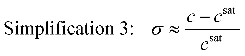 | (6) |
This is generally a poor approximation at σ > 1,6 but it is still normally used despite including the same variables as eqn (5). This simplification brings unnecessary assumptions and should never be used instead of eqn (5).
Simplifications 1–3 imply the assumption that the ratio of solute molar or mass concentrations is equivalent to the ratio of molar fractions between saturated and supersaturated conditions. This assumption only avoids a unit conversion, and it is often flawed when the density and molecular weight of the solute differ from that of the solvent, or when the solute concentrations are high. In those cases, the saturated solution containing lower solute concentrations will have a significantly different density and average molecular weight than the supersaturated system, and the ratio of concentrations will not be equivalent to the ratio of molar fractions.
Simplifications 2 and 3 may also be flawed in highly supersaturated systems. As the system further deviates from ideality, the activity coefficient ratio deviates further from one. This scenario is frequently encountered during batch crystallization and many transient continuous systems. Thus, accounting for the solute activities is often critical for a good prediction of these processes, as well as for the calibration of mathematical models that account for significant variations in supersaturation between experiments. This limitation is more restrictive for antisolvent crystallization, where the activity coefficient ratio quickly deviates from unity even at low supersaturations.
To circumvent the difficulties in measuring the activity coefficient at supersaturated conditions, an estimation method was recently proposed by Valavi, Svärd, and Rasmuson.7 In that method, the activity coefficient in the supersaturated binary solution is assumed to be the same as the activity coefficient in a saturated binary solution of the same composition, allowing the activity coefficient to be approximated using only solubility data and the generalized solubility equation. For these cases, the underlying assumption is that the activity coefficient is a strong function of composition but a weak function of temperature.
In this manuscript, we first present a step-by-step procedure, which builds on the method proposed by Valavi et al.,7 to estimate the MFAD supersaturation in ternary systems. The presented method can also be used for binary systems, although it is especially important for calculating supersaturation during antisolvent crystallization, where both kinetics and thermodynamics are strongly affected by solvent composition.8 With this method, activity-dependent supersaturation estimates may be obtained by pairing solubility data with thermodynamic data from a single differential scanning calorimetry (DSC) experiment. In the second half of the manuscript, we present two case studies to quantify the differences amongst simplifications 1–3, and demonstrate the need for using proper supersaturation estimates.
2. Methods
2.1 Method for estimating MFAD supersaturation in a solvent mixture
The MFAD supersaturation of a solute in a solvent mixture may be estimated using a four-step process. This method works as a reasonable approximation for systems containing a non-charged nonelectrolyte solute. The method is presented for systems presenting a single crystal form. For systems presenting polymorphism, the same steps would have to be repeated for each form to calculate its effective supersaturation. Each polymorph will present different solubilities, melting points and enthalpies of fusion, giving different supersaturation estimates.Theory
For a solute that presents a low vapor pressure in the solid and subcooled liquid states, the generalized solubility equation can be obtained from the fugacity ratio between the solid solute and that of the solute at the subcooled liquid state.4 Assuming that pressure has a negligible effect on solubility, the solubility equation takes the form of: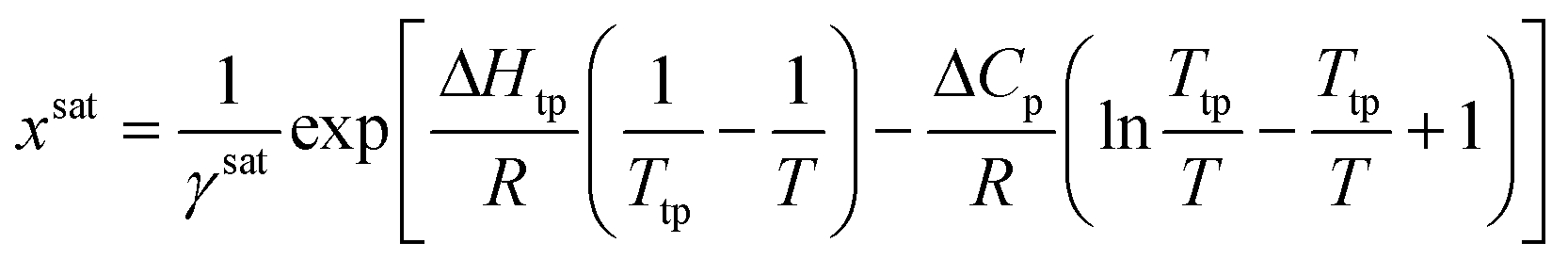 | (7) |
Calculating the system solubility at a given temperature requires knowledge of the activity coefficient at saturation, γsat, the difference in heat capacity between the solid and the subcooled liquid, ΔCp, the enthalpy of change at the triple point, ΔHtp, and the triple point temperature, Ttp. For most systems, ΔHtp and Ttp can be approximated as the enthalpy of fusion and the melting point, respectively.4 Note that these parameters are dependent on the crystal structure, so they are polymorph dependent.
Due to the difficulty of experimentally measuring heat capacities of supercooled liquids, different approximations exist for the estimation of the heat capacity term ΔCp.9 The most common approach is the van't Hoff approximation, where this term is neglected altogether (ΔCp = 0):
 | (8) |
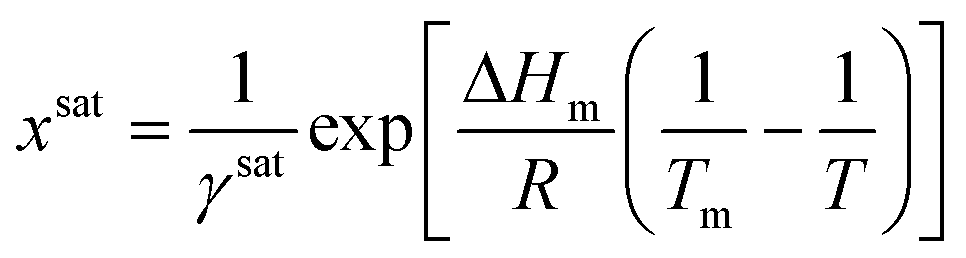
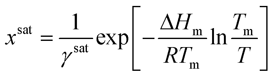
For many systems, a better solution is to approximate the heat capacity term as the entropy of fusion (ΔCp = ΔSm), and assume that this parameter is independent of temperature. At the melting point:
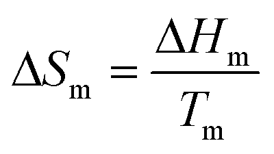 | (9) |
And the general solubility equation reduces to:
 | (10) |
Currently, there is no consensus on which approximation gives the highest accuracy in predicting solubilities, as the results are heavily system-dependent. Mathematically, the van't Hoff approximation works well for systems with low ΔCp, and for systems near their melting point. However, with common organic pharmaceuticals exhibiting differential heat capacities near 100 J mol−1 K−1 and melting points above 400 K,10,11 the van't Hoff approximation would frequently lead to underestimation errors of over 50% for ideal, room temperature solubility.11 Approximating the heat capacity term as the entropy of fusion gives a more accurate approach than neglecting this term altogether. Alternative approaches are based on measuring the temperature-dependent heat capacities of the solute in the solid phase and in the melt, and using extrapolation of the melt heat capacity to estimate ΔCp.10
The methods provided in this work approximate ΔCp as the entropy of fusion, using eqn (10) as a simple expression for estimating activity coefficients along the solubility curve. This method was chosen because it is a simple alternative for the calculation of activity coefficients using limited amounts of data. Note that the estimated MFAD supersaturations depend on a ratio of activities rather than their absolute value. Consequently, estimations of supersaturation are significantly less sensitive to errors in the heat capacity term than estimations of ideal solubilities. A detailed error propagation study is provided in ESI,† where the impact of estimation errors in the heat capacity term are evaluated for four common pharmaceuticals with significantly different thermal properties.
Summary of assumptions:
1. Pressure has a negligible effect on solubility.2. At the temperature range of interest, the solute presents a negligible vapor pressure in both the solid and subcooled liquid states.
3. The solute's triple point temperature and the enthalpy of change for the liquid solute transformation at the triple point can be approximated as the melting point and the enthalpy of fusion, respectively.
4. The differential heat capacity between the solid solute and its melt, ΔCp, has a negligible temperature dependence, and it can be approximated as the solute's entropy of fusion.
5. The incorporation of solvents and impurities in the crystalline phase is negligible.
6. The activity coefficients exhibit a small dependence on temperature over a moderate temperature range.12
Step 1. Data collection
1. Complete a DSC experiment on a crystallized solute sample to determine the enthalpy of fusion, ΔHm, and the melting point, Tm. Alternatively, these values may be obtained from literature if available.2. Determine the solute solubility as a function of temperature and solvent composition throughout the operating range of interest. Convert the solubility data to a molar basis.
3. Establish a relationship between API solubility, solvent composition, and temperature. Any combination of appropriate solubility models may be used when regressing solubility parameters, as long as they accurately capture the effects of temperature on solubility. The examples provided in this work are based on a modified Apelblat equation that takes into account the effects of both temperature and solvent composition on solubility.8 For binary systems or antisolvent crystallization at fixed solvent fractions, only a solubility curve as a function of temperature would be needed.
At this point, the regressed solubility model can estimate xsat as a function of temperature and solvent composition throughout the operating range. Steps 2–4 describe how to calculate the MFAD supersaturation for a given data point, provided that the system temperature, solvent composition and solute concentration are known.
Step 2. Calculating activity coefficient at saturation
1. Calculate the solubility at the operating temperature and solvent composition, xsat, using the selected solubility model.2. Use the general form of the solubility equation to calculate the activity coefficient at saturation:
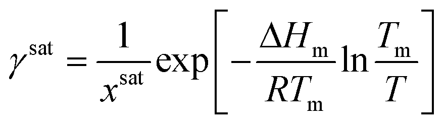 | (11) |
Step 3. Estimating activity coefficient at supersaturated conditions
1. Solve the regressed solubility expression for temperature using the solute concentration and the solvent fraction in the crystallizer.7 This calculated temperature, Te, will be referred to as the ‘effective’ solubility temperature, and it is the saturation temperature for the operating solute concentration.2. Using the effective temperature, Te, and the solute concentration in the crystallizer, x, solve the general form of the solubility equation to estimate the activity coefficient at supersaturated conditions:
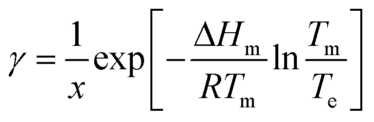 | (12) |
This approximation is based on the assumption that the activity coefficients are a weak function of temperature and a strong function of solute concentration, as previously demonstrated by Valavi et al.7 Following this assumption, the activity coefficients at supersaturated conditions can be approximated as those in a saturated system at the same composition.
Step 4. Calculating supersaturation
1. Calculate the MFAD supersaturation according to the thermodynamic definition for supersaturation: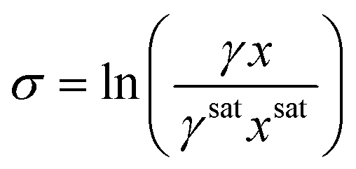 | (13) |
At this point, we can now estimate thermodynamic supersaturations at any point during the course of an experiment from given crystallizer operating conditions, mother liquor concentration, and solute physical property data.
2.2 System descriptions for case study compounds
To test the application of the proposed MFAD supersaturation estimation method, we considered two systems as case studies.For both systems, a 12-parameter modified Apelblat model was used to estimate solubility because neither system exhibits solubility extrema in the operating range, and we previously determined the solubility parameters for one of the case study compounds systems using this equation.13,14 By using this expression, it is assumed that the enthalpy of the solution is proportional to the solution temperature.15 The equation for the modified Apelblat solubility model is:
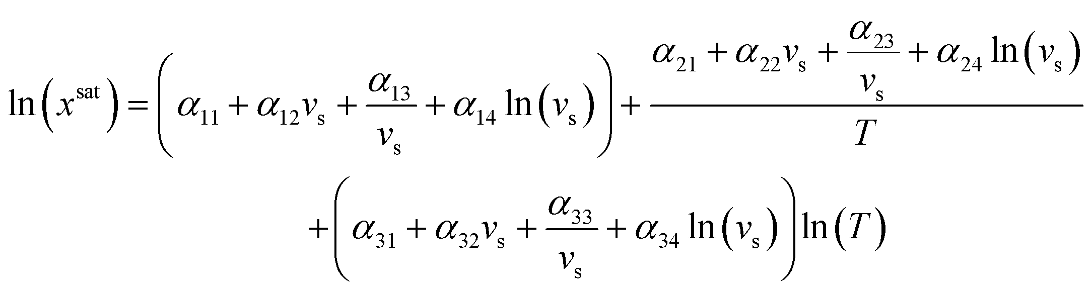 | (14) |
For the first case study, we studied L-asparagine monohydrate (LAM) in isopropanol (IPA)/water mixtures, where water is the solvent and IPA is the antisolvent. LAM solubility as a function of temperature and solvent composition was obtained from literature, along with thermal property data for melting temperature and enthalpy of fusion.16 This compound's enthalpy of fusion is on the higher end compared to common organic crystallization solutes,10 presumably because LAM is decomposing near the melting point.17 However, because it is difficult to decouple melting from decomposition in calorimetry studies, this is the most accurate measurement that is currently available. The regressed solubility parameters for the LAM system are provided in Table 1.
| j↓/k→ | 1 | 2 | 3 | 4 |
|---|---|---|---|---|
| 1 | 3539.6 | −4110.5 | 660.4 | 3645.7 |
| 2 | −174415.1 |
197949.6 |
−31558.5 |
−174717.4 |
| 3 | −520.4 | 605.9 | −97.5 | −537.5 |
The purpose of using this system was to evaluate how the proposed supersaturation estimation method compares with common supersaturation approximations over a wide range of supersaturations and solvent fractions. For these calculations, supersaturation estimations were made at a series of temperature, solvent composition, and hypothetical operating concentrations for LAM. The parameter space for these selected conditions is provided in Table 2. In some cases, the simulated solutions required an estimation of effective temperature which lies outside of the range of temperatures encompassed by the solubility model. At these conditions, the supersaturation estimations were disregarded.
| Variable | Min value | Max value | Units |
|---|---|---|---|
| Temperature | 25 | 55 | °C |
| Solvent (water) volume fraction | 20 | 100 | v% |
| Supersaturated LAM mole fraction | 0.0001 | 0.015 | mol/mol |
For the second case study, we considered a proprietary compound produced by Novartis. This compound is crystallized in ethanol (EtOH)/tetrahydrofuran (THF)/water mixtures, where a solution of 92 v% EtOH/8 v% THF serves as the solvent and water serves as the antisolvent. Throughout this paper, the proprietary compound will be referred to as API. Thermal property data were provided by Novartis International AG, and the solubility measurements were described elsewhere.8 The parameter values for this solubility model are reproduced in Table 3. Instead of estimating supersaturation and solubility at a variety of potential operating conditions, data from previous dynamic and steady-state, continuous MSMPR experiments were used.8
| j↓/k→ | 1 | 2 | 3 | 4 |
|---|---|---|---|---|
| 1 | −7889.3 | 12288.8 |
−4942.5 | −16439.8 |
| 2 | 331574.5 |
−520921.6 |
211152.4 |
700687.6 |
| 3 | 1190.5 | −1854.0 | 744.8 | 2479.1 |
For both model systems, the bulk of the calculations described in section 2.1 was conducted using gPROMS Formulated Products. Details on the process variables and parameter values for both systems can be found in ESI.†
To quantitatively assess the errors of simplifications 1–3, the percent difference between the MFAD expression and each simplifying supersaturation expression was calculated using the following formula:
 | (15) |
3. Results and discussion
3.1 Case study 1: LAM in water–IPA mixtures
Fig. 1 provides a comparison of each simplified supersaturation expression with the proposed supersaturation evaluation method. Immediately, it is apparent that simplifications 2 and 3 do not provide acceptable estimates of supersaturation, as they experience strong deviations from the thermodynamic estimation of the supersaturation driving force. These deviations, quantified from eqn (15), show that simplification 2 has errors of between 19.3% and 62.1% when compared with the method presented in this paper, and this deviation increases with supersaturation. These deviations are attributable to the non-ideality of the antisolvent system and will always be negative because the activity coefficient ratio is greater than one for a supersaturated solution. Simplification 3 has a similar range of error, ranging from 0.08% to 59.3%. Simplification 1, however, appears to provide an acceptable estimate of supersaturation for this system, with errors ranging from 0.03% to 3.4%. The close agreement between the MFAD supersaturation expression and simplification 1 exists because the concentration of LAM in the system is not substantially high (with an LAM mole fraction of less than 0.013 in all cases). However, note that the small error between the MFAD supersaturation expression and simplification 1 is not generalizable to every system. Considering that simplification 1 only avoids a unit conversion, we do not recommend using this simplification as general practice.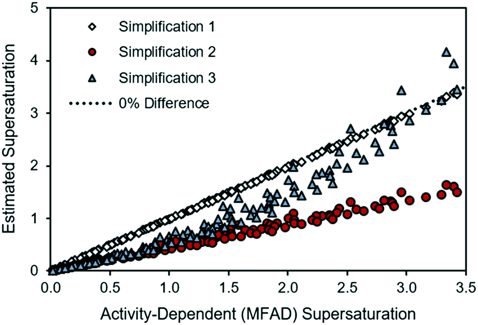 | ||
| Fig. 1 Comparison of simplified supersaturation with MFAD supersaturation calculations for LAM system. | ||
3.2 Case study 2: application to proprietary API in ethanol/THF/water solutions
In this case study, the supersaturation was calculated for each simplified expression using concentration, temperature, and solvent composition data from each of four continuous MSMPR runs completed using a proprietary compound from Novartis International AG.8 Similar estimation errors were observed in each run, as summarized in Table 4.| Run | Simplification 1 | Simplification 2 | Simplification 3 | |||
|---|---|---|---|---|---|---|
| Min | Max | Min | Max | Min | Max | |
| 1 | 0.01% | 0.35% | 26.8% | 36.6% | 1.46% | 82.8% |
| 2 | 0.27% | 1.61% | 25.4% | 35.4% | 0.44% | 69.2% |
| 3 | 0.00% | 1.23% | 18.3% | 50.1% | 15.6% | 192% |
| 4 | 0.04% | 1.04% | 0.93% | 41.4% | 3.80% | 113% |
As an example, the following discussion will be based on run 3, where the MSMPR was operated at a solvent volume fraction of 48 vol% and a residence time of 90 min. For the first portion of run 3, the crystallizer temperature was controlled at 10 °C. A constant temperature and solvent composition was sustained until the system reach steady state. Then, starting at 900 minutes, the crystallizer temperature was changed to 30 °C and a new steady state was reached at the same solvent composition. This run was chosen as it presented the broadest range of supersaturations.
During the start-up phase, both low supersaturations and high supersaturations are experienced as the system undergoes rapid initial supersaturation development and transitions to steady-state operation. Fig. 2 shows that the estimation errors for supersaturation are a function of the system concentration, with supersaturation spikes being heavily overpredicted by simplification 3. This behavior not only limits the ability to predict transient MSMPR kinetics, but also increases the uncertainties during parameter estimation (for both batch and MSMPR crystallization). Simplification 2 followed a similar trend as the MFAD supersaturation, with a consistent underprediction of the crystallization driving force.
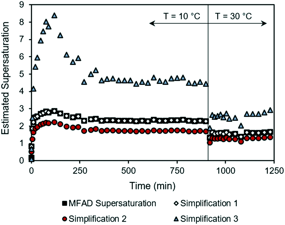 | ||
| Fig. 2 Supersaturation trajectories for dynamic MSMPR run 3, as calculated using the MFAD and simplified supersaturation expressions. | ||
For comparison with the LAM case study in Fig. 1, the experimental API supersaturations have been plotted against the MFAD supersaturation values in Fig. 3.
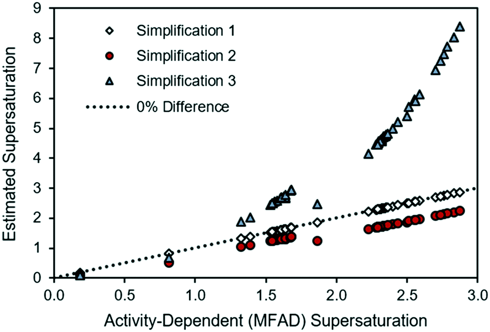 | ||
| Fig. 3 Comparison of supersaturations calculated using the MFAD and simplified supersaturation expressions for MSMPR run 3. | ||
For the case of API, and as it occurred for the LAM system, the agreement between the MFAD expression and simplification 1 appears acceptable because, with typical mother liquor concentrations of approximately 3 mg g−1 solution, API does not comprise a substantial portion of the solution.
Simplification 2 consistently shows a substantial, negative deviation from the MFAD supersaturation. Finally, simplification 3 shows both positive and negative deviations from the MFAD supersaturation, indicating that it is the most inconsistent method of estimating the crystallization driving force.
Especially during process design, where kinetic orders are being regressed for significantly different supersaturations, a wrong estimation of supersaturation will increase the uncertainty of the regressed parameters. Semi-empirical power law kinetic expressions for nucleation and crystal growth typically take the form of:
| G = kgσg | (16) |
| B = kbσbMTj | (17) |
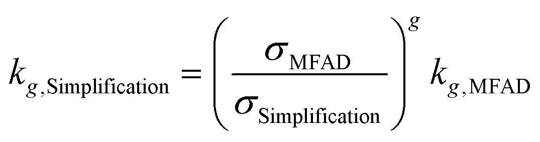 | (18) |
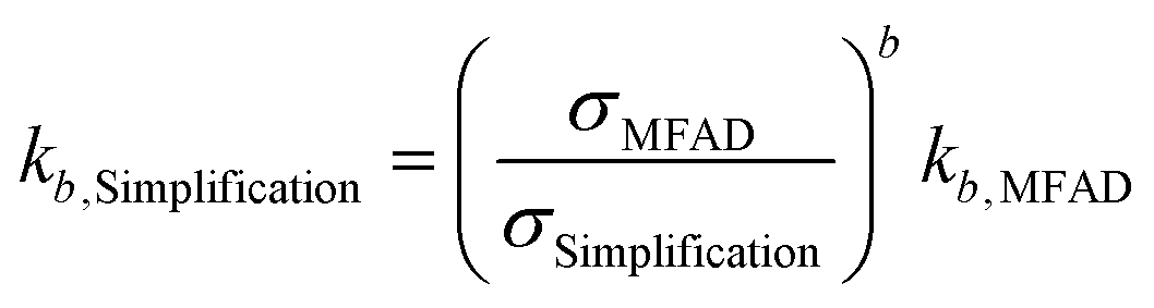 | (19) |
For the data presented for run 3, and assuming values of g = 1 and b = 2, the differences in estimated kinetic parameters for each simplification are summarized in Table 5.
| Simplification | k g,Simp/kg,MFAD | k b,Simp/kb,MFAD | ||
|---|---|---|---|---|
| Min | Max | Min | Max | |
| 1 | 0.99 | 1.00 | 0.98 | 1.00 |
| 2 | 1.22 | 2.00 | 1.50 | 4.01 |
| 3 | 0.34 | 1.91 | 0.12 | 3.66 |
Note that kinetic parameter estimates for nucleation are affected to a greater extent by incorrect estimations of supersaturation due to the higher nucleation kinetic order b. The higher errors are observed for estimating kb using simplification 3. Here, the estimated parameter is only 12% of the real value, leading to a prediction error of nearly an order of magnitude. Carrying through these erroneous predictions of supersaturation and kinetic parameters to crystallizer design, optimization, and performance prediction will result in yield and PSD calculation errors, as well.
4. Conclusions
Supersaturation estimates are highly dependent on the underlying supersaturation expression assumptions. Many of the traditional assumptions regarding supersaturation calculations, such as having a low supersaturation or having an activity coefficient ratio of one at supersaturated conditions, do not apply to antisolvent or mixed-solvent systems. The least restrictive set of assumptions regarding supersaturation calculations involves calculating supersaturation as a function of solute mole fraction and activity coefficient at supersaturated and saturated conditions (eqn (3)).Building on the method originally presented by Valavi et al.,7 supersaturated activity coefficients in mixed-solvent systems were estimated using only solubility and DSC data by computing an effective temperature and using that temperature in the generalized solubility equation to approximate the activity coefficient at supersaturated conditions. The presented method is especially recommended for crystallization from mixed solvent systems or for processes dealing with large variations in supersaturation (e.g. batch and some transient continuous crystallizers). If simplifying assumptions are used, it is strongly recommended to employ the logarithmic supersaturation expression using solute mole fractions for concentration, and not molar concentrations or mass fractions. Other assumptions only increase the complexity of supersaturation determination by a small margin, but they can significantly increase the uncertainties on the determination of the crystallization driving force.
Nomenclature
| a | Activity of solute at supersaturated conditions |
| a sat | Activity coefficient of solute at saturated conditions |
| B | Nucleation rate |
| b | Nucleation rate order for supersaturation |
| c | Concentration of solute at supersaturated conditions, typically expressed on total solution mass or on total solution volume basis |
| c sat | Solute solubility, typically expressed on total solution mass or on total solution volume basis |
| G | Growth rate |
| g | Growth rate order for supersaturation |
| j | Nucleation rate order for suspension density |
| k g | Temperature-dependent growth rate factor |
| k b | Temperature-dependent nucleation rate factor |
| M T | Suspension density |
| R | Ideal gas constant |
| T | Temperature |
| T e | Effective temperature |
| T m | Melting point temperature |
| T tp | Triple point temperature |
| v s | Solvent volume fraction |
| x | Mole fraction of solute at supersaturated conditions |
| x sat | Mole fraction of solute at saturated conditions (mole fraction solubility) |
| α jk | Modified Apelblat solubility parameter |
| Δcp | Differential heat capacity between the solid solute and the hypothetical supercooled melt |
| ΔHm | Solute's enthalpy of fusion |
| ΔHtp | Solute's enthalpy of change at the triple point |
| ΔSm | Solute's entropy of fusion |
| ε | Estimation error |
| γ | Activity coefficient of solute at supersaturated conditions |
| γ sat | Activity coefficient of solute at saturated conditions |
| μ | Chemical potential of the solute |
| μ sat | Chemical potential of the solute at saturated conditions |
| μ 0 | Chemical potential of the solute at a reference state |
| σ | Dimensionless supersaturation |
Conflicts of interest
There are no conflicts to declare.Acknowledgements
We thank the Novartis-MIT Center for Continuous Manufacturing for funding and technical guidance. We also acknowledge the National Science Foundation, Grant No. 1122374, for funding. Any opinion, findings, and conclusions or recommendations expressed in this material are those of the authors and do not necessarily reflect the views of the National Science Foundation.Notes and references
- B. J. Ridder, A. Majumder and Z. K. Nagy, Ind. Eng. Chem. Res., 2014, 53, 4387–4397 CrossRef CAS.
- G. Power, G. Hou, V. K. Kamaraju, G. Morris, Y. Zhao and B. Glennon, Chem. Eng. Sci., 2015, 133, 125–139 CrossRef CAS.
- Y. Yang and Z. K. Nagy, Ind. Eng. Chem. Res., 2015, 54, 5673–5682 CrossRef CAS.
- A. S. Myerson, Handbook of Industrial Crystallization, Butterworth-Heinemann, 2nd edn, 2002 Search PubMed.
- H.-S. Na, S. Arnold and A. S. Myerson, J. Cryst. Growth, 1995, 149, 229–235 CrossRef CAS.
- S. Kim and A. S. Myerson, Ind. Eng. Chem. Res., 1996, 35, 1078–1084 CrossRef CAS.
- M. Valavi, M. Svärd and A. C. Rasmuson, Cryst. Growth Des., 2016, 16, 6951–6960 CrossRef CAS.
- J. M. Schall, J. S. Mandur, R. D. Braatz and A. S. Myerson, Cryst. Growth Des., 2018, 18, 1560–1570 CrossRef CAS.
- S. H. Yalkowsky and M. Wu, J. Pharm. Sci., 2010, 99, 1100–1106 CrossRef CAS PubMed.
- S. H. Neau, S. V. Bhandarkar and E. W. Hellmuth, Pharm. Res., 1997, 14, 601–605 CrossRef CAS PubMed.
- G. D. Pappa, E. C. Voutsas, K. Magoulas and D. P. Tassios, Ind. Eng. Chem. Res., 2005, 44, 3799–3806 CrossRef CAS.
- J. M. Prausnitz, R. N. Lichenthaler and E. G. DeAzevedo, Molecular thermodynamics of fluid-phase equilibria, Prentice-Hall, Englewood Cliffs, NJ, 1986 Search PubMed.
- E. Manzurola and A. Apelblat, J. Chem. Thermodyn., 2002, 34, 1127–1136 CrossRef CAS.
- M. Jabbari, N. Khosravi, M. Feizabadi and D. Ajloo, RSC Adv., 2017, 7, 14776–14789 RSC.
- A. Apelblat and E. Manzurola, J. Chem. Thermodyn., 1997, 29, 1527–1533 CrossRef CAS.
- M. Lenka and D. Sarkar, Fluid Phase Equilib., 2016, 412, 168–176 CrossRef CAS.
- M. Contineanu, A. Neacsu, I. Contineanu and S. Perisanu, J. Radioanal. Nucl. Chem., 2013, 295, 379–384 CrossRef CAS.
Footnote |
| † Electronic supplementary information (ESI) available: Summary of gPROMS model equations, parameters and variables. Error propagation study. See DOI: 10.1039/c9ce00843h |
| This journal is © The Royal Society of Chemistry 2019 |