Optimization and quantification of the systematic effects of a rolling circle filter for spectral pre-processing

Abstract

Spectral pre-processing, especially baseline approximation, is a crucial part in quantitative spectroscopic applications, such as Raman or FTIR spectroscopy. Filters used for this task need to be optimized for their application, in order to achieve a sufficient baseline approximation while minimizing the distortion of the spectral lines. We propose a combined method that optimizes a rolling circle filter and quantifies the residual systematic influence on the spectral lines by a Monte Carlo approach that simulates and subsequently analyses spectra with known line properties and known maximum baseline curvature.

---

1 Introduction

A typical spectrum consists of a signal that contains features relevant for the spectroscopic application and the non-relevant background and noise. The background can be further classified into two groups: first, the smooth low-frequency baseline caused for example by instrumental effects, such as the source intensity or beam splitter transmission in FTIR, or the fluorescence background in Raman; second, sharp high-frequency background signals or bands caused for example by atmospheric absorption. The goal of spectral pre-processing is to separate the relevant signal from the background. By the separation of the signal and background, baseline removal techniques allow quantitative studies based on spectroscopy. Common applications are, e.g. the investigation of molecular energy levels¹ or concentration measurements based on line intensities or absorbances.^2–4

An excellent overview of baseline-removal techniques is given by H. G. Schulze et al.,⁵ containing e.g. polynomial or spline approximation methods, band-pass filters or derivative methods. Fully automated pre-processing methods have been implemented using the Savitzky–Golay⁶ or second derivative methods.⁷ The Savitzky–Golay filter⁸ is a smoothing-filter that obtains results similar to a moving average. Therefore, the filter tends to deliver uneven baselines. Modifications to improve this behaviour, e.g. as proposed by H. G. Schulze et al.,⁶ are time consuming just like the smoothing splines used by the second derivative method presented by C. Rowlands and S. Elliott.⁷

In this work, we use a geometrical rolling circle filter for baseline estimation. This filter was originally published by I. K. Mikhailyuk and A. P. Razzhivin.⁹ They demonstrated its application to 1-dimensional data in the form of Raman spectra and chromatograms and 2-dimensional electrophoresis patterns. The rolling circle filter for baseline-removal is commonly used in spectroscopic techniques based on Raman spectroscopy, such as composition analysis via micro-Raman spectroscopy of algae^10,11 or the investigation of the structural phase transition of vanadium dioxide.¹² For the continuous in-line concentration monitoring of hydrogen isotopologue mixtures, James et al.¹³ implemented a fully automatic spectral analysis based on a slightly modified rolling circle filter in combination with a Savitzky–Golay filter. Our application is the development of a real-time and inline measurement system for the concentration of liquid hydrogen isotopologues for the integration in a cryogenic distillation column in the fusion fuel cycle.^3,4,14 We use the original rolling circle filter and apply it on the FTIR spectra of liquid hydrogen isotopologues, which delivers a sufficient baseline-removal without the necessity of an additional Savitzky–Golay filter for the characteristic background curvatures and peak shapes of these spectra.

In FTIR spectroscopy, a division by a reference spectrum, recorded with only the solvent in the measuring cell is typically used for baseline removal. However, in the case of gases or pure liquids as the sample, a smooth baseline remains to be removed after this division, which implies the use of a filter for pre-processing before the actual analysis. The parameters of the filter need to be optimized, depending on its application, to minimize the distortion of the spectral lines and preserve the important parameters for spectra analysis, namely the peak position, peak intensity (height or integral) and peak width. Since this optimization cannot completely avoid the distortion effects, the systematic influence of the filter on the peak parameters needs to be known, to be used either as a systematic uncertainty or for correction. We present a method, demonstrated on the example of a rolling circle filter, that both optimizes the filter and quantifies its systematic influence on the peak parameters namely width, intensity and position.

2 Two-dimensional parameter optimization of the rolling circle filter by a least squares method

The rolling circle filter,⁹ which is the subject of this study, can be described in three steps. First, a circle with radius r is constructed for each point of the input spectrum, with the x-coordinate of this point being the x-coordinate of the center of the circle. This corresponds to the circle rolling over the spectrum. Second, the circle touches the spectrum in at least one point, but never intersects it. The circle touches from below, if the signals are positive, and from above, if the signals are negative. In the following, only the procedure for negative signals is discussed. Third, the difference of the input spectrum and the circle's lower arc is calculated. This value is compared with the corresponding y-coordinates in the output array. The higher value is written to the output array. This comparison is repeated for each point of the input spectrum and its corresponding circle. The output array then represents the constructed baseline.

Since the circle radius strongly defines this baseline and needs to be adapted to the curvature of the input spectrum, it is indispensable to optimize this parameter depending on the application of the filter.

2.1 Optimization method

This optimization method for filter parameters uses the sum of squared differences of the extracted baseline t([small nu, Greek, tilde])_b and the unfiltered transmission spectrum t([small nu, Greek, tilde]) as the characteristic parameter. This method was already proposed by I. K. Mikhailyuk and A. P. Razzhivin⁹ and implemented by N.N. Brandt et al.¹⁵ In the case of the rolling circle filter, according to Mikhailyuk and Razzhivin,⁹χ² shows a plateau at certain radii, with the ideal filter radius being on the plateau, close to the right edge.

This plateau is created by the following effects:

• for small radii r_{[small nu, Greek, tilde]}, the filter-circle rolls into the signal peaks, therefore χ² is small.

• for intermediate radii r_{[small nu, Greek, tilde]} – the plateau – the filter eliminates the background. Its radius is larger than the peak width, but smaller than the background curvature, therefore χ² increases only slowly with increasing filter radius.

• For large radii r_{[small nu, Greek, tilde]}, the baseline detaches from the spectrum, as the filter radius becomes larger than the spectrum's curvature, leading to a rapid increase in χ².

We also use the rolling circle filter for the presented optimization, however we apply three modifications in comparison to Mikhailyuk and Razzhivin.

First, we use the rolling circle filter for transmission spectra in absorption spectroscopy and therefore negative signals.

Second, we normalize the spectra to their value at the wavenumber 2500 cm⁻¹.

Third, we use an ellipse instead of a circle, and therefore characterize our filter by two parameters. This allows us to minimize the calculation time, as the calculation-time depends on the size of the arrays holding the spectrum and the circle shape.

Since this extends our optimization problem to two dimensions r_{[small nu, Greek, tilde]} and r_T, χ² is represented by a matrix (dimension n × m). We can improve the search for kinks and the plateau in this matrix by analyzing the norm of the corresponding Hessian matrices for each element of the χ² matrix. The Hessian matrices (dimension m × n = 2) are calculated from each element of the chi squared matrix according to . We then calculate the sub-multiplicative max-norm for each Hessian matrix. This results in a (n − 2) × (m − 2) matrix sensitive to the edges of the plateau in the χ² matrix.

2.2 Result: determination of optimized filter parameters

To illustrate the previously discussed optimization method, we chose the second vibrational branch of an absorption spectrum of a liquid hydrogen–deuterium mixture. We performed the described algorithm on this for 50 values in the parameter intervals given in Table 1.

Table 1 Input parameters for the rolling circle filter optimization

Parameter	Min.	Max.
r [small nu, Greek, tilde] (cm^−1)	100	9000
r I	0.1	25
[small nu, Greek, tilde] (cm^−1)	5800	12 000

---

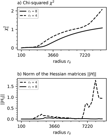
Fig. 1 shows χ² and the corresponding norms of the Hessian matrices for these parameter intervals. The edges of the plateau, which quadratically depend on the [small nu, Greek, tilde] and T-radius, are clearly visible in the norm of the Hessian matrix. To illustrate the determination of the ideal rolling circle filter radius, Fig. 2 shows the χ² dependency on the radius r_{[small nu, Greek, tilde]} for a fixed radii r_T. Between the [small nu, Greek, tilde]-radii of approximately 500 cm⁻¹ and 1350 cm⁻¹ for r_T = 4.0 and 500 cm⁻¹ and 2000 cm⁻¹ for r_T = 8.0 the previously discussed plateau in the χ² dependency is visible. This shows that a smaller T-radius can be compensated by an also smaller radius in the [small nu, Greek, tilde] direction.

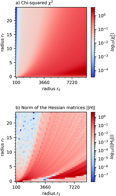Fig. 1 The χ² matrix (a) and the corresponding norms of the Hessian matrices of the χ² matrix ‖H‖ (b).

Fig. 2 The χ² (a) and the corresponding norms of the Hessian matrices of the χ² matrix ‖H‖ (b) at the fixed radii r_T = 4 and r_T = 8. Note the plateau between 500 cm⁻¹ and 1350 cm⁻¹ at 2000 cm⁻¹ and the second edge at r_{[small nu, Greek, tilde]} = 6000 for r_T = 4. The ideal filter radius is the point, where, beginning at small radii, ‖H‖ starts to differ from zero.

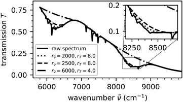
For the radius r_T = 4.0, χ² shows a second plateau with the right edge at approximately r_{[small nu, Greek, tilde]} = 6000. To investigate its origin, we filtered a spectrum used for this optimization with different filter radii, see Fig. 3. The hereby determined baselines show a beginning detachment from the peak edges at the filter radii of r_{[small nu, Greek, tilde]} = 2500 and r_T = 8.0.

Fig. 3 Comparison of baselines created by the rolling circle filter at different parameters r_{[small nu, Greek, tilde]} and r_T for the first vibrational overtone band of a transmission spectrum of a liquid hydrogen deuterium mixture.

The baseline created with the radii of r_{[small nu, Greek, tilde]} = 6000 and r_T = 4.0 corresponds to the right edge of the second plateau in the χ² dependency at a fixed r_T = 4.0. For this larger filter ellipse, the baseline completely detaches from the peaks between [small nu, Greek, tilde] = 5800 cm⁻¹ and [small nu, Greek, tilde] = 6800 cm⁻¹ and [small nu, Greek, tilde] = 7800 cm⁻¹ and [small nu, Greek, tilde] = 9100 cm⁻¹. At these radii, the rolling circle filter is unable to create a baseline that compensates for the curvature that is caused by the transmission function of the KBr beam-splitter used in the FTIR spectrometer for the recording of this spectrum.

In conclusion, the right edge of the left plateau with the radii r_{[small nu, Greek, tilde]} = 2000 and r_T = 8.0, or similarly r_{[small nu, Greek, tilde]} = 1350 and r_T = 4.0, serves as an ideal radius according to our optimization procedure.

2.3 Discussion

The results of the optimization of the rolling circle filter performed exemplarily show the importance of this procedure concerning three points.

First, the optimal filter parameters enable the determination of a baseline for the filtered spectrum that minimizes the distortion of the spectral lines.

Second, as seen in Fig. 3, the optimal filter parameters prevent a detachment of the baseline from the spectrum in regions with high curvature. Depending on the spectrum, the optimal filter parameters are not necessarily represented by the global maximum, but rather by local maxima, in the matrix of the norms of the Hessian matrices of the χ² matrix, and therefore, a careful selection of filter parameters is necessary.

Third, regarding the rolling circle filter, the optimal parameter curve in the T-[small nu, Greek, tilde] radius space enables us to choose a small [small nu, Greek, tilde] radius and therefore allows us to minimize the calculation time.

In a real spectrum, not only the line width and intensity, but also the baseline's curvature varies. Therefore, a simple optimization of a filter for spectral pre-processing cannot be performed on a single line, but has to be obtained for the spectral part that is the subject of the investigation. However, the result of such an optimization leads to a parameter set that is only optimal for an average line. Therefore, some lines are filtered perfectly, for some lines, the baseline doesn't touch the peak edges in the case of neighboring lines and for some lines, the baseline is already subtracting the actual peak area. The first effect is minimized by the division of the sample spectrum by a reference spectrum, in case the baseline's curvature is caused by an instrumental effect. The second effect, however, cannot be prevented if a single filter parameter set is used for lines with different widths. Therefore, the quantification of this effect is indispensable, if the line absorbance and width are the subject of the spectroscopic investigation.

3. Quantification of the influence of a filter on the line-shape in the example of the rolling circle filter

The aim of this study is to quantify the systematic influence of the rolling circle filter on the peak shape, in order to determine and correct the systematic uncertainty introduced by the rolling circle filter. Especially relevant are the parameters that represent the position, width and intensity or absorbance of the peak. These parameters serve as a measurand in spectroscopic investigations.

To study the systematic influence of the filter on these, we implemented a method based on the simulation of random peaks on a random background. We set the constraint that the parameters defining the background and peaks are chosen randomly, but in a defined range. These spectra are then treated with the rolling circle filter and the peaks are analyzed to extract their parameters after filtering. There are three main reasons to rely on statistics, rather than doing a specific analysis for this simulation.

First, the correlations between the peak and background parameters and the influence of the filter on these are unknown beforehand. Therefore, since it is not known which input parameters lead to which result, direct non-randomized analysis is not possible.

Second, this method is intended as a general method not only applicable for one filter. For a specific filter, there might be specific methods to investigate possible correlations, a universal method however needs to rely on statistics.

Third, usually in a spectroscopic application, the final filtered spectrum is the result that is used to determine the peak width, integral and position. Therefore, the systematic influence on the peak shape must be known on the basis of the already filtered peak. A method based on statistics provides suitable tools to achieve this.

3.1. Determination of input parameters for the simulation from measured spectra

The simulation needs two different sets of input data: background related and peak related parameters. The relevant parameters characterizing the background shape b([small nu, Greek, tilde]) are its gradient m([small nu, Greek, tilde]) = b’([small nu, Greek, tilde]) and curvature .¹⁶ We determined the maximum curvature as the input parameter from the measured spectra by extracting a baseline with the rolling circle filter and a numerical calculation of the curvature for every point of the baseline. We determined then the line parameters width σ, position μ and intensity I by the typical selection of spectral lines from the second vibrational branch of the liquid hydrogen isotopologues, see Table 2, and then a manual determination of the respective parameters. The hereby determined input parameter ranges, including a certain margin, are given in Table 3.

Table 2 Selected lines and the corresponding parameters intensity I, width σ and center μ determined from the experimentally measured FTIR spectra of the inactive hydrogen isotopologues

Line	μ (cm^−1)	I	σ
L35	6644.8	0.008	6.7
L43	7156.9	0.018	3.0
L52	8858.6	0.038	20.1
L62	8868.3	0.064	7.4

---

Table 3 Input parameter ranges for the spectral simulation determined from the measured spectra

Parameter	Minimum	Maximum
κ	—	2.15 × 10^−6
μ	6050	9750
Σ	2	50
I	0.001	1

---

3.2. Simulation method

As the peak, we chose a simple Gaussian shape , scaled by the factor I, with the Gaussian width σ and the center wavenumber of the peak μ. This shape is symmetric, therefore an asymmetric contribution introduced by the rolling circle filter can be easily quantified. Also, the shape is only defined by three parameters, which leads to a better stability for the fitting of this shape to the filtered spectra. The peak parameters were chosen randomly in the parameter range given in Table 3.

We place the simulated peaks on a random cubic spline background only defined by its maximum curvature. This kind of background b([small nu, Greek, tilde]) is generated by randomly choosing curvature values with a given maximum absolute value. These curvature values are interpolated with cubic splines resulting in the curvature κ([small nu, Greek, tilde]). The non-linear second order differential equation for the background

b′′([small nu, Greek, tilde]) = κ([small nu, Greek, tilde])(1 + b′([small nu, Greek, tilde])²)^3/2 (1)

is then solved numerically using a Runge–Kutta¹⁷ method. Here the initial values are chosen to be ∀n ∈ [Doublestruck N]⁰:b⁽ⁿ⁾(0) = 0.

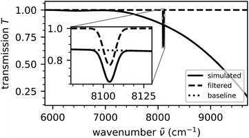
For simplicity and to avoid overlaps, we restrict the simulation to a single peak per spectrum. An example of a transmission spectrum simulated in this way is given in Fig. 4.

Fig. 4 Comparison of a filtered spectrum (rolling circle filter radii r_{[small nu, Greek, tilde]} = 2000 cm⁻¹ and r_T = 8) and a simulated spectrum with the peak parameters μ = 8103.85, σ = 3.46, and I = 9.92 and the average background curvature κ = −2.26 × 10⁻⁷ and gradient m = −2.23 × 10⁻⁴ in the five-sigma interval surrounding the peak.

The simulated spectra are then filtered with the rolling circle filter with a radius of r_{[small nu, Greek, tilde]} = 2000 in the wavenumber and r_T = 8 in the transmission direction and the absorbance is calculated. As input parameters for the following peak fit, the intensity, width and center of mass of the filtered peak are determined numerically. The peak is then fitted with a Gaussian shape using a least squares method with a Levenberg–Marquardt minimizer^18,19 to determine its parameters. From the rolling circle filter baseline, the average gradient and curvature in the five-sigma interval surrounding the peak are numerically calculated.

3.3 Results

3.3.1 Peak position. To quantify the influence of the rolling circle filter on the peak position, we investigated the statistical distribution of the difference Δμ = μ − μ_f of the position of the simulated peak μ and the position of the filtered peak μ_f. We selected the data with respect to two effects.

First, broad peaks tend to vanish after filtering with the rolling circle filter, therefore only peaks with an intensity after filtering of I > 10⁻⁵, corresponding to 1% of the minimum initial intensity in the simulation, are used for the following analysis.

Second, in the case of a large peak curvature, the background can contain features similar to those of a broad peak, therefore only peaks where the standard deviation of the curvature in the five sigma interval is around the peak of σ_κ < 10⁻⁹ were accepted.

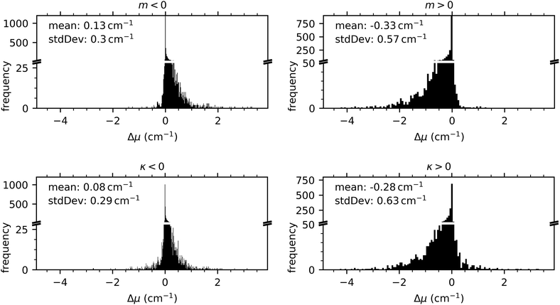
Fig. 5 shows four histograms for negative and positive gradients and curvatures. The histograms show a positive shift of the line position for negative gradients with a mean value of 0.13 cm⁻¹ and a negative shift for positive gradients with a mean value of −0.33 cm⁻¹. On a negatively curved background, the rolling circle filter similarly induces a positive shift of the line position of 0.08 cm⁻¹ on average and a negative shift with a mean value of −0.28 cm⁻¹ for positively curved backgrounds. To translate this to an uncertainty contribution to the line position induced by the rolling circle filter, we calculated 68% and 95% intervals of the histograms shown in Fig. 5. These intervals, serving as a measure for this uncertainty contribution, together with the symmetrical standard deviation of the distributions are shown in Table 4.

Fig. 5 Statistical distribution of the difference of the peak positions Δμ before and after filtering with the rolling circle filter for different intervals of the gradient m and curvature κ. The broken y-axis is only used to make the flanks of the distribution visible, and no data are left out in between.

Table 4 Results of the statistical analysis of the difference in the peak position before and after filtering with the rolling circle filter giving the mean μ, standard deviation (std. dev.), and 68% and 95% intervals of the statistical distributions

Criteria	Δμ (cm^−1)	std. dev. (cm^−1)	68% interval (cm^−1)		95% interval (cm^−1)
m > 0	−0.33	0.57	−0.90	0.24	−1.45	0.80
m < 0	0.13	0.30	−0.17	0.43	−0.46	0.72
κ > 0	−0.28	0.63	−0.91	0.35	−1.52	0.96
κ < 0	0.08	0.29	−0.20	0.37	−0.48	0.65

---

3.3.2 Peak width and intensity. To quantify the influence of the rolling circle filter on the peak width and intensity, we selected two intervals for each of the parameters width σ, intensity I, slope m and curvature κ. These intervals are given in Table 5. To cover a large parameter space, but reduce the scattering of the data points, the data are filtered by fixing all but one parameter in the first interval and setting this selected parameter to its second interval. This procedure leads to two significant correlations: the difference Δσ = σ − σ_f of the width (see Fig. 6) and the difference ΔI = I − I_f of the intensity (see Fig. 7) before and after filtering correlate with the width after filtering σ_f. This is an expected behavior, since the rolling circle filter rolls into the peaks and the area that is thereby subtracted from the lines depends on the line width. This effect therefore reduces the line intensity, and also the line width. We quantified this effect by a regression of the function

y(σ) = a·σ² + b·σ³. (2)

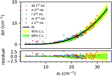Fig. 6 Correlation of the width difference Δσ and width after filtering σ_f. The data are selected according to the intervals given in Table 5. First, the data with all parameters in the first interval (all 1^st int.) are shown. Then, only one parameter is switched to its second interval, and these data are labelled with the corresponding parameter and ‘2^nd int.’. The solid line shows the fit of eqn (2) with the resulting confidence intervals.

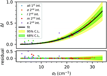Fig. 7 Correlation of the intensity difference ΔI and width after filtering σ_f. The data are selected according to the intervals given in Table 5. First, the data with all parameters in the first interval (all 1^st int.) are shown. Then, only one parameter is switched to its second interval, and these data are labelled with the corresponding parameter and ‘2^nd int.’. The solid line shows the fit of eqn (2) with the resulting confidence intervals.

Table 5 Parameter ranges for peak selection

Parameter	1^st interval		2^nd interval
	Min	Max	Min	Max
σ	5	25	25	50
I	0.3	0.6	0.6	1.0
m	−5 × 10^−5	0	0	5 × 10^−5
κ	−5 × 10^−7	0	0	5 × 10^−7

---

The results of this regression, suitable for quantification and correction of the systematic uncertainty induced by the rolling circle filter, are shown in Table 6.

Table 6 Polynomial regression of the parameter correlations

y([small nu, Greek, tilde])	a	b	red. χ^2
ΔI	9.3 ± 4 × 10^−5	1.7 ± 0.2 × 10^−5	6.8 × 10^−3
Δσ	−4.3 ± 0.5 × 10^−3	5.6 ± 0.2 × 10^−4	6.1 × 10^−2

---

3.4 Discussion

The simulation showed that the rolling circle filter influences the position of a spectral line, depending on the curvature and gradient of the underlying baseline. We quantified this shift to approximately −0.3 cm⁻¹ for positive and 0.1 cm⁻¹ for negative gradients and curvatures. The systematic uncertainties of this shift can be quantified via 68% confidence intervals, see Table 4, and are below 1 cm⁻¹. Therefore, this influence in the sub-wavenumber region is only relevant for highly precise spectroscopic investigations. Since this shift is smaller for narrower peaks, we can conclude that the rolling circle filter in combination with peak fitting does not enable high precision measurements on broad spectral lines.

Regarding the peak width and intensity, there is a strong influence of the rolling circle filter, causing broad peaks to vanish completely after the filtering. Using the parametrizations of the systematic effect of the rolling circle filter on the peak intensity and width, it is possible to quantify this effect as a systematic uncertainty and the parametrization can be used to correct it for further analysis. This intensity correction makes the rolling circle filter suitable for investigation of the intensities of spectral lines as it is for line positions.

4. Conclusion

We have shown that the filter optimization procedure is necessary to prevent a detachment of the baseline, while minimizing the distortion of the spectral lines by the filter. Our method then enables a quantification of the remaining influence of the filter regarding real spectra, that occurs, as the filter can only be optimized to a certain line width, intensity and background curvature. We quantify the influence of the filter on these varying parameters by the subsequent systematics study. This combined method leads to a filter procedure that delivers a reliable baseline with a known and therefore correctable influence on the spectral shape.

In our case, line intensities are used for concentration measurement, and this is a crucial result on the way to a calibration that is independent of the instrument used. A transfer of the calibration results to a different experimental setup is only possible if the systematic influences of the respective instrument and analysis procedure are known and can be corrected, if significant. Also, if the measurement samples significantly differ from the calibration samples, the performed quantification and correction of the systematic effects of the filter is the only possibility to obtain reliable measurement values in such a setting. Both issues can be solved with the presented combination of filter optimization and residual systematic uncertainty quantification.

The method can, with small modifications, be applied to different filters, since filters for baseline approximation should always provide a smooth baseline without extreme curvatures or even edges. Under these conditions, χ² should be a suitable measure for the quality of the baseline approximation. Furthermore, the creation of a filter bank with different filter settings, e.g. radii of the rolling circle filter, for different spectral regions can be a promising content of further studies. This can deliver a significant advantage compared to a single filter setting, in the case of strongly varying line widths or background curvature. The presented method for the optimization of the rolling-circle-filter and the quantification of the remaining systematic effects on the peak shape can be the basis for a study that optimizes and compares different filter methods, such as rolling circle, averaging, wavelet and derivative filters. While such a systematic comparison and evaluation is beyond the scope of the presented work, we will address this in a future publication on this topic.

Conflicts of interest

There are no conflicts to declare.

References

1. D. K. Veirs and G. M. Rosenblatt, J. Mol. Spectrosc., 1987, 121, 401–419.
2. M. Schlösser, B. Bornschein, S. Fischer, T. M. James, F. Kassel, S. Rupp, M. Sturm and H. H. Telle, Fusion Sci. Technol., 2015, 67, 555–558.
3. R. Größle, A. Beck, B. Bornschein, S. Fischer, A. Kraus, S. Mirz and S. Rupp, Fusion Sci. Technol., 2015, 67, 357–360.
4. R. Größle, A. Kraus, S. Mirz and S. Wozniewski, Fusion Sci. Technol., 2017, 71, 369–374.
5. H. G. Schulze, A. Jirasek, M. M. L. Yu, A. Lim, R. F. B. Turner and M. W. Blades, Appl. Spectrosc., 2005, 59, 545–574.
6. H. G. Schulze, R. B. Foist, K. Okuda, A. Ivanov and R. F. B. Turner, Appl. Spectrosc., 2012, 66, 757–764.
7. C. Rowlands and S. Elliott, J. Raman Spectrosc., 2011, 42, 363–369.
8. A. Savitzky and M. J. E. Golay, Anal. Chem., 1964, 36, 1627–1639.
9. I. K. Mikhailyuk and A. P. Razzhivin, Instrum. Exp. Tech., 2003, 46, 765–769.
10. Y. Y. Huang, C. M. Beal, W. W. Cai, R. S. Ruoff and E. M. Terentjev, Biotechnol. Bioeng., 2010, 105, 889–898.
11. S.-K. Oh, S. J. Yoo, D. H. Jeong and J. M. Lee, Bioresour. Technol., 2013, 142, 131–137.
12. E. U. Donev, J. I. Ziegler, R. F. H. Jr and L. C. Feldman, J. Opt. A: Pure Appl. Opt., 2009, 11, 125002.
13. T. M. James, M. Schlösser, R. J. Lewis, S. Fischer, B. Bornschein and H. H. Telle, Appl. Spectrosc., 2013, 67, 949–959.
14. S. Mirz, U. Besserer, B. Bornschein, R. Größle, B. Krasch and S. Welte, Fusion Sci. Technol., 2017, 71, 375–380.
15. N. N. Brandt, O. O. Brovko, A. Y. Chikishev and O. D. Paraschuk, Appl. Spectrosc., 2006, 60, 288–293.
16. I. N. Bronstein, K. A. Semedjajew, G. Musiol and H. Mühlig, Taschenbuch der Mathematik, Verlag Harri Deutsch, 6th edn, 2006.
17. C. Runge, Math. Ann., 1895, 46, 167–178.
18. K. Levenberg, Q. Appl. Math., 1944, 2, 164–168.
19. K. Levenberg, SIAM J. Appl. Math., 1963, 11, 431–441.

---