
 Open Access Article
 This Open Access Article is licensed under a
 Creative Commons Attribution 3.0 Unported Licence
Studying polymer solutions with particle-based models linked to classical density functionals: co-non-solvency
Jianguo
Zhang
,
Debashish
Mukherji
 ,
Kurt
Kremer
* and
Kostas Ch.
Daoulas
*
,
Kurt
Kremer
* and
Kostas Ch.
Daoulas
*
Max Planck Institute for Polymer Research, Ackermannweg 10, 55128 Mainz, Germany. E-mail: kremer@mpip-mainz.mpg.de; daoulas@mpip-mainz.mpg.de
First published on 30th October 2018
Abstract
We demonstrate the potential of hybrid particle-based models, where interactions are introduced through functionals of local order parameters, in describing multicomponent polymer solutions. The link to a free-energy-like functional is advantageous for controlling the thermodynamics of the model. We focus on co-non-solvency – the collapse of polymer chains in dilute mixtures with two miscible good solvents, having different affinities towards the polymer. We employ a simple model where polymers and solvents are represented, respectively, by worm-like chains and single particles. Non-bonded interactions are captured by a polynomial which is third order in local densities and can, therefore, describe liquid–vapour coexistence. The parameterisation of the functional benefits from an elementary mean-field approximation to the statistical mechanics of the model. The model provides a framework for Monte Carlo simulations using a particle-to-mesh algorithm. Studies with conventional generic bead-spring and all-atom models have demonstrated that co-non-solvency is caused by preferential binding of the better solvent (termed cosolvent) with polymer. Hence, segmental loops bridged by cosolvent molecules are formed, initiating polymer collapse. The mesoscopic hybrid model differs conceptually from the conventional microscopic descriptions. Yet, it reproduces the same co-non-solvency mechanism supporting its universality. Films of adsorbed ternary solutions, showing co-non-solvency in the dilute regime, are considered at high concentrations. In this case, chains do not collapse. The properties of loops and tails of the adsorbed polymer agree with early theoretical predictions obtained for concentrated binary solutions.
1 Introduction
Many fundamental studies and technological applications of soft matter involve polymers mixed with several solvents. To understand theoretically complex interrelationships1 between structure, processing, and properties of multicomponent polymer solutions, molecular simulations are commonly required. These interrelationships often involve length and time scales which can be addressed only using mesoscopic descriptions: molecular models where large groups of actual chemical units are mapped on a single effective particle. Drastic coarse-graining reduces significantly the degrees of freedom and softens the interactions, making them comparable to the thermal energy. Therefore the computational time remains tractable. The difficulty in defining the mesoscopic interactions is one of the downsides of drastic coarse-graining. Standard bottom-up strategies2,3 require reference data from computationally expensive simulations based on detailed models. Moreover, performing reference simulations of polymer solutions with new and complex formulations,4–6 often requires adjustments of existing atomistic force fields. Finally, bottom-up strategies suffer from state-point and representability dependent parameterisation.Top-down coarse-graining of polymer solutions is an alternative strategy where mesoscopic models are developed postulatively, aiming to reproduce by construction a set of known properties. Based on this pre-existing (limited) knowledge, top-down modelling can interpret and predict other features.3 Thermodynamic properties of fluids play a key role in chemical engineering,7–9 are extensively documented, and can provide guidelines for top-down modelling. Constructing and improving force fields using thermodynamic information is a common practice in atomistic and moderately coarse-grained (CG) models; the NERD10 and MARTINI11 force fields are typical examples.
Top-down particle-based models linked to continuum free-energy-based descriptions allow one to introduce systematically12–14 thermodynamic information. These approaches describe the molecular architecture of different compounds similarly to standard CG models. However, non-bonded interactions are templated by functionals15–20 of local order parameters. Structurally, these functionals are similar to free energies in classical density functional theory (DFT) and phase-field models. Yet, they are conceptually different because they depend on instantaneous order-parameter fields (and not average). The functionals are transformed into mesoscopic force fields by expressing the instantaneous local order parameters through the coordinates of the CG particles. The hybrid method simplifies the construction of particle-based models with desired thermodynamics, because the thermodynamic properties are already determined by the templating functional. Simple mean field (MF) estimates, Self Consistent Field (SCF) theory, and classical DFT facilitate the choice of a functional suitable for reproducing the target thermodynamic behaviour. Importantly, introducing interactions through functionals of fields of local order parameters facilitates coupling with other continuum techniques. For example, hybrid schemes combining21–23 dynamic SCF theory (based on quadratic density functionals) with the Lattice Boltzmann method have been used to explore the effect of hydrodynamic interactions on the kinetics of self-assembly in block-copolymer-based solutions.22,23
Although the popularity of hybrid models in modelling Soft Matter is increasing,12–14,24 their potential in modelling polymer solutions has not yet been fully explored. Currently, hybrid models of polymer solutions22,23,25–34 are build on functionals which are polynomials of local densities of different compounds. Most studies focus on phenomena in the liquid phase (such as self-assembly) and retain only second-order terms, which are equivalent to simple Flory–Huggins interactions. Significantly less studies incorporate polynomials of higher order, which are necessary to cover a broader range of phase behaviour.27,35 For example, using third-order density polynomials is the minimum requirement to have coexisting liquid and vapour phases. The few studies with higher order functionals usually consider the solvent implicitly. Namely, the “vapour” phase is actually an integrated-out phase12,25,26,28,29 of liquid solvent at equilibrium with an explicitly described polymer-rich phase. A single solvent component and an actual vapour phase have been introduced only in a very limited number of studies to describe processes in films of polymer solutions, such as drying27 and solvent annealing.32
Here we expand previous studies and investigate whether simple mesoscopic hybrid models can capture complex phenomena sensitive to the formulation of multicomponent polymer solutions. We focus on the phenomenon of co-non-solvency, which occurs when a polymer collapses in mixtures of two competing miscible good solvents. This phenomenon has been extensively studied in various experimental setups.36–44 From the simulation side a rather limited number of studies has been performed to understand this puzzling phenomenon, including chemical-specific40,45,46 and generic simulations.47–50 We note that in some of these studies48 at least one of the solvents was described implicitly, in a mean-field manner. Co-non-solvency has also been addressed in a number of works based on analytical theories.36,49–54 In previous works, two of us have demonstrated that the collapse of the chain is driven by preferential binding of the better solvent in the pair (named in the following cosolvent) with polymer monomers.49,50 The aggregation of cosolvent molecules onto the chains facilitates the formation of enthalpically favourable segmental loops. The process leads to the formation of a compact globule. This observation of preferential binding is also closely complemented by NMR and AFM experiments.41,44 Co-non-solvency depends49 on the local structure of the liquid (i.e. energy density within the solvation shell). In hybrid models soft CG units overlap, there are many interacting neighbours, and the liquid structure is captured only on mesoscopic level.18 Furthermore, local liquid packing is affected by the specific method used to calculate13 the interactions, e.g. particle-to-mesh (PM) schemes15,18,28,55,56 or density distributions.15–17,19,20 Due to these simplifications, it is not known beforehand whether hybrid models reproduce co-non-solvency and, if so, which features.
First we demonstrate that co-non-solvency can be indeed reproduced by hybrid models constructed using basic thermodynamic reasoning. We intentionally implement a simple hybrid model of ternary solutions which (i) describes explicitly the three components (polymer, solvent, and cosolvent), (ii) is based on third-order density polynomials, and (iii) is combined with a rudimentary PM scheme for calculating interactions. The modelling approach captures qualitatively most of the known features of co-non-solvency. Subsequently, we use this model to describe the same ternary solutions, coated on a solid substrate in the concentrated regime. In these films, we explore the properties of adsorbed layer and compare them with analytical predictions known from simple binary solutions.
2 Modelling concept
The modelling approach can be formalised through the canonical configurational partition function: | (1) |
The index a indicates the component type and na denotes the number of molecules of each component. The coordinates of the s-th monomer in the i-th molecule are defined by ri(s) and Na is the total number of monomers in a molecule of component a. In this work, the three components are defined by a = p (polymer), s (solvent), and c (cosolvent). The integral  is taken over the possible realisations of the coordinates of all monomers. The ansatz is general enough to allow the description of branch-like polymers and solvents which are composed of several monomers, i.e. are chain-like. The architecture of molecules of component a is described by the effective Hamiltonian of bonded interactions, Hb(a). The effective Hamiltonian of non-bonded interactions, βHnb, is expressed through a functional, f, of local densities,
 ![[small rho, Greek, circumflex]](https://www.rsc.org/images/entities/i_char_e0b7.gif) a(r), of monomers belonging to the different components. In our study, we assume in eqn (1) that the molecules of each component are comprised of monomers of a single chemical species, e.g. polymers are homopolymers. Generalising to molecules with chemically different monomers is straightforward. The functional f depends on instantaneous values of densities (indicated by the “hat”). Essentially, a(r) are operators transforming a configuration of particle coordinates, R, into instantaneous fields of collective variables. To define the model, in addition to Hb(a) and βHnb, the density operators must be specified.
a(r), of monomers belonging to the different components. In our study, we assume in eqn (1) that the molecules of each component are comprised of monomers of a single chemical species, e.g. polymers are homopolymers. Generalising to molecules with chemically different monomers is straightforward. The functional f depends on instantaneous values of densities (indicated by the “hat”). Essentially, a(r) are operators transforming a configuration of particle coordinates, R, into instantaneous fields of collective variables. To define the model, in addition to Hb(a) and βHnb, the density operators must be specified.
3 Simple model for ternary solutions
In this section we describe a simple hybrid model for ternary mixtures. Though generic, the model is parameterised such that some thermodynamic properties are qualitatively similar to actual materials.3.1 Particle-based description
Polymers are described using the discrete worm-like chain (WLC) model, also termed57 as “elastically-jointed chain”. Each chain has Np “monomers” placed at the ends and junctions of the WLC or, equivalently, Np − 1 segments with fixed length b. The bonded interactions are defined through the Hamiltonian: | (2) |
 | (3) |
This equation follows from a well-known relationship57 between the persistence length lp and ε, considering that lk = 2lp when ε ≫ 1.
Solvent and cosolvent molecules are represented by single beads, so that Ns and Nc equal unity. Therefore there are no bonded interactions associated with these two species.
3.2 Non-bonded interactions
We define non-bonded interactions through a third-order polynomial of local densities: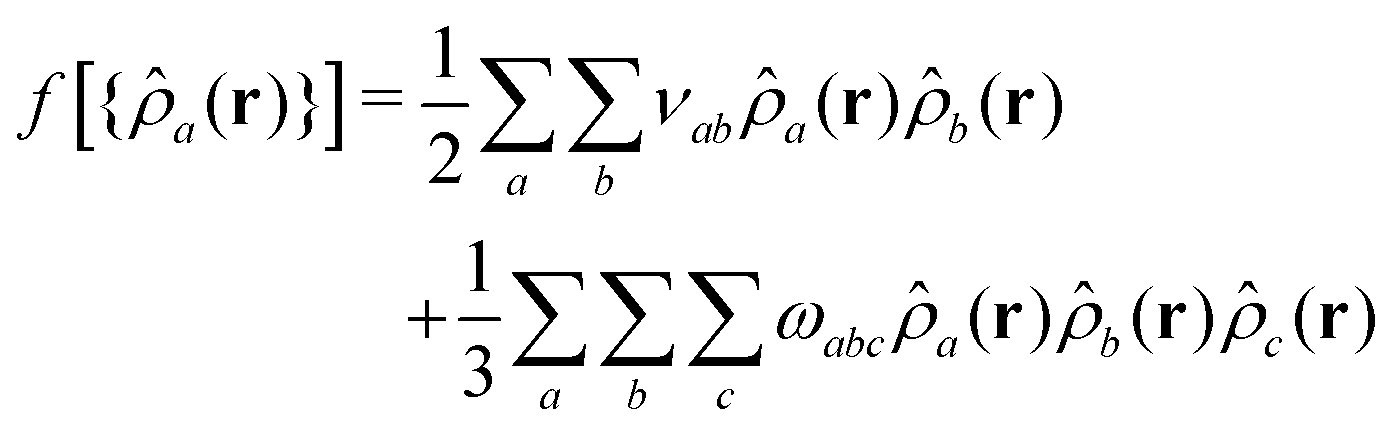 | (4) |
When required, interactions with the substrate are described using the generic potential:60
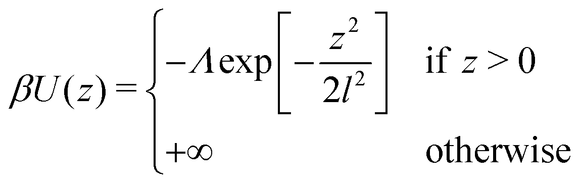 | (5) |
3.3 Simulation method
The hybrid model provides a framework for Monte Carlo (MC) simulations. We use the canonical ensemble and place the solutions into a simulation box with edges Lγ, γ = x, y, z. The length of Lγ as well as the amount of polymer, solvent, and cosolvent molecules in the box, are specific to the studied system and will be discussed during the presentation of results in Section 4. Bulk solutions are modelled with periodic boundary conditions (PBC) in all three directions. When modelling films, there are no PBC along z-direction: the box is sealed at z = 0 and Lz with the potential βU(z) and an enthalpically neutral hard wall, respectively.A MC algorithm requires the calculation of energies from particle coordinates. Calculating the bonded energy and the energy from interactions with the substrate is straightforward by direct substitution of coordinates into eqn (2) and (5). However, the calculation of non-bonded interactions requires instantaneous fields of densities. We obtain these densities from the coordinates of the particles, distributed in continuum space, through a PM scheme. The simulation box is discretised through a cubic lattice with cell-size ΔL. The densities a(c) at a grid-node, with coordinates c, are calculated from:
 | (6) |
The integral defining Hnb is discretised into a sum over the Ncell nodes of the lattice, substituting  . After this step, MC sampling becomes straightforward. To sample the conformations of WLC we employ two standard algorithms: the slithering snake62,63 (reptation) and the crankshaft64 move, termed sometimes65 “flip”. During the reptation move, a chain is randomly selected. One segment is removed from a randomly chosen end of the chain and attached to the opposite end. We use the simplest version of the reptation algorithm, where the new orientation of the segment is selected randomly without bias. Since only one segment is involved, each reptation move can propagate the chain by maximum one bond length b. The rotation angle65 in the crankshaft (flip) move is chosen randomly from the interval [−π,π]. For solvent and cosolvent molecules we use small random displacements: each of the three Cartesian coordinates of the displacement vector is randomly chosen from the interval [−Δl,Δl], where Δl = lk/5. Since these displacements were sufficient for the purposes of our study, we did not attempt to optimise sampling, e.g. by considering larger Δl. The new density ρnewa(c) in the cells affected by the MC move is calculated considering the coordinates of the displaced particles of species a at their proposed and old positions. Taking into account, the old density ρolda(c) in the same cells, the difference in the nonbonded energy ΔHnb is obtained. Depending on the particle species changes of energy due to bonded interactions and substrate potential (when present) are calculated, as well. After all changes in energy are available, the Metropolis acceptance criterion is applied. In films (no PBC along z direction) the MC move is rejected straightaway if the displaced monomer, solvent, or cosolvent particles are found outside the boundaries of the box.
The lattice spacing sets the range of interactions and is a key parameter in PM schemes.18,61 We choose ΔL comparable to the length of the Kuhn segment, which is the fundamental length scale of our model, setting ΔL = 1.05.
3.4 Parameterisation strategy
To define βHb(p) we set the stiffness of the WLC to ε = 2.99 which, according to eqn (3), leads to lk/b ≃ 5. This empirical choice ensures that the number of particles per lattice cell in the liquid phase is on the order of 20 (cf. data provided further in the text). Because of this rather large number of interacting neighbours, the behaviour of the model in the liquid phase can be qualitatively estimated through elementary MF and the coefficients of the polynomial f follow from simple physical arguments.Rudimentary MF approximation to the full statistical-mechanical description of the hybrid model given by eqn (1), leads to a Helmholtz free energy of homogeneous phases:27
 | (7) |
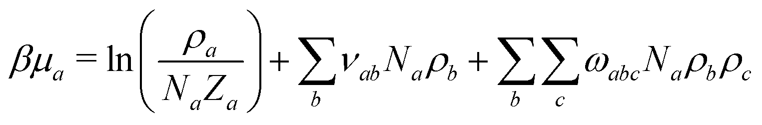
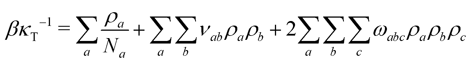
![[small rho, Greek, macron]](https://www.rsc.org/images/entities/i_char_e0d1.gif) a(l). The first term in eqn (7) is the entropic part, where Za represents the single-molecule partition function of each component. Similarly to the standard Flory–Huggins model, this MF treatment assumes that Za do not depend on composition. Hence, only translational entropy is present. From the simple Helmholtz free energy one can estimate observables such as pressure, P = −∂F/∂V, chemical potentials, μa = ∂F/∂na, and response functions, e.g. isothermal compressibility, 1/κT = −V∂P/∂V.
a(l). The first term in eqn (7) is the entropic part, where Za represents the single-molecule partition function of each component. Similarly to the standard Flory–Huggins model, this MF treatment assumes that Za do not depend on composition. Hence, only translational entropy is present. From the simple Helmholtz free energy one can estimate observables such as pressure, P = −∂F/∂V, chemical potentials, μa = ∂F/∂na, and response functions, e.g. isothermal compressibility, 1/κT = −V∂P/∂V.
To parameterise f we use the observables:
 | (8) |
 | (9) |
 | (10) |
We first determine νaa and ωaaa controlling the thermodynamics of pure components. For this purpose, we consider liquid/vapor phase equilibrium in pure polymer, solvent, and cosolvent, fixing a priori the density and the compressibility of the liquid phase. We postulate that the density of WLC monomers p(l) in the pure polymer liquid should be representative of classical polymer melts. It is convenient to express the monomer density as p(l) ≃ (lk/b)no, where no is the number of Kuhn segments found in the characteristic volume lk3. The quantity no is a well known material parameter, which is related to rheological properties66 and is often written equivalently as lk/p (p is the packing length). For many polymers66 1 ≤ no ≤ 10 and we choose no = 4.17, which corresponds to a standard polymer – atactic PMMA. For lk/b = 5, the number density of monomers in the polymer liquid is p(l) = 20.85. Because our study is generic, we assume that solvent and cosolvent have different interactions with the polymer but are identical with respect to all other properties. Moreover, this simple choice guarantees that solvent and cosolvent are miscible in the entire range of molar compositions, which is the typical for solvent mixtures where co-non-solvency is observed.36,50 For simplicity we also assume that the number density of particles in the liquid phases of pure solvent and pure cosolvent is the same as for the polymer. That is, we set s(l) = c(l) = (l), where (l) = 20.85. Hereafter we set T = 400 K, which is representative of temperatures where polymers are found in molten state.
Liquids are characterised by low compressibilities, i.e. typically κT ∼ 10−9–10−10 Pa−1. However, hybrid models with small compressibility pose significant challenges to PM schemes. The intrinsic width of the interface of a polymer liquid (melt or solution) with its vapor is on the order of the Edwards correlation length ξ. In melts the Edwards correlation length67–69ξm, is given by  while in solutions
 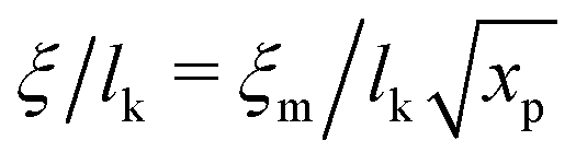 . Here xp is the volume fraction of polymer segments. Using these expressions it is straightforward to estimate that κT ∼ 10−9 Pa−1 leads to ξ ∼ 10−2 × lk. Therefore, realistic compressibilities lead to interfaces which are significantly narrower than ΔL and lattice-related artefacts are expected. To broaden the interfaces, we use for liquid polymer, solvent, and cosolvent κT = 10−8 Pa−1. Increasing the compressibility by an order of magnitude mitigates lattice-related artefacts, while the density contrast between vapor and liquid phases remains high (cf. discussion in Section 3.5).
Using p(l) and κT as an input, νaa and ωaaa are estimated from the single-component limit of eqn (8)–(10). The calculations for the polymer are simplified considering that the pressure in polymer melts at equilibrium with their vapor is negligibly small and can be therefore approximated by zero.70 Substituting P = 0 and ρp = p(l), eqn (8) and (10) are solved with respect to νpp and ωppp. For the solvent and the cosolvent the vapor pressure is not known and the complete condition of phase equilibrium is required, given by P((l)) = P(ρsata(v)), μ((l)) = μ(ρsata(v)), and κT−1((l)) = κT−1. Unknowns in these equations are νaa, ωaaa, and the saturation density of the vapor phase ρsata(v) (here a = s or c). The parameters νaa and ωaaa obtained from the solution of the equations are listed in Table 1, while ρsata(v) ≃ 0.5.
| Parameters | Values | Parameters | Values |
|---|---|---|---|
| ν pp | −0.291745 | ω sss | 0.0135882 |
| ν ss | −0.474503 | ω ccc | 0.0135882 |
| ν cc | −0.474503 | ω pps | 0.0111569 |
| ν ps | −0.36508 | ω pss | 0.0122297 |
| ν sc | −0.474503 | ω ssc | 0.0135882 |
| ν pc | −0.84 | ω scc | 0.0135882 |
| ω ppp | 0.0103696 | ω pcc | 0.0197092 |
| ω ppc | 0.0186364 | ω psc | 0.0124173 |
Next we specify the parameters determining polymer–solvent and polymer–cosolvent interactions: νpa, ωpaa, and ωppa. The coefficient νpa plays a key role in controlling the affinity of the solvent (cosolvent) to the polymer. The value νps = −0.36508 used to reproduce good solvent conditions is included in Table 1. This choice is based on trial simulations exploring the parameter space around νpa = (νpp + νaa)/2. At this reference point, the Flory–Huggins parameter χ, to a first approximation,12 equals zero, i.e. good solvent conditions are guaranteed. We note that this approximation neglects effects of composition on χ from the third-order density terms in f. A more rigorous treatment of composition effects on χ can be found elsewhere.32,70 In general, the isothermal compressibility κT obtained viaeqn (10) will depend on composition. We reduce the dependency of κT on composition by suitable choice of ωpss and ωpps. Details are provided in the Appendix.
Because the solubility of polymer in cosolvent is higher than in solvent, νpc < νps. The magnitude of νpc required to observe co-non-solvency can be estimated45,49 from ternary mixtures of disconnected polymer monomers, solvent, and cosolvent particles. At infinite dilution, ρp → 0, the excess chemical potential of monomers follows from eqn (9) as a function of composition of the mixture:
| βμp(ex)(xc) = νps(l)(1 − xc) + νpc(l)xc + ωpss(l)2(1 − xc)2 + 2ωpsc(l)2(1 − xc)xc + ωpcc(l)2xc2 | (11) |
The composition is described via the volume fraction of the cosolvent xc = ρc/(l). Based on eqn (11) we define a difference of excess chemical potentials Δμp(ex)(xc) = μp(ex)(xc) − μp(ex)(0). Observations in conventional particle-based simulations empirically suggest45,49 that co-non-solvency occurs first when Δμp(ex)(1) is somewhere between −2 and −4kT. Setting νpc = −0.84 leads to Δμp(ex)(1) ≃ −6.8kT which, as will be demonstrated in Section 4.1, reproduces co-non-solvency. Note that for each choice of νpc the parameters ωpcc and ωppc are determined as in the case of solvent, i.e. they cancel the dependency of κT on composition. Table 1 lists these parameters for νpc = −0.84.
Because solvent and cosolvent particles are identical to each other (except from their interactions with the polymer) we set ωssc = ωscc = ωsss = ωccc. The single parameter related to simultaneous interactions of the three different species is determined via the combination rule 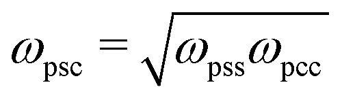 .
.
Regarding the interactions with the substrate, we set for solvent and cosolvent particles Λ = 0. For the interactions between the monomers and the substrate we employ Λ = 0.32 and l = 0.6. With this choice, the adsorption energy per unit area is estimated (roughly) to 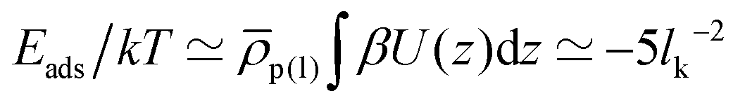 . For a typical Kuhn segment length lk = 1.5 nm, this estimate leads to Eads/kT ≃ −2.1 nm−2 which is comparable to magnitudes reported for actual materials.60,71,72
3.5 Limitations of the generic hybrid model
We expect straightaway that the hybrid model introduced in the previous sections has a number of limitations.While the generic third-order density polynomial in eqn (4) is sufficient for our qualitative study, it is too simple to reproduce accurately the thermodynamics of most real systems, e.g. their equations-of-state. Such limitations have been discussed, for example, when modelling35 alkane oligomers mixed with CO2 or water on corrugated substrates.73 Various more complex free-energy models are available and are a basic tool for describing the thermodynamics of actual materials.74 Applying density functionals based on these models in hybrid modelling has significant potential but remains largely unexplored. For instance, the Sanchez–Lacombe equation-of-state has been only recently applied in hybrid modelling of homopolymer melts.75 In the past, third-order density polynomials have been applied70 to systems forming hydrogen bonds. In this case they are analogous to Flory–Huggins models with negative Flory–Huggins parameters. A fundamental restriction of this approach is that it cannot capture the saturation of hydrogen bonds.76 This problem can be addressed using association models that introduce hydrogen bonding as an explicit reaction between particles. MF treatments of association models allow the formulation of free energies of systems with hydrogen bonds.76–78 In this case, the determination of the free-energy part which is related to the association of the particles presents a difficult combinatorial problem. This complication is avoided in hybrid simulations because they operate with ensembles of multiple, correlated chains. Therefore, it is possible79 to describe association introducing reversible bonds between particles, e.g. through appropriate MC moves, similarly to standard particle-based simulations of equilibrium polymers.80
The parameters of the model are determined to satisfy MF equations linking them to thermodynamic observables used as an input. MF-based parameterisation is straightforward but does not allow one to completely control the thermodynamic properties of the hybrid model. The reason is that hybrid simulations incorporate fluctuations and correlation effects which MF neglects. Therefore, for a given set of parameters, the thermodynamic properties in hybrid simulations usually differ from their MF counterparts. Such deviations will be reported in Section 4. Therefore, the parameters of our model are reported in Table 1 with high accuracy only to facilitate the reproducibility of calculations discussed in Section 3.4. In practice, to obtain a hybrid model with qualitatively predictable thermodynamics, parameters (as those presented in Table 1) can be truncated – the MF-based parameterisation is anyway approximate. A simple rule of a thumb is to truncate the parameters such that after back-insertion into MF equations they reproduce the target quantities, e.g. densities, with an accuracy 0.1%.
As has been discussed in Section 3.4, making the liquid more compressible (increasing κT) mitigates artefacts such as pinning of interfaces to the lattice. While this ansatz is sufficient for our generic qualitative study, we expect that reproducing actual vapour/liquid equilibria (VLE) of polymer solutions will require models with smaller κT. To identify the interdependence of compressibility and VLE, let us assume that the densities of the liquid and vapor phases of a pure solvent s(l) and ρsats(v), that are at equilibrium with each other at given temperature, are experimentally known. The coefficients νss and ωsss, necessary to reproduce this VLE point with a third-order density functional, are obtained by solving the set of two linear equations P(s(l)) = P(ρsats(v)) and μ(s(l)) = μ(ρsats(v)) (in this case νss and ωsss are the unknowns, cf.eqn (8) and (9)). Substituting these coefficients into eqn (10) delivers, within the model of a third-order density functional, the relationship between compressibility and density contrast of liquid and vapor phases:
 | (12) |
s(l). Based on eqn (12), we illustrate how realistic VLE data can lead to low κT considering acetone as an example. For this standard organic solvent, two representative VLE points obtained81 from atomistic simulations (based on the OPLS force-field) are: (i) MWss(l) ≃ 778![[thin space (1/6-em)]](https://www.rsc.org/images/entities/char_2009.gif) kg m−3 and MWsρsats(v) ≃ 1.46kg m−3 at T = 300 K, and (ii) MWss(l) ≃ 657 kg m−3 and MWsρsats(v) ≃ 18.2 kg m−3 at T = 400 K. MWs ≃ 0.058 kg mol−1 stands for the molecular weight of the acetone (in contrast to the other parts of our paper, in the example for the acetone the number densities are expressed in mol m−3 for consistency with ref. 81). Eqn (12) delivers for these two VLE points κT ≃ 4 × 10⁻⁹ and 9 × 10⁻⁹ Pa−1, respectively. Liquids with κT ∼ 10−9 can be modelled82 by combining density functionals with density distributions defined in continuum space, which avoids a PM discretisation. Multibody Dissipative Particle Dynamics16,17,83 is an example of such strategies.
kg m−3 and MWsρsats(v) ≃ 1.46kg m−3 at T = 300 K, and (ii) MWss(l) ≃ 657 kg m−3 and MWsρsats(v) ≃ 18.2 kg m−3 at T = 400 K. MWs ≃ 0.058 kg mol−1 stands for the molecular weight of the acetone (in contrast to the other parts of our paper, in the example for the acetone the number densities are expressed in mol m−3 for consistency with ref. 81). Eqn (12) delivers for these two VLE points κT ≃ 4 × 10⁻⁹ and 9 × 10⁻⁹ Pa−1, respectively. Liquids with κT ∼ 10−9 can be modelled82 by combining density functionals with density distributions defined in continuum space, which avoids a PM discretisation. Multibody Dissipative Particle Dynamics16,17,83 is an example of such strategies.
4 Results and discussion
4.1 Bulk solutions
Before modelling co-non-solvency in ternary systems, we verify that our model reproduces characteristic behaviour of polymer solutions in single good solvent. We start from the dilute regime performing canonical MC simulations in cubic boxes with edge length L, containing ns solvent particles and a single polymer chain with Np = 661 (equivalent to 132 Kuhn segments). To model dilute bulk solutions, the total density in the box, ρ0, must be sufficiently high to exclude coexisting liquid and vapor phases. A first choice is to set ρ0 equal to the liquid density,s(l), used for the MF parameterisation of βHnb. However, as has been discussed in Section 3.5 the thermodynamics in the particle-based simulations differs from the approximate MF solution. Therefore setting ρ0 = s(l) leads to the formation of small vapor “bubbles” motivating us to work with somewhat higher densities, ρ0 ≃ 22.56. Fig. 1 presents the log–log plot of the polymer structure factor, S(q), calculated from simulations in the dilute regime. The intermediate q range follows the scaling S(q) ∼ q−5/3 (blue line), as expected for polymer chains in good solvent (dilute regime). At larger q, S(q) ∼ q−1 (red line), manifesting the rod-like behavior of the chain on length scales comparable to the Kuhn segment. For these simulations we set L = 23, which is more than three times larger than the radius of gyration, Rg(0) ≃ 6.5, of the polymer in the dilute solution.
 | ||
| Fig. 1 Single-chain structure factor, S(q), for a WLC polymer with Np = 661 monomers in a dilute mixture with solvent. The universal scaling laws S(q) ∼ q−5/3 and q−1 expected for wavevectors probing (respectively) the length scales of the self-similar structure of the coil and the Kuhn segment are shown with blue and red lines. | ||
We increase gradually the concentration replacing solvent particles by polymer chains containing an equivalent amount of monomers. This procedure preserves the total number density fixed to ρ0 ≃ 22.56. The main panel of Fig. 2 presents the average gyration radius Rg as a function of polymer volume fraction xp (the average monomer number density normalised by ρ0). As expected for polymers in good solvent, Rg becomes smaller as xp increases and converges to the value for the melt (xp = 1). We compare our results with the scaling law84Rg/Rg(0)= (xp/xp*)−f in the inset of Fig. 2. The overlap concentration is defined as xp* = 3Np/4π(Rg(0))3ρ0, and f = (2νeff − 1)/(6νeff − 2). The scaling exponent νeff = 0.56, obtained by fitting the data for concentrations 1 < xp/xp* < 10, is not that far (∼5% smaller) from the theoretically expected νeff = 0.588. The boundaries between dilute, semidilute, and concentrated regimes are not sharp but rather smooth crossovers.85 A plausible explanation for the observed deviation from νeff = 0.588 is that the system in Fig. 2 is found mostly in a crossover region. In fact νeff = 0.56 is within the range 0.54 ≤ νeff ≤ 0.63 reported in recent Brownian dynamics simulations85 targeting crossover behaviour.
 | ||
| Fig. 2 Main panel: average radius of gyration Rg of WLC polymers with Np = 661 monomers in mixtures with solvent as a function of volume fraction of polymer monomers, xp. Inset: Reduced radius of gyration Rg/R0g as function of reduced concentration xp/xp*. Here R0g is the radius of gyration in the dilute regime and xp* is the overlap concentration. The fit with the scaling law Rg/Rg(0) = (xp/xp*)−f (see text for details) is shown with red dashed line. | ||
To verify that the hybrid model captures co-non-solvency, we perform hybrid simulations of ternary solutions in the dilute regime. The polymer has Np = 661 monomers and the initial configurations of ternary solutions with different composition are generated by replacing in the dilute polymer/solvent mixtures (cf. beginning of this section) some of the solvent particles with cosolvent. These configurations serve as an input for MC simulations. Fig. 3a presents the Rg as a function of xc for νpc = −0.84 and two examples of weaker interactions: νpc = −0.7 and −0.56. For νpc = −0.84, the behavior of Rg manifests the formation of a collapsed globular state at xc ≃ 0.01. The inset in Fig. 3a illustrates the transition more clearly, focusing on the region 0 ≤ xc ≤ 0.1. The contraction of the polymer is substantially less pronounced for νpc = −0.7 and becomes insignificant for νpc = −0.56. Fig. 3b presents the probability distribution ρ(Rg) for the three considered values of νpc at xc ≃ 0.01. For νpc = −0.84, ρ(Rg) is a narrow, strongly peaked function. In contrast, for νpc = −0.7 and −0.56, the distribution ρ(Rg) is broad manifesting a significant conformational freedom of the polymer chain. Note that the smallest Rg for which ρ(Rg) > 0 is located near Rg ≃ 2. This observation can be rationalised considering the properties of the polymer liquid in our model. With Rg = 2 a simple estimate of the density in the polymer globule leads to 3Np/4πRg3 ≃ 20.9 which is close to the bulk density of the polymer melt p(l). Conformations with smaller Rg become unlikely due to the high concomitant density in the coil, which is penalised by the finite compressibility.
 | ||
| Fig. 3 (a) Average radius of gyration, Rg, of a single WLC polymer (Np = 661) in a ternary mixture as function of cosolvent concentration xc. Three different strengths, νpc, of polymer/cosolvent interactions are considered; for all cases the polymer/solvent interaction is fixed to νps = −0.36508. The region of xc where co-non-solvency occurs, is shown enlarged in the inset. (b) Probability distribution ρ(Rg) of the instantaneous radius of gyration at xc ≃ 0.01 for the three cases of polymer/cosolvent interactions presented in (a). (c) Excess chemical potential of polymer monomers, βΔμp(ex), at infinite dilution, obtained as a function of xc from the MF eqn (9). The excess chemical potential at xc = 0 serves as a reference point. | ||
The mechanism of co-non-solvency in the hybrid model is the same as in the conventional all-atom45 and generic49,50 models. In all cases, the collapse of the chain is dictated by preferential binding of the cosolvent with the monomers of the polymer. Due to this binding, cosolvent particles form bridging contacts with monomers located far from each other along the contour of the same chain and initiate collapse. Fig. 4a presents a configuration of a collapsed chain (gray) together with cosolvent particles (red) in the regime of co-non-solvency (to improve visibility the solvent is not shown). To make evident that cosolvent segregates into the polymer-rich region, Fig. 4b reproduces the same snapshot showing only cosolvent particles. We emphasise that the collapse of the chain is not induced by the change of interactions between the components of the mixture as a function of composition (equivalent to a composition dependent Flory–Huggins parameter). As an illustration, Fig. 3c presents βΔμp(ex)(xc) for νpc = −0.56, −0.7, and −0.84 (black, red, and green lines). The plots demonstrate50 that good-solvent conditions apply to the entire composition range; in fact the affinity of the solvent/cosolvent mixture for the monomers increases as cosolvent is added.
 | ||
| Fig. 4 (a) Configuration of a collapsed WLC (gray) with surrounding cosolvent particles (red) in the regime of co-non-solvency. To improve visibility, solvent particles are not shown. (b) The snapshot from (a) is reproduced showing only cosolvent particles, to make evident the segregation of cosolvent into the polymer-rich region. | ||
Fig. 5 demonstrates the normalised average radius of gyration49,50![[R with combining macron]](https://www.rsc.org/images/entities/i_char_0052_0304.gif) g = Rg/Rg(xc = 0) of the chain as a function of xc for νpc = −0.84 and several chain lengths, equivalent to Nk = 10, 33, and 132 Kuhn segments. We observe that the range of concentrations where chain reopening occurs broadens as the length of the polymer increases. This observation follows the behaviour reported in conventional particle-based models of co-non-solvency49,50 and has been explained through the larger flexibility of longer polymers to create loops.49,50
g = Rg/Rg(xc = 0) of the chain as a function of xc for νpc = −0.84 and several chain lengths, equivalent to Nk = 10, 33, and 132 Kuhn segments. We observe that the range of concentrations where chain reopening occurs broadens as the length of the polymer increases. This observation follows the behaviour reported in conventional particle-based models of co-non-solvency49,50 and has been explained through the larger flexibility of longer polymers to create loops.49,50
 | ||
| Fig. 5 Normalised radius of gyration g = Rg/Rg(xc = 0) as a function of cosolvent concentration xc for three different chain lengths expressed in number of Kuhn segments Nk. For clarity, a small region of xc is enlarged in the inset. | ||
Interestingly, in standard particle-based simulations45,49 of systems showing co-non-solvency, such as poly(N-isopropylacrylamide) (PNIPAM) in aqueous alcohol mixtures, the chain remains collapsed at a broader range of concentrations, xc, comparing to the hybrid model. This quantitative difference may originate from the longer range of interactions in the latter, defined by the lattice spacing. Generally, it is not easy to conclude how many cosolvent molecules participate in a bridging event in the PNIPAM polymer. However, we expect that in the hybrid model the contribution of a cosolvent molecule to bridging is more pronounced because it interacts with all polymer monomers located in the same lattice cell. Therefore the enthalpic gain from bridging contacts saturates in the hybrid model at lower xc. The polymer coil then swells again to increase conformational entropy. We observe in Fig. 3a that in hybrid simulations the window of concentrations, where the chain is collapsed, becomes more narrow as the contrast between solvent and cosolvent is reduced (νpc is closer to νps = −0.36508). This observation matches the trends reported in standard particle-based simulations50 and experiments.36,37
To verify that our simulations of co-non-solvency are free from pronounced mesh-related artefacts, we have calculated the average density of the polymer chain with respect to its center-of-mass (COM) in the expanded, xc = 0, and collapsed, xc = 0.01, states. A two-dimensional contour plot of the average density on a plane intersecting the COM is presented for these two states in Fig. 6a and b, respectively. The contour plot for the expanded chain is noisy due to strong fluctuations. In contrast, as has been already demonstrated in Fig. 3b, the fluctuations of chain conformations are significantly suppressed in the collapsed state, leading to a smooth distribution. In both cases the isodensity lines are approximately circular, indicating that there is no strong influence of the grid on the interfaces.
 | ||
| Fig. 6 Contour plots of the average polymer density on a plane intersecting the COM of a single WLC in dilute solutions. (a) Expanded state in binary solutions (equivalent to xc = 0). (b) Collapsed state in ternary solutions at xc = 0.01 (regime of co-non-solvency). | ||
The structure of the collapsed chain is examined in more detail in Fig. 7, presenting the average profiles of the densities of the three components, ρp(r) (polymer), ρs(r) (solvent), and ρc(r) (cosolvent), as well as the total density of the system, ρt(r). The profiles are calculated as functions of distance r from the COM of the WLC. Due to the strong preference of cosolvent for the polymer and increased compressibility of the model, we observe that in the vicinity of COM the total density rises by ∼20%. In agreement with Fig. 4, there is a significant increase in the density of cosolvent particles inside the collapsed coil. In simulations of co-non-solvency with standard particle-based models, the interface between the collapsed polymer and the surrounding solution is sharp.45,49 However, ρp(r) in Fig. 7 has a rather broad decay, comparable to 2ΔL. We believe that this broadening can be explained considering the lattice-based definition of interactions in the hybrid model. Within this approach, monomers are free to move within a single lattice cell. This translation contributes a scale ∼ΔL to interface broadening. In fact, some registration of monomers within a lattice cell is expected13,61 due to self-interactions, but is not sufficiently strong to cancel translational freedom.
 | ||
| Fig. 7 Density distributions, ρa(r), as a function of distance from the COM of a collapsed chain in the state of co-non-solvency. Here a = t denotes the total density of the system, while the densities of polymer, solvent, and cosolvent are specified by a = p, s, and c. | ||
Observing the same mechanism of co-non-solvency in the hybrid model and in standard particle-based models supports strongly its generic nature. Here we employ a hybrid model based on a third-order functional but we expect that using quadratic density functionals should be sufficient to observe co-non-solvency. Hybrid models with quadratic functionals are equivalent to using short-ranged pairwise potentials.18 In this scope, our expectation is corroborated by early simulations47 where co-non-solvency was captured using a lattice model of polymer solutions with simple nearest-neighbor interactions. The advantage of having a third-order density polynomial is that the model can be directly transferred to studies of polymer films exposed to solvent vapour.
4.2 Films of binary and ternary solutions
In this section, we transfer the hybrid model parameterised to describe co-non-solvency in bulk dilute solutions (νps = −0.36508 and νpc = −0.84) to study films in the concentrated regime. Unlike bulk solutions, the amount of polymer, solvent, and cosolvent molecules in the simulation box is now chosen to allow coexistence of liquid and vapor phases. Rectangular boxes are employed where the lateral dimensions depend on the length of the considered polymer chains; for Np = 166 we use Lx = Ly ≃ 11 while for Np = 661 we set Lx = Ly ≃ 23. These choices ensure that the lateral dimensions are approximately two times larger than Rg(0). In all cases, Lz ≃ 105. The initial configurations have a “two-slab” structure. The first slab is comprised of 400 stretched WLC (for all considered Np) and is placed on the hard substrate. The second slab contains randomly mixed solvent and cosolvent particles and is placed on top of the polymer layer. The remaining part of the box is empty. The thickness of the two slabs is consistent with the density(l). During equilibration, these initial configurations evolve into adsorbed films of polymer solutions at equilibrium with solvent/cosolvent vapor. A typical equilibrated configuration is presented in Fig. 8a. For test cases initial configurations with different geometry were realised, to verify that the results are not affected by the initial setup.
 | ||
| Fig. 8 (a) Configuration of a film of a binary solution, where polymer chains and solvent particles are shown with gray and blue colours, respectively. (b) Main panel: density profiles for a polymer/solvent (P + S) film containing 65% of polymer. Inset: Density profiles for a polymer/solvent/cosolvent (P + S + C) film containing 65% of polymer. | ||
It is instructive to compare the vapour/liquid equilibria (VLE) in simple MF treatment of our model and actual simulations. For polymers with Np = 166, we consider adsorbed films of binary polymer/solvent and polymer/cosolvent mixtures with different compositions. Fig. 8b shows a representative density profile orthogonal to the substrate for a polymer/solvent film. During simulations we have not observed evaporation of polymer molecules from the film, in agreement with Section 3.4 where the vapour pressure of the polymer was approximated by zero. Setting ρp(v) ≃ 0, the MF VLE for polymer/solvent mixtures are obtained solving the set of equations μs(ρp(l),ρs(l)) = μs(ρs(v)) and P(ρp(l),ρs(l)) = P(ρs(v)). The MF predictions for the total density, ρt = ρp(l) + ρs(l), and the polymer density, ρp(l), in the liquid phase as a function of ρs(v) are presented in Fig. 9a with black solid and dashed lines, respectively. The MF VLE for polymer/cosolvent mixtures are calculated in a similar way and are presented in Fig. 9a with red solid and dashed lines. The densities ρt and ρp(l) in the bulk of the films as a function of ρa(v) in simulations are shown with black (polymer/solvent) and red (polymer/cosolvent) symbols. The maximum dilution of the films that can be realised in our simulations is limited by the saturation density of the vapour phase, ρsata(v). Above ρsata(v) solvent (cosolvent) droplets form, which cannot be described by the local functional of the current model. In simulations, the volume fraction of the polymer in the film at ρs(v) ≃ ρsats(v) is about 65% (for this estimate we use the approximate MF value ρsata(v) ∼ 0.5). Films with cosolvent can be diluted to lower concentrations before ρsatc(v) is reached, due to higher affinity of cosolvent towards polymer. However, for symmetry, we introduce the 65% limit in these simulations as well.
 | ||
| Fig. 9 (a) Comparison of vapour/liquid equilibria in polymer/solvent (black colour) and polymer/cosolvent (red colour) binary mixtures. MF predictions for the total density, ρt, (solid lines) and the polymer density, ρp, (dashed lines) in the liquid phase are presented as a function of vapour density of solvent, ρs(v), or cosolvent, ρc(v). The same quantities obtained from simulations are shown with squares and circles. (b) Chemical potential βμ(ρs(v)) of solvent particles in the vapour phase obtained as a function of ρs(v) from MF eqn (9) (line) and grand-canonical MC simulations (symbols). | ||
For similar composition of the liquid phase, i.e. comparable polymer concentration, the deviation between VLE in MF and simulations is smaller in polymer/cosolvent than in polymer/solvent films. In other words, the deviation becomes smaller the better the solvent is. This observation suggests that the deviations in the VLE are largely due to the insufficiency of the MF approximation in describing the thermodynamics of the gas phase. To support this statement, we present in Fig. 9b the chemical potential βμ(ρs(v)) of the solvent in the vapour phase as a function of ρs(v) calculated from MF eqn (9) (line) and grand canonical MC simulations with the hybrid model (symbols). The deviations between ρs(v) corresponding to the same chemical potential in MF and simulations increase as the gas phase becomes more dense. For small ρs(v) the two descriptions are close to each other because the vapour phase is well approximated by the ideal-gas limit. Fig. 9b explains why the VLE in MF and simulations match each other better in polymer/cosolvent than in polymer/solvent films. To achieve low polymer concentrations in polymer/cosolvent films, small vapour pressures are sufficient. In this case the vapour in both MF and simulations is close to an ideal gas. In contrast, the dilution of polymer/solvent films requires higher vapour pressures, where the ideal-gas limit is not applicable and MF fails.
Overall, Fig. 9a demonstrates that in polymer/solvent films, ρt depends only weakly on composition. However, in polymer/cosolvent films (where cosolvent interacts strongly with polymer) ρt increases rapidly by about 14% at small concentrations of cosolvent in the film (corresponding to low ρc(v)). ρt decreases slowly from this maximum value, as the film is diluted further. Exploratory MF calculations demonstrate that the change of ρt with composition can be reduced for a model with realistic compressibility (data not shown). Of course, performing simulations with such a model requires more advanced techniques, comparing to the zero-order PM scheme in our study (cf. Section 3.5).
We consider ternary mixtures with different amounts of solvent and cosolvent to obtain films with various compositions and degrees of dilution. The example shown in the inset of Fig. 8b illustrates that the density profiles of these films are similar to the case of binary systems. Fig. 10 quantifies the dimensions of the polymer chains as a function of distance z of their COM from the substrate, in films of binary and ternary mixtures containing ∼65% polymer with Np = 166. Specifically, Fig. 10 presents the components of the root mean-square radius of gyration parallel, R‖g(z), and perpendicular, R⊥g(z), to the substrate. Both quantities are normalised to the radius of gyration of the bulk melt. Although all films contain the same percentage of polymer, the films containing cosolvent are thinner. In these films, following Fig. 10, the polymer/vapor interface is located at z ≃ 30 as opposed to z ≃ 40 in the polymer/solvent film. This difference stems from the increase of the density in mixtures with cosolvent, as has been already discussed in connection with Fig. 9a. Polymers located close to the substrate and the polymer/vapor interface show an expected behaviour:64,86 the normalised R⊥g(z) is significantly smaller than unity indicating “flattening” of chain conformations. In all three mixtures, the components of the radius of gyration indicate the same weak swelling of polymer chains in the bulk of the film, deviating from unity by about 5%. This behaviour is in agreement with the high polymer concentration in the films. Moreover, for films of ternary mixtures containing ∼65% polymer (or higher) we observe that the chains remain swollen irrespective of the fraction of the cosolvent. Because polymer coils overlap strongly, the majority of enthalpically favourable bridges, created by cosolvent particles, will be between monomers belonging to different chains. Therefore, the entropically costly looping of chains is avoided and they do not collapse in the concentrated regime.
 | ||
| Fig. 10 Components of the average radius of gyration, parallel, R‖g(z), and orthogonal, R⊥g(z), to the substrate. Polymer/solvent (P + S), polymer/cosolvent (P + C), and polymer/solvent/cosolvent (P + S + C) films are considered, containing 65% of polymer. | ||
We quantify the structure of the film near the substrate using standard descriptors87 related to the adsorbed polymer layer. The later is formed by segments belonging to adsorbed chains; a WLC is defined as adsorbed, if the distance of at least one monomer from the surface is smaller than ΔL. Density profiles of segments belonging to loops, ρloop(z), and tails, ρtails(z), of adsorbed WLC are presented in Fig. 11a and b. The plots consider a few representative films, for Np = 166 and 661, aiming only to illustrate the significant effect of composition and chain length on the profiles. The main result appears in Fig. 12a and b, presenting ρloop(![[z with combining macron]](https://www.rsc.org/images/entities/i_char_007a_0304.gif) )/ρp and ρtrain()/ρp calculated in binary and ternary systems, for both Np, in the entire range of concentrations and compositions addressed in our simulations. Here ρp is the density of polymer monomers in the bulk of the film and = z/Rg(m), where Rg(m) is the average radius of gyration in the pure melt. This normalisation is motivated by the analytical theory of Semenov et al.88 predicting that in the concentrated regime and z ≫ Rg(m), the density profiles of loops and tails are described by the universal dependencies:
)/ρp and ρtrain()/ρp calculated in binary and ternary systems, for both Np, in the entire range of concentrations and compositions addressed in our simulations. Here ρp is the density of polymer monomers in the bulk of the film and = z/Rg(m), where Rg(m) is the average radius of gyration in the pure melt. This normalisation is motivated by the analytical theory of Semenov et al.88 predicting that in the concentrated regime and z ≫ Rg(m), the density profiles of loops and tails are described by the universal dependencies:
 | (13) |
 | ||
| Fig. 11 (a) Density profiles, ρloop(z), of segments belonging to loops of adsorbed chains for a few representative systems as indicated by the legends. The percentage indicated in the legends, refers to the polymer volume fraction in the film. (b) Same as (a) but for density profiles, ρtail(z), of segments belonging to tails. | ||
 | ||
| Fig. 12 (a) Universal plot of renormalised density profiles, ρloop(z)/ρp, of segments belonging to loops of adsorbed chains as a function of rescaled distance, = z/Rg(m) from the substrate. ρp is the density of polymer monomers in the bulk of the film and Rg(m) is the average radius of gyration in the pure WLC melt. The plot contains data representative of the chain lengths and compositions considered in our simulations. The percentage in the legends indicates the polymer volume fraction in the film. The analytical theoretical prediction from eqn (13) is shown with dashed line. (b) Same as (a) but for the case of tails. | ||
Fig. 13a–c present the probability distributions for the length of the loops, Ploop(nk), tails, Ptails(nk), and trains, Ptrains(nk), calculated in binary and ternary systems with Np = 166. The lengths are expressed in terms of the equivalent number of Kuhn segments nk. We observe that in the concentrated regime the dilution has almost no effect on the statistics of conformations of adsorbed polymers. Motivated by Fig. 10, we compare the behaviour of probability distributions for loops and tails for large nk with laws known from adsorbed homopolymer melts:89,90
 | (14) |
 | ||
| Fig. 13 Probability distributions for the length of (a) loops, Ploop(nk), (b) tails, Ptails(nk), and (c) trains, Ptrains(nk), calculated in binary and ternary solutions containing WLC with Np = 166. The lengths are expressed in terms of equivalent number of Kuhn segments nk. The analytical theoretical predictions for large nk from eqn (14), are shown with dashed lines. | ||
The pre-factors C1,2 are considered as fitting parameters and we note that the term ∼Nk−1nk−1/2 in Ploop(nk) takes into account the finite length of the chains. The theoretical predictions are shown in Fig. 13a and b by dashed lines and are found in good agreement with the simulation data.
5 Conclusions and outlook
We have demonstrated that a hybrid model, based on a simple density functional and a rudimentary (zero-order13) PM scheme can reproduce the intriguing phenomenon of co-non-solvency. The local structure of the liquid in the hybrid model and in standard microscopic models – where co-non-solvency has been observed so far – differ significantly. The differences stem from drastic coarse-graining, the PM calculation of non-bonded interactions, and additional simplifications, such as higher compressibility. Nevertheless, the hybrid model reproduces the basic mechanism of co-non-solvency proposed45,49,50 in standard simulations. We observe that the collapse of a polymer chain in a solvent/cosolvent mixture, at small concentrations of cosolvent, is induced by preferential binding of cosolvent with polymer monomers. The binding promotes chain loops to maximise favourable contacts between polymer and cosolvent. Observing the same mechanism of co-non-solvency in the hybrid model and in standard particle-based descriptions supports strongly its universality. The contrast in the affinity of solvent and cosolvent towards the polymer required for co-non-solvency in the hybrid model, is comparable to conventional simulations. In hybrid simulations the chain remains in a collapsed state at a smaller range of compositions (than in conventional simulations). We also observe that, for the considered chain lengths, the interface between the collapsed polymer and the surrounding solvent is broader. We argue that the lattice-based definition of interactions contributes substantially to both effects.The ternary solutions, showing co-non-solvency in the dilute regime, were also considered at high concentrations. Benefiting from the fact that the polynomial functional underlying the hybrid model captures liquid–vapor coexistence,27,35 the concentrated solutions were studied as films adsorbed on solid substrates. This geometry is relevant for coating applications. For polymer concentrations which are at least an order of magnitude higher than the overlap concentration, x*, we do not observe co-non-solvency. Due to substantial overlap of polymer chains, cosolvent molecules create enthalpically favourable bridges mainly between intermolecular monomers. Therefore, the collapse of individual polymer molecules is avoided. We quantified the structure of the adsorbed layer through standard descriptors.87 The properties of loops and tails in our ternary solutions match theoretical predictions obtained for concentrated binary solutions88 and melts.89,90
Overall, our study illustrates the potential of simple hybrid models in studying complex phenomena in multicomponent polymer solutions on qualitative level. However, the development of hybrid models reproducing quantitatively thermodynamic data of actual polymer solutions requires more complex approaches. For example, simple MF estimates of the thermodynamic behaviour of the hybrid model provide approximate guidelines for their parameterisation. In general, however, the thermodynamics of the hybrid model in particle-based simulations will be quantitatively different from the MF approximation. To reproduce quantitatively target thermodynamic properties, functionals that are based on more complex free-energy models74,91 (rather than third-order density polynomials) and methods for systematic refinement of parameters estimated from MF are required.
Conflicts of interest
There are no conflicts to declare.Appendix
We determine the parameters ωpps and ωpss for polymer–solvent (or ωppc and ωpcc for polymer–cosolvent) such that the dependence of compressibility on composition is significantly reduced. The procedure is described here for polymer–solvent interactions (it is the same for polymer–cosolvent mixtures). For the binary polymer–solvent mixture, eqn (10) is reduced to: | (15) |
 | (16) |
The last three terms on the RH side of eqn (16) express the βκT−1 of pure solvent liquid. This quantity equals the βκT−1 of the mixture, i.e. the LH side, when the terms which are proportional to powers of xp are zero. Therefore to remove the dependency of the compressibility on composition, ωpps and ωpss must satisfy the conditions: 2ωpppρ03 − 6ωppsρ03 − 6ωpssρ03 − 2ωsssρ03 = 0 (s1), 6ωppsρ03 − 12ωpssρ03 + 6ωsssρ03 + νppρ02 − 2νpsρ02 + νssρ02 = 0 (s2), and 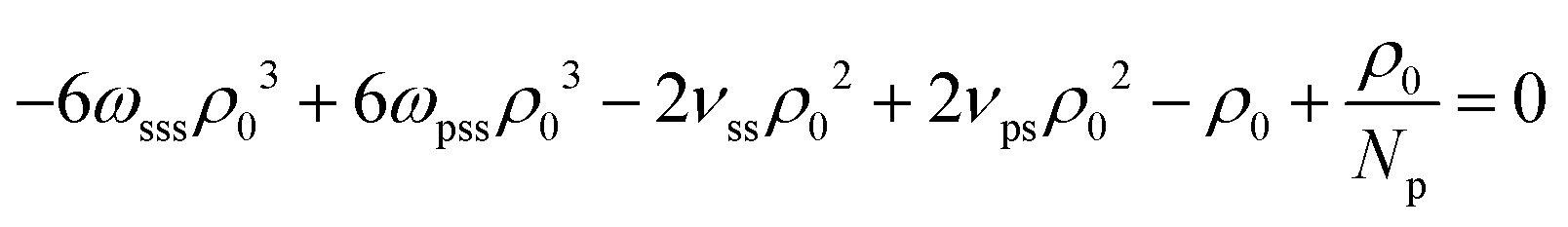 (s3). Only two of these conditions are linearly independent because s1 + s2 + s3 = C, where
  . Inspecting the expression for C we observe that this constant is actually the difference between βκT−1 for the solvent and the polymer. These are chosen to be the same in our model, therefore C = 0. Solving s1 and s2 delivers ωpps and ωpss. We clarify that cancelling the dependency of βκT−1 on xp through this approach is only approximate, because, in fact, the total density ρ0 of the mixture is affected by composition.
Acknowledgements
We are grateful to Burkhard Dünweg for a careful reading of our manuscript and numerous helpful discussions. D. M. and K. K. thank Carlos Marques for extremely fruitful collaborations over the last years. Financial support by the German Federal Ministry for Education and Research (BMBF) within the POESIE project (FKZ 13N13694) is gratefully acknowledged. Open Access funding provided by the Max Planck Society.References
- N. D. Treat, P. Westacott and N. Stingelin, Annu. Rev. Mater. Res., 2015, 45, 459–490 CrossRef CAS.
- C. Peter and K. Kremer, Faraday Discuss., 2010, 144, 9–24 RSC.
- W. Noid, J. Chem. Phys., 2013, 139, 090901 CrossRef CAS PubMed.
- G. Hernandez-Sosa, N. Bornemann, I. Ringle, M. Agari, E. Dörsam, N. Mechau and U. Lemmer, Adv. Funct. Mater., 2013, 23, 3164–3171 CrossRef CAS.
- B. Weng, R. Shepherd, K. Crowley, A. Killard and G. Wallace, Analyst, 2010, 135, 2779–2789 RSC.
- B. Derby, Annu. Rev. Mater. Res., 2010, 40, 395–414 CrossRef CAS.
- E. Maginn, AIChE J., 2009, 55, 1304–1310 CrossRef CAS.
- G. Guevara-Carrion, H. Hasse and J. Vrabec, Top. Curr. Chem., 2014, 11, 65–73 Search PubMed.
- J. Prausnitz and F. Tavares, AIChE J., 2004, 50, 739–761 CrossRef CAS.
- S. Nath, F. Escobedo and J. de Pablo, J. Chem. Phys., 1998, 108, 9905–9911 CrossRef CAS.
- S. Marrink, H. Risselada, S. Yefimov, D. Tieleman and A. de Vries, J. Phys. Chem. B, 2007, 111, 7812–7824 CrossRef CAS PubMed.
- K. Daoulas and M. Müller, Adv. Polym. Sci., 2010, 224, 197–233 CAS.
- M. Müller, J. Stat. Phys., 2011, 145, 967–1016 CrossRef.
- M. Müller and J. J. de Pablo, Annu. Rev. Mater. Res., 2013, 43, 1–34 CrossRef.
- M. Laradji, H. Guo and M. Zuckermann, Phys. Rev. E: Stat. Phys., Plasmas, Fluids, Relat. Interdiscip. Top., 1994, 49, 3199–3206 CrossRef CAS.
- I. Pagonabarraga and D. Frenkel, J. Chem. Phys., 2001, 115, 5015–5026 CrossRef CAS.
- S. Trofimov, E. Nies and M. Michels, J. Chem. Phys., 2002, 117, 9383–9394 CrossRef CAS.
- K. Daoulas and M. Müller, J. Chem. Phys., 2006, 125, 184904 CrossRef PubMed.
- D. Pike, F. Detcheverry, M. Müller and J. de Pablo, J. Chem. Phys., 2009, 131, 084903 CrossRef PubMed.
- P. Gemünden, C. Poelking, K. Kremer, D. Andrienko and K. Daoulas, Macromolecules, 2013, 46, 5762–5774 CrossRef.
- K.-X. Song, Y.-X. Jia, Z.-Y. Sun and L.-J. An, J. Chem. Phys., 2008, 129, 144901 CrossRef PubMed.
- L. Zhang, A. Sevink and F. Schmid, Macromolecules, 2011, 44, 9434–9447 CrossRef CAS.
- J. Heuser, G. Sevink and F. Schmid, Macromolecules, 2017, 50, 4474–4490 CrossRef CAS.
- F. Schmid, Handbook of Multiphase Polymer Systems, Wiley-VCG, Weinheim, 2011, vol. 1, pp. 31–80 Search PubMed.
- K. Soga, H. Guo and M. Zuckermann, Europhys. Lett., 1995, 29, 531–536 CrossRef CAS.
- K. Soga, M. Zuckermann and H. Guo, Macromolecules, 1996, 29, 1998–2005 CrossRef CAS.
- M. Müller and G. Smith, J. Polym. Sci., Part B: Polym. Phys., 2005, 43, 934–958 CrossRef.
- Y. Norizoe, K. Daoulas and M. Müller, Faraday Discuss., 2010, 144, 369–391 RSC.
- M. Hömberg and M. Müller, J. Chem. Phys., 2010, 132, 155104 CrossRef PubMed.
- A. Alexander-Katz, A. Moreira and G. Fredrickson, J. Chem. Phys., 2003, 118, 9030–9036 CrossRef CAS.
- D. Kipp and V. Ganesan, J. Phys. Chem. B, 2014, 118, 4425–4441 CrossRef CAS PubMed.
- S.-M. Hur, G. Khaira, A. Ramírez-Hernández, M. Müller, P. Nealey and J. de Pablo, ACS Macro Lett., 2015, 4, 11–15 CrossRef CAS.
- G. Sevink, M. Charlaganov and J. Fraaije, Soft Matter, 2013, 9, 2816–2831 RSC.
- P. Zhang and Q. Wang, Soft Matter, 2013, 9, 11183–11187 RSC.
- K. Binder, M. Müller, P. Virnau and L. MacDowell, Adv. Polym. Sci., 2005, 173, 1–110 CrossRef CAS.
- H. Schild, M. Muthukumar and D. Tirrell, Macromolecules, 1991, 24, 948–952 CrossRef CAS.
- F. M. Winnik, H. Ringsdorf and J. Venzmer, Macromolecules, 1990, 2415–2416 CrossRef CAS.
- H. Kojima, F. Tanaka, C. Scherzinger and W. Richtering, J. Polym. Sci., Part B: Polym. Phys., 2013, 1100–1111 CrossRef CAS.
- C. Wu and X. Wang, Phys. Rev. Lett., 1998, 80, 4092–4094 CrossRef CAS.
- J. Walter, J. Sehrt, J. Vrabec and H. J. Hasse, J. Phys. Chem. B, 2012, 116, 5251–5259 CrossRef CAS PubMed.
- D. Mukherji, M. Wagner, M. D. Watson, S. Winzen, T. E. de Oliveira, C. M. Marques and K. Kremer, Soft Matter, 2016, 12, 7995–8003 RSC.
- K. Kyriakos, M. Philipp, C. H. Lin, M. Dyakonova, N. Vishnevetskaya, I. Grillo, A. Zacconi, A. Miasnikova, A. Laschewsky, P. Müller-Buschbaum and C. M. Papadakis, Macromol. Rapid Commun., 2016, 37, 420–425 CrossRef CAS PubMed.
- Y. Yu, R. A. L. de la Cruz, B. D. Kieviet, H. Gojzewski, A. Pons, G. J. Vancso and S. de Beer, Nanoscale, 2017, 9, 1670–1675 RSC.
- S. Backes, P. Krause, W. Tabaka, M. Witt, D. Mukherji, K. Kremer and R. von Klitzing, ACS Macro Lett., 2017, 6, 1042–1046 CrossRef CAS.
- D. Mukherji and K. Kremer, Macromolecules, 2013, 46, 9158–9163 CrossRef CAS.
- C. Dalgicdir, F. Rodríguez-Ropero and N. van der Vegt, J. Phys. Chem. B, 2017, 121, 7741–7748 CrossRef CAS PubMed.
- J. J. Magda, G. H. Fredrickson, R. G. Larson and E. Helfand, Macromolecules, 1988, 21, 726–732 CrossRef CAS.
- J. Heyda, A. Muzdalo and J. Dzubiella, Macromolecules, 2013, 46, 1231–1238 CrossRef CAS.
- D. Mukherji, C. Marques and K. Kremer, Nat. Commun., 2014, 5, 4882 CrossRef PubMed.
- D. Mukherji, C. Marques, T. Stuehn and K. Kremer, J. Chem. Phys., 2015, 142, 114903 CrossRef PubMed.
- F. Tanaka, T. Koga and F. M. Winnik, Phys. Rev. Lett., 2008, 101, 028302 CrossRef PubMed.
- J. Dudowicz, K. F. Freed and J. F. Douglas, J. Chem. Phys., 2015, 143, 131101 CrossRef PubMed.
- X. Chen, W. Feng, X. Han and H. Liu, Langmuir, 2017, 33, 11446–11456 CrossRef CAS PubMed.
- T. Fukai, N. Shinyashiki, S. Yagihara, R. Kita and F. Tanaka, Langmuir, 2018, 34, 3003–3009 CrossRef CAS PubMed.
- J. Eastwood, R. Hockney and D. Lawrence, Comput. Phys. Commun., 1980, 19, 215–261 CrossRef CAS.
- G. Milano and T. Kawakatsu, J. Chem. Phys., 2009, 130, 214106 CrossRef PubMed.
- L. Livandaru, R. R. Netz and H. J. Kreuzer, Macromolecules, 2003, 36, 3732–3744 CrossRef.
- M. Müller and L. MacDowell, Macromolecules, 2000, 33, 3902–3923 CrossRef.
- I. Lifshitz, A. Grosberg and A. Khokhlov, Rev. Mod. Phys., 1978, 50, 683–713 CrossRef CAS.
- J. Zhang, D. Mukherji and K. Daoulas, Eur. Phys. J.-Spec. Top., 2016, 225, 1423–1440 CrossRef CAS.
- F. A. Detcheverry, H. Kang, K. C. Daoulas, M. Müller, P. F. Nealey and J. J. de Pablo, Macromolecules, 2008, 41, 4989–5001 CrossRef CAS.
- A. Kron, Polym. Sci. USSR, 1965, 7, 1361–1367 CrossRef.
- F. Wall and F. Mandel, J. Chem. Phys., 1975, 63, 4592–4595 CrossRef CAS.
- S. Kumar, M. Vacatello and D. Yoon, J. Chem. Phys., 1988, 89, 5206–5215 CrossRef CAS.
- V. Mavrantzas and D. Theodorou, Macromolecules, 1998, 31, 6310–6332 CrossRef CAS.
- R. Everaers, S. Sukumaran, G. Grest, C. Svaneborg, A. Sivasubramanian and K. Kremer, Science, 2004, 303, 823–826 CrossRef CAS PubMed.
- S. Edwards, Proc. Phys. Soc., 1966, 88, 265–280 CrossRef CAS.
- M. Doi and S. Edwards, The theory of polymer dynamics, Oxford University Press, New York, 1986 Search PubMed.
- D. Wu, G. Fredrickson, J. Carton, A. Ajdari and L. Leibler, J. Polym. Sci., Part B: Polym. Phys., 1995, 33, 2373–2389 CrossRef CAS.
- N. Lefévre, K. Daoulas, M. Müller, J.-F. Gohy and C.-A. Fustin, Macromolecules, 2010, 43, 7734–7743 CrossRef.
- A. Costa, M. Geoghegan, P. Vlček and R. Composto, Macromolecules, 2003, 36, 9897–9904 CrossRef CAS.
- K. Daoulas, D. Theodorou, V. Harmandaris, N. Karayiannis and V. Mavrantzas, Macromolecules, 2005, 38, 7134–7149 CrossRef CAS.
- N. Tretyakov, P. Papadopoulos, D. Vollmer, H.-J. Butt, B. Dünweg and K. Daoulas, J. Chem. Phys., 2016, 145, 134703 CrossRef PubMed.
- J. Prausnitz, R. Lichtenthaler and E. de Azevedo, Molecular Thermodynamics of Fluid-Phase equilibria, Prentice Hall PTR, USA, 1999 Search PubMed.
- G. Vogiatzis, G. Megariotis and D. Theodorou, Macromolecules, 2017, 50, 3004–3029 CrossRef CAS.
- D. Prusty, V. Pryamitsyn and M. O. de la Cruz, Macromolecules, 2018, 51, 5918–5932 CrossRef CAS.
- P. Painter, Y. Park and M. Coleman, Macromolecules, 1988, 21, 66–72 CrossRef CAS.
- E. Feng and G. Fredrickson, Macromolecules, 2006, 39, 2364–2372 CrossRef CAS.
- K. C. Daoulas, A. Cavallo, R. Shenhar and M. Müller, Soft Matter, 2009, 5, 4499–4509 RSC.
- J. Wittmer, A. Milchev and M. Cates, J. Chem. Phys., 1998, 109, 834–845 CrossRef CAS.
- G. Kamath, G. Georgiev and J. Potoff, J. Phys. Chem. B, 2005, 109, 19463–19473 CrossRef CAS PubMed.
- P. Kindt and W. Briels, J. Chem. Phys., 2007, 127, 134901 CrossRef CAS PubMed.
- P. Warren, Phys. Rev. Lett., 2001, 87, 225702 CrossRef CAS PubMed.
- M. Rubinstein and R. H. Colby, Polymer Physics, Oxford University Press, 2003 Search PubMed.
- A. Jain, B. Dünweg and R. Prakash, Phys. Rev. Lett., 2012, 109, 088302 CrossRef PubMed.
- K. Mansfield and D. Theodorou, Macromolecules, 1990, 23, 4430–4445 CrossRef CAS.
- J. Scheutjens and G. Fleer, J. Phys. Chem., 1980, 84, 178–190 CrossRef CAS.
- A. Semenov, J. Bonet-Avalos, A. Johner and J. Joanny, Macromolecules, 1996, 29, 2179–2196 CrossRef CAS.
- I. Bitsanis and G. ten Brinke, J. Chem. Phys., 1993, 99, 3100–3111 CrossRef CAS.
- C. Hoeve, E. DiMarzio and P. Peyser, J. Chem. Phys., 1965, 42, 2558–2563 CrossRef CAS.
- K. Wohl, Trans. AIChE, 1946, 42, 215–249 CAS.
| This journal is © The Royal Society of Chemistry 2018 |