DOI:
10.1039/C8SM01102H
(Paper)
Soft Matter, 2018,
14, 6043-6057
Diffusiophoretically induced interactions between chemically active and inert particles†
Received
29th May 2018
, Accepted 18th June 2018
First published on 25th June 2018
Abstract
In the presence of a chemically active particle, a nearby chemically inert particle can respond to a concentration gradient and move by diffusiophoresis. The nature of the motion is studied for two cases: first, a fixed reactive sphere and a moving inert sphere, and second, freely moving reactive and inert spheres. The continuum reaction–diffusion and Stokes equations are solved analytically for these systems and microscopic simulations of the dynamics are carried out. Although the relative velocities of the spheres are very similar in the two systems, the local and global structures of streamlines and the flow velocity fields are found to be quite different. For freely moving spheres, when the two spheres approach each other the flow generated by the inert sphere through diffusiophoresis drags the reactive sphere towards it. This leads to a self-assembled dimer motor that is able to propel itself in solution. The fluid flow field at the moment of dimer formation changes direction. The ratio of sphere sizes in the dimer influences the characteristics of the flow fields, and this feature suggests that active self-assembly of spherical colloidal particles may be manipulated by sphere-size changes in such reactive systems.
1 Introduction
Both living organisms and inanimate objects can respond to the presence of chemical gradients by moving either towards or away from high concentrations of chemical species. In the biological realm organisms are observed to orient or move in response to chemical agents. For instance, E. coli bacteria are found in glucose-rich regions indicating that they search for food and tend to migrate toward it,1,2 sperm cells are known to follow concentration gradients of chemoattractants secreted by the oocyte for fertilization,3 and there are many other examples.1,4 The ability to sense chemical gradients is not restricted to living organisms. It is well known that colloidal particles can respond to chemical gradients and move to higher or lower concentration regions through diffusiophoretic mechanisms.5–8 In this and other phoretic mechanisms, the gradient of some field across the colloidal particle gives rise to a body force, which, because of momentum conservation, induces fluid flow in the surrounding medium that causes the particle to move. The motions of motors propelled by self-phoretic mechanisms9–12 have also been observed to be affected by the presence of chemical gradients; for example, experiments have shown that bimetallic-rod and Janus motors preferentially move towards higher hydrogen peroxide concentrations.13,14 As well, simulations of sphere-dimer motors in a microfluidic channel15 and in bulk solution16 show that these motors respond to concentration gradients.
In this article, we investigate the dynamics of a pair of small colloidal particles, one of which is chemically active and converts fuel to product, while the other is nonreactive. Further, we suppose that the interactions of the fuel and product molecules with the colloidal particles are the same for the reactive particle but different for the nonreactive particle, so that the nonreactive particle can respond to the chemical gradient produced by the catalytic particle as a result of diffusiophoresis. We consider interactions such that diffusiophoresis causes motion towards high product concentrations, and situations where the reactive particle is either fixed or free to move.
These specific choices are only a few among several other possibilities. For instance, the interaction potentials may be chosen so that either or both colloidal particles may be diffusiophoretically active with different responses to gradients.17 Also, either particle may be fixed or free to move, or their internuclear separation can be fixed as in a sphere-dimer motor.18–20 All of these situations are potentially interesting to study. A study, based on a continuum description of the fluid, of the dynamics of a pair of colloidal particles each of which could be Janus particles or active or inert is related to the work presented here.21,22 In order to investigate the dynamical properties of the spheres we use deterministic continuum theory as well as coarse-grain microscopic simulations. The particle-based simulations include fluctuations relevant for experimental studies of small active colloidal particles in solution,23 and automatically account for chemical-gradient, hydrodynamic and direct intermolecular interactions between the spheres without imposing specific boundary conditions.24
The diffusiophoretic mechanism for the motion of a colloidal particle in an external concentration gradient is well known.5–8 By choosing the fixed reactive particle in our study to be diffusiophoretically inactive, it serves simply as reactive source that produces concentration gradients in the system.13–16 The nonreactive colloidal particle responds to this chemical gradient, which is analogous to an external chemical gradient, but presents some additional features as a result of pinning and reaction. We may contrast this case with that when the reactive sphere is free to move. The reactive particle again only generates concentration gradients in the system but when the two spheres closely approach we show that they form a self-assembled sphere-dimer motor that moves autonomously in solution, and we find that substantial changes in the flow fields occur at the moment of the dimer formation.
On a basic level, investigations of the mechanisms that give rise to the concentration and fluid flow fields that are responsible for the dynamics provide insight into the relative roles of chemical and hydrodynamic interactions, a topic that is important for studies of the collective dynamics of active particles.25–27 In this connection, recent experimental and computational studies have considered mixtures of chemically active and inactive spherical particles that exhibit interesting self-assembly and emergent dynamics.28–30 As in the present study, the dynamics of such mixtures will depend on both hydrodynamic and chemical, temperature, or electric fields that exist in the system.21,22,31–35
In Section 2 we present continuum solutions for the reaction–diffusion and Stokes equations for this problem, and Section 3 describes the particle-based simulation method. Sections 4 and 5 discuss the physical phenomena that are observed for fixed and freely moving catalytic spheres, respectively. The conclusions of the investigation are given in Section 6.
2 Continuum theory
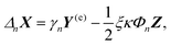
We consider two spheres, a catalytically active sphere S1 with radius R1 and a catalytically inactive sphere S2 with radius R2. These spheres, shown in Fig. 1, are taken to be separated by a distance L in three dimensional space. Two solute species A (reactant) and B (product) take part in the irreversible chemical reaction A + S1 → B + S1 on the catalytic sphere. Since we consider the case where catalytic sphere has no phoretic mobility, the interaction potentials of these species with the catalytic sphere are assumed to be the same, U1,A = U1,B, while they are different for the noncatalytic sphere, U2,A ≠ U2,B, where Ui,I is the interaction potential between the sphere i and the solute species I.
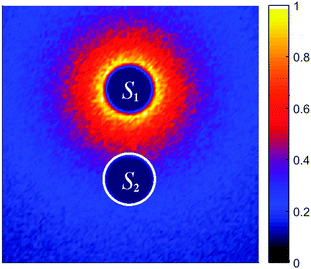 |
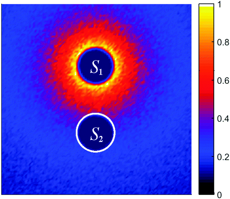
| | Fig. 1 Two spheres, one catalytically active (S1) and the other catalytically inactive (S2), are shown. The S1 sphere, as a source of concentration gradients, converts species A (reactant) to B (product) in the reaction, A + S1 → B + S1, which generates inhomogeneous concentration fields around the S2 sphere. The S2 sphere moves by the diffusiophoretic mechanisms due to the asymmetry of the concentration field in its vicinity. The numbers in the color bar indicate the normalized concentration of products (B). (The figure is constructed from simulation data described in the text. The sphere separation distance is L/σ = 3.5.) | |
In this circumstance the concentration gradient in the system arising from chemical activity on S1 will induce a body force on the noncatalytic sphere S2. The diffusiophoretic mechanism will then operate and lead to a mean velocity component along the line of centers between the two spheres due to the axial symmetry of the system. In the continuum description our interest is in the value of the mean velocity that results from this mechanism, as well as the forms of the concentration and fluid velocity fields that accompany it.
The two-sphere system can be solved in a bispherical coordinate system.20,36–39 The bispherical coordinates are (θ, η, ϕ), where 0 ≤ θ ≤ π, −∞ ≤ η ≤ ∞, and 0 ≤ ϕ ≤ 2π as shown in Fig. 2. In Cartesian coordinates (x, y, z), the relations, x = ξ![[thin space (1/6-em)]](https://www.rsc.org/images/entities/char_2009.gif) sinθcosϕ/(coshη − cosθ), y = ξsinθsinϕ/(coshη − cosθ) and z = ξsinhη/(coshη − cosθ) are satisfied with a scale factor ξ (>0).40 The surfaces of the S1 and S2 spheres are represented by the parameters η = η1(>0) and η = η2(<0), respectively. Inversely, from the values of the radii of the S1 and S2 spheres, R1 and R2, and any separation distance, L, which is greater than the sum of their radii, the bispherical coordinate parameters, ξ, η1 and η2 are found by
sinθcosϕ/(coshη − cosθ), y = ξsinθsinϕ/(coshη − cosθ) and z = ξsinhη/(coshη − cosθ) are satisfied with a scale factor ξ (>0).40 The surfaces of the S1 and S2 spheres are represented by the parameters η = η1(>0) and η = η2(<0), respectively. Inversely, from the values of the radii of the S1 and S2 spheres, R1 and R2, and any separation distance, L, which is greater than the sum of their radii, the bispherical coordinate parameters, ξ, η1 and η2 are found by  ,
,  , and
, and  .
.
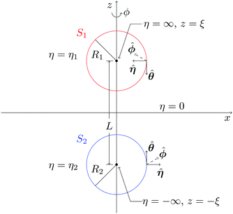 |
| | Fig. 2 Bispherical (θ, η, ϕ) and Cartesian (x, y, z) coordinates for two spheres. The catalytic sphere S1 (red) with radius R1 and noncatalytic sphere S2 (blue) with radius R2, separated by a distance L, can be specified by variables η = η1 and η = η2, respectively. The system is axisymmetric in the angle ϕ about the z axis that lies along the line connecting the centers of the two spheres. The hat notation is used to indicate unit vectors. | |
2.1 Concentration field
We assume the Péclet number is small so that fluid advection may be neglected and the steady-state concentration field of species A, cA, can be found from the solution of the diffusion equation,subject to the radiation and reflecting boundary conditions,
(J·![[small eta, Greek, circumflex]](https://www.rsc.org/images/entities/b_i_char_e108.gif) )η=η1 = )η=η1 = ![[k with combining macron]](https://www.rsc.org/images/entities/i_char_006b_0304.gif) 0cA(η = η1), 0cA(η = η1), |
| | | (J·)η=η2 = 0, | (2) |
on the S1 and S2 spheres, respectively. Here J = −D∇cA is the diffusion flux of species A, D is the common diffusion constant of A and B, and 0 = k0/(4πR12), where k0 is the intrinsic reaction rate coefficient. There are only A particles infinitely far from the spheres so that cA(r → ∞) = c0.
The total concentration c0 = cA + cB is conserved in the reaction–diffusion system with the boundary conditions on the surfaces of the spheres and infinity, and we can write cA = c0 − cB locally; thus, we can eliminate cA and consider only cB. In bispherical coordinates, the concentration of B is now given by
| | 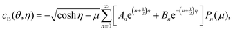 | (3) |
where
Pn(
μ) is a Legendre function and
μ = cos
θ. The
An and
Bn coefficients may obtained by following the same procedure used to obtain the solution for sphere dimers.
20
2.2 Particle velocity, streamlines and flow field
We examine two situations, the first where the catalytic sphere is fixed in space by an external force and the second where it free to move and the system is force-free. Different velocity fields arise in these cases and give rise to dynamics corresponding to physically different phenomena.
2.2.1 Fixed catalytic sphere.
We suppose that the catalytic sphere S1 is fixed in space by external force and the noncatalytic sphere S2 is able to move in the solution. The concentration field around the S1 is asymmetric as given by eqn (3); hence, a flow is generated at the surface of the S2 sphere by the diffusiophoretic mechanism.7,8 The slip velocity is the fluid velocity at the outer edge of a boundary layer beyond which the interaction potentials vanish, and is given in the body-fixed frame of the sphere by| | vs = −κ(I − ![[n with combining circumflex]](https://www.rsc.org/images/entities/b_i_char_006e_0302.gif) )·∇cB, )·∇cB, | (4) |
where I is the unit dyadic, the surface normal vector,| |  | (5) |
is the diffusiophoretic factor, with ![[small mu, Greek, macron]](https://www.rsc.org/images/entities/i_char_e0cd.gif) the shear viscosity, kB the Boltzmann constant, and T the temperature.8,12
the shear viscosity, kB the Boltzmann constant, and T the temperature.8,12
The Reynolds number is assumed to be small so that viscous forces dominate inertial forces and the fluid flow field outside of the boundary layer is found by solving the Stokes equation with the incompressibility condition,
| | | ∇p = ∇2v, ∇·v = 0, | (6) |
subject to the boundary conditions in the laboratory frame of reference,
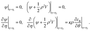
| | | vη=η1 = 0, vη=η2 = (V + vs)η=η2, | (7) |
where
p is the pressure,
v the fluid velocity field, and
V the velocity of the noncatalytic sphere.
Introducing the stream function ψ, which is related to the flow velocity by v = ![[small phi, Greek, circumflex]](https://www.rsc.org/images/entities/b_i_char_e0b5.gif) /ρ × ∇ψ, where ρ = ξsinθ/(coshη − μ), one may replace the Stokes equation with the incompressibility condition in terms of stream functions by36,40
/ρ × ∇ψ, where ρ = ξsinθ/(coshη − μ), one may replace the Stokes equation with the incompressibility condition in terms of stream functions by36,40
where
E4 =
E2(
E2) and
E2 = (cosh
η −
μ)/
ξ2[∂/∂
η{(cosh
η −
μ)∂/∂
η} + (1 −
μ2)∂/∂
μ{(cosh
η −
μ)∂/∂
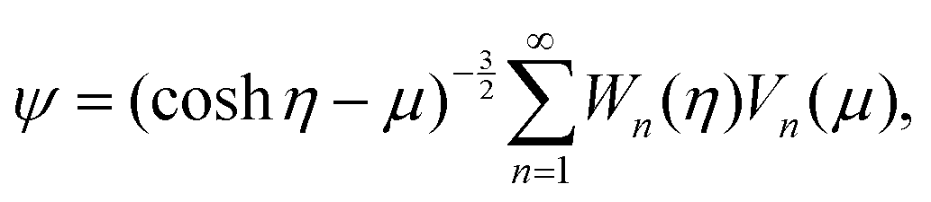
μ}]. This equation has an exact solution given by
36| |  | (9) |
where
Wn(
η) =
ancosh(
n − ½)
η +
bnsinh(
n − ½)
η +
cncosh(
n +
![[/]](https://www.rsc.org/images/entities/char_e0ee.gif)
)
η +
dnsinh(
n +
)
η and
Vn(
μ) =
Pn−1(
μ) −
Pn+1(
μ). The unknown coefficients
an,
bn,
cn, and
dn in
eqn (9) are determined by boundary conditions at the outer edges of the boundary layers around the S
1 and S
2 spheres,
i.e.eqn (7). In the laboratory frame where the motor moves with velocity
V, these boundary conditions are given in terms of the stream function by
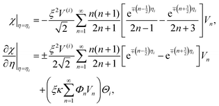
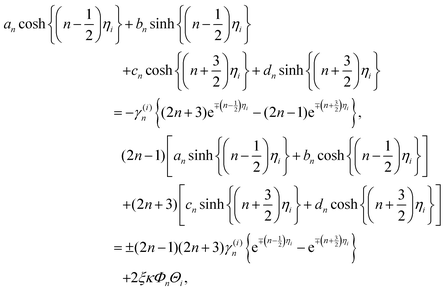
| |  | (10) |
By writing

in
eqn (9), we can replace the boundary conditions,
eqn (10) in terms of
χ by
| |  | (11) |
Here,

can be expressed in a series of Legendre function
Pn, (1 −
μ2)
Pn and
μVn are rewritten by Gegenbauer functions
Vn−1 and
Vn+1, and (1 −
μ2)d
Pn/d
μ is rewritten by
Vn.
20,36,41 Then, we may expand the right sides of
eqn (11) for
η =
η2 in a series of
Vn as
| |  | (12) |
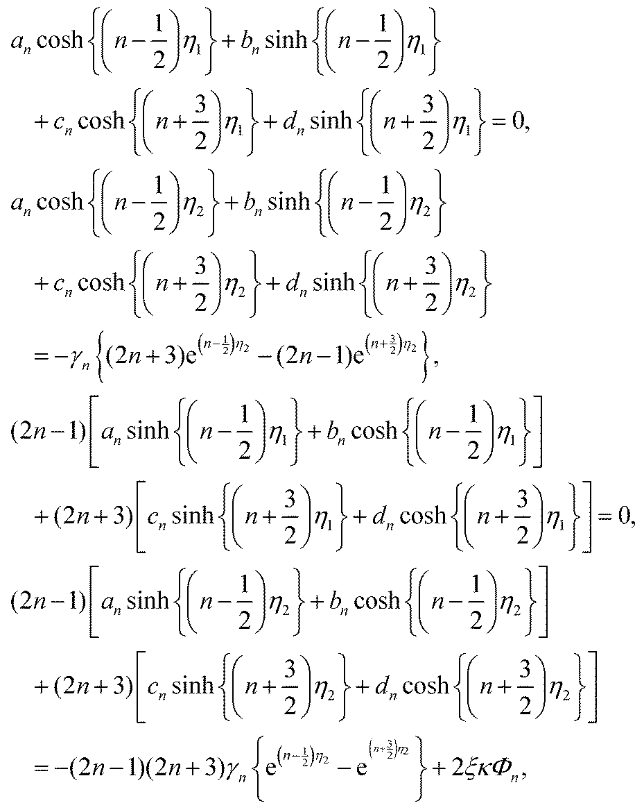
Since both sides of eqn (12) are expanded in a series of Gegenbauer function Vn, we can determine the unknown coefficients of Wn(η) in eqn (9) from the following equations:
| | 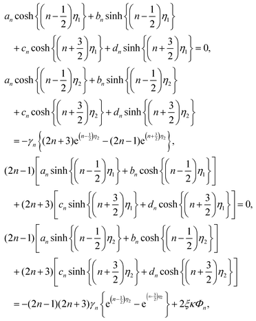 | (13) |
where
γn =
fnV and
fn is given in
Table 1 in the Appendix. The solution of the above equations for the unknown coefficients
an,
bn,
cn,
dn is expressed by
| |  | (14) |
where
X = {
an,
bn,
cn,
dn},
Y(e) = {
Y(2)n,
Y(4)n,
Y(6)n,
Y(8)n}, and
Z = {
z(1)n,
z(2)n,
z(3)n,
z(4)n}. The elements of the vectors are given in
Table 1 in the Appendix. The solution for two inactive spheres can be obtained easily by taking
κ = 0, which gives
X =
γnY(e)/
Δn. In this case, one colloidal sphere (S
2) with constant velocity
V moves to the other sphere (S
1) fixed in space.
The forces (F1,F2) on the individual spheres (S1,S2) are given by integrating the stress on the surface of the boundary layer,  (i = 1, 2), where Πi,z = ẑ·Πi and Π is the stress tensor. The system is symmetric around the azimuthal angle ϕ and only the force in the z-direction needs to be considered. The analytic expressions for the force exerted on the spheres by the fluid are given in Stimson and Jeffery36 as
| | 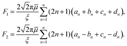 | (15) |
The velocity can be found from these force expressions. Since no external force is applied to the S2 sphere, although the S1 sphere is fixed in space by an external force, the total force on the S2 sphere at the outer edge of the boundary layer is zero, F2 = 0. Noting that γn = fnV, one can find the following expression for velocity of the noncatalytic sphere,
| | 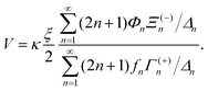 | (16) |
Also, the force
F1 exerted on the fixed catalytic sphere by the fluid found here is used for the plots in
Fig. 10.
2.2.2 Freely moving catalytic sphere.
We now suppose that both spheres are free to move and construct the solutions for this force-free case. Letting the velocities of the S1 and S2 spheres be V(1) and V(2), respectively, one may replace the boundary conditions in eqn (7) by| | | vη=η1 = (V(1))η=η1, vη=η2 = (V(2) + vs)η=η2. | (17) |
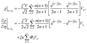
Then the boundary conditions for the stream function are| | 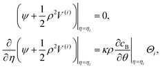 | (18) |
where Θ1 = 0, Θ2 = 1, and i = 1, 2.
In this case, the boundary conditions for streamlines in eqn (18) are rewritten in terms of  by
by
| |  | (19) |
As discussed previously, we may expand the right sides of eqn (19) in a series of Gegenbauer function Vn as
| |  | (20) |
where the upper and lower signs are taken for
i = 1 and 2, respectively.
Since both sides of eqn (20) are expanded in a series of Vn, we can determine the unknown coefficients of Wn(η) in eqn (9) from the following equations:
| |  | (21) |
where
γ(i)n =
fnV(i) and the upper and lower signs correspond to
i = 1 and 2, respectively.
The solution of the above equations for the unknown coefficients an, bn, cn, dn is given by
| |  | (22) |
where
X = {
an,
bn,
cn,
dn},
Y(o) = {
Y(1)n,
Y(3)n,
Y(5)n,
Y(7)n},
Y(e) = {
Y(2)n,
Y(4)n,
Y(6)n,
Y(8)n}, and
Z = {
z(1)n,
z(2)n,
z(3)n,
z(4)n}. The elements of the vectors are given in
Table 1 in the Appendix. Applying the force-free conditions on both the spheres,
F1 =
F2 = 0 in
eqn 15, one can find the solution for the velocities of the S
1 and S
2 spheres as
| |  | (23) |
where
| |  | (24) |
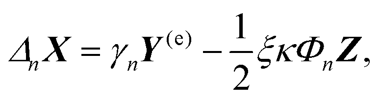
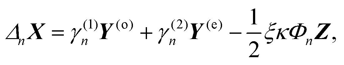
The solutions for two inactive spheres moving with constant velocities V(1) and V(2) along the axisymmetric direction can be obtained easily by setting κ = 0, which gives X = (γ(1)nY(o) + γ(2)nY(e))/Δn. Also, the solutions for the sphere-dimer can be obtained by setting V(1) = V(2) = V, which gives ΔnX = γnY − ½ξκΦnZ, where Y = Y(o) + Y(e) and γn = γ(1)n = γ(2)n. This expression is consistent with the formula given earlier.20,42
3 Microscopic dynamics
The analytical results for continuum theory are exact given the formulation of the problem on which they are based. In particular, they rest on the deterministic continuum description of the fluid and solute concentration as described by the Stokes and diffusion equations, supplemented with boundary conditions on the fluid velocity and concentration fields. The former boundary condition accounts for the fluid dynamics and the latter boundary condition describes chemical reactions on the sphere. The fluid viscosity, diffusion constant and reaction rates of chemical species are specified as input parameters to solve the equations. The Reynolds and Péclet numbers are assumed to be small.8,9,20,37,38 This is an appropriate description for a large macroscopic particle. However, in many experiments, the active particles have micrometer or nanometer dimensions and for such systems thermal fluctuations should be taken into account.23,25–27,29,30 In addition, as one moves to small nanometer23 or even Angstrom12 scales the assumptions of continuum dynamics may no longer apply.
The coarse-grain particle-based simulations do not make such assumptions. The input parameters are the intermolecular potentials and multiparticle collision parameters for the solvent.24 The resulting dynamics then yields all other properties such as the transport coefficients of the system, and other dimensionless numbers that characterize the system. One can show that on long distance and times scales the continuum hydrodynamic and diffusion equations are recovered,43 but the dynamics is not restricted to this limit. Consequently, it is of interest to examine the extent to which the continuum model can capture the active dynamics of these small particles.20,44
The coarse-grain microscopic dynamics we employ combines molecular dynamics (MD) with multiparticle collision (MPC) dynamics.43,45 More specifically, the fluid is composed of Ns point particles of mass m with positions ri and velocities vi, where i = 1,…,Ns. There are no explicit intermolecular potentials among these fluid particles and their interactions are accounted for by multiparticle collisions. The dynamics consists of two alternating steps: streaming and collision. In the streaming steps of duration h, all particles in the system move by Newton's equations of motion with forces determined by the sphere–sphere and sphere–solvent intermolecular potentials. At each collision time the solvent particles are sorted into cubic cells of side length a, which is larger than the mean free path, and their relative velocities are rotated around a randomly oriented axis by a fixed angle α with respect to the center-of-mass velocities of each cell. The velocity of particle i after collision is given by vi(t + h) = vcm(t) + ![[scr R, script letter R]](https://www.rsc.org/images/entities/char_e531.gif) (α)(vi(t) − vcm(t)), where (α) is the rotation matrix,
(α)(vi(t) − vcm(t)), where (α) is the rotation matrix,  is the center-of-mass velocity of the particles in the cell to which the particle i belongs, and Nc is the number of particles in that cell. A random shift of the collision lattice is applied at every collision step to ensure Galilean invariance.46 The dynamics locally conserves mass, momentum and energy.24
The spheres interact with the fluid particles through repulsive Lennard-Jones (LJ) potentials, U = 4ε[(σ/r)12 − (σ/r)6] + ε for r < 21/6σ and U = 0 for r ≥ 21/6σ with energy ε and distance σ parameters. In addition, repulsive LJ potentials are employed to take into account excluded volume interactions between the two spheres with σs denoting the value of σ in this case. In order to make only the noncatalytic sphere hydrodynamically active, we choose the interaction energies of the A and B molecules with the S1 catalytic sphere to be the same (εA = εB = ε) and those with the S2 noncatalytic sphere to be different (εB < εA = ε). Setting εB < εA, so that the A particles are more strongly repelled from the S2 sphere than the B particles, causes it to move towards the S1 sphere; hence B plays the role of chemoattractant. An irreversible chemical reaction A → B takes place on the S1 sphere with intrinsic reaction rate k0 whenever A encounters S1. Collisions of A or B particles with the S2 sphere do not lead to reaction. To maintain the system in a steady state, the B particles are converted to A at a distance dp (= Lb/2) far from the spheres.
All quantities are reported in dimensionless units where length, energy, mass and time are measured in units of the MPC cell length a = σ/2, ε, the solvent mass m, and  , respectively. The cubic simulation box with linear dimension Lb = 50 and periodic boundary conditions in all dimensions is divided into Lb3 = 503 cubic cells. Multiparticle collisions are carried out in each cell by performing velocity rotations by an angle α = 120° about a randomly chosen axis every collision time h = 0.1. The average solvent number density is c0 = 10 and the temperature is kBT = 1. The MD time step is Δt = 0.01. The energy parameters for the S2 sphere-fluid repulsive LJ potentials are εA = 1.0 and εB = 0.1 for A and B, respectively, while εA = εB = 1.0 for the S1 sphere. The size parameters are σ = 2 and σs = 4 to give effective sphere radii of R1 = R2 = 21/6σ. The sphere mass is taken to be M = 4πσ3c0/3 corresponding to neutral buoyancy. The intrinsic reaction rate constant for the A + S1 → B + S1 reaction can be estimated from simple collision theory so that
  . The transport properties of the fluid depend on h, α, and Nc. The fluid viscosity is = mNcν = 7.9, where ν is the kinematic viscosity, and the common A and B diffusion constant is D = 0.0611. The Schmidt number is Sc = ν/D = 13 > 1, which ensures that momentum transport dominates over mass transport, the Reynolds number Re = c0Va/ < 0.1, implying that viscosity is dominant over inertia, and the Péclet number Pe = Va/D < 1, diffusion being dominant over fluid advection.
The parameter values given above are used as input to obtain the analytic solutions in the continuum theory. For example, the factor κ in eqn (5) is obtained from the repulsive cut-off LJ potentials with the energy parameters εA and εB given in simulations, along with the viscosity from the microscopic model. Using the analytical continuum solutions and simulations of the microscopic equations of motion, we can discuss the physics underlying dynamics of these two-sphere systems. Since the phenomena depend on whether the catalytic sphere is fixed or free to move, we discuss these two cases separately.
4 Dynamics with a fixed catalytic sphere
The process by which a noncatalytic sphere responds to the chemical gradient produced by a fixed catalytic sphere and is captured by it has been studied earlier.47,48 Here we reexamine this process by making use of analytical solutions and extensive simulations of the microscopic model. The dynamical processes that enter this seemingly simple process involve effects that govern the velocity of the noncatalytic sphere and lead to its eventual capture. At large radial distances between the spheres the concentration of product B in the vicinity of S2 is low and so is its velocity. As the distance decreases the concentration of B increases leading to an increased velocity but as the spheres approach closely more complex interactions lead to the capture event. We are able to probe the details of the mechanism responsible for the capture process through an analysis of the concentration and fluid flow fields that accompany the dynamics.
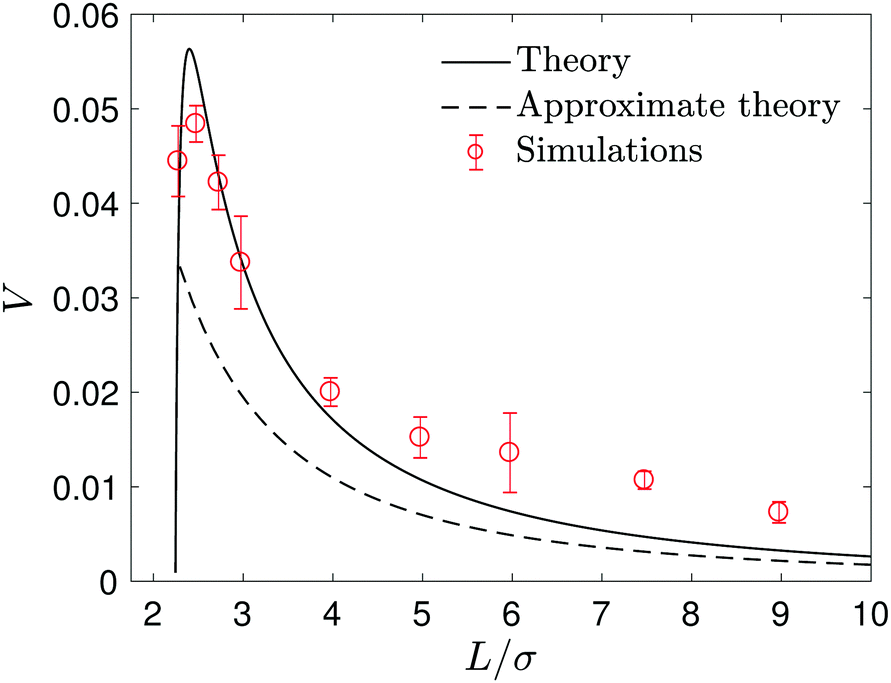
The velocity of the S2 sphere, V, is plotted in Fig. 3 as a function of the distance L separating the centers of the two spheres. The figure shows the expected increase in velocity as the S2 sphere approaches the S1 sphere until, at a short distance, it begins to decrease as the capture event takes place. The figure compares the simulation results with the exact analytical continuum theory result in eqn (16). The results are also compared with an approximate theory where the two spheres are assumed to be separated by a large distance. In this case, the concentration field may be approximated by calculating it in the absence of the S2 sphere47,48 as follows. Taking the origin of a spherical polar coordinate (r1,θ1,ϕ1) at the center of the S1 sphere in Fig. 2, the B species concentration field may be obtained from the solution of the diffusion eqn (1) subject to the radiation boundary condition in eqn (2) as
| |  | (25) |
where
kD = 4π
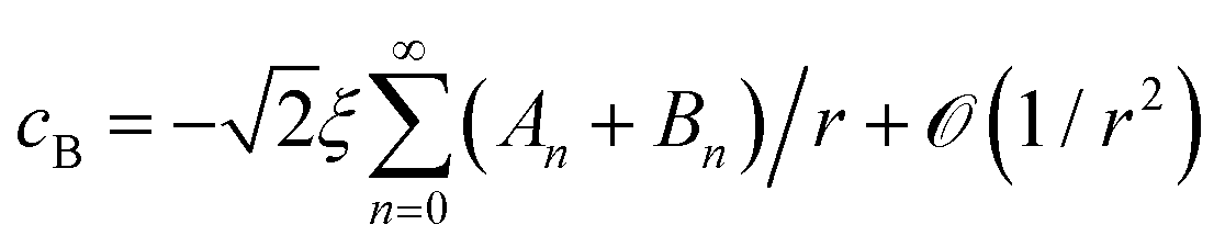
R1D is the Smoluchowski rate coefficient. This far-field concentration field can be also obtained from the approximation of the exact solution of the two spheres in large distance,
,
20 where a new spherical polar coordinate (
r,
ϑ,
ϕ) in
Fig. 2 is chosen sharing the origin, by taking the limit of
η2 → −∞ (
R2 → 0) and
L → ∞ and noting that the
n = 0 term is sufficient.
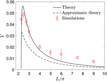 |
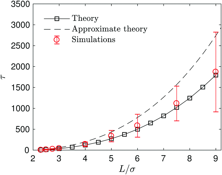
| | Fig. 3 The velocity V of the noncatalytic S2 sphere as a function of the separation L between the S2 and S1 catalytic spheres. The black solid line is the exact solution calculated from continuum hydrodynamic theory in eqn (16) and the black dashed line is the approximate velocity Va from eqn (27) that is valid for large L. The red circles with error bars are the results of microscopic simulations. Averages were obtained from 80 realizations of the dynamics. | |
The approximation to the propulsion velocity of the S2 sphere may be then found by averaging the slip velocity like eqn (4) at the edge of the boundary layer of the S2 sphere8,12,49 in a coordinate system (r2, θ2, ϕ2) where the origin is at the center of the S2 sphere. The result is
| | 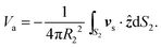 | (26) |
Here,
ẑ is a unit vector along the line of centers of the two spheres and defines the
z-axis of the spherical polar coordinate system. Using the relation
r12 =
r22 +
L2 − 2
r2Lcos
θ2, one obtains
cB(
r2) from
eqn (25) and hence an approximate expression for the sphere velocity for distances
L ≫
R2 given by
| | 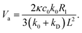 | (27) |
As expected, the approximate and exact theories agree for large sphere separations where both have a
L−2 power law behavior, but significant deviations are seen a short distances. The discrepancies between the microscopic simulations and exact continuum theory may be due to the use of soft potential functions and features of microscopic dynamics taking place in the boundary layer which are not captured by the simple boundary conditions in the continuum model, which likely manifest themselves more strongly at large separations where the product concentrations and gradients are small.
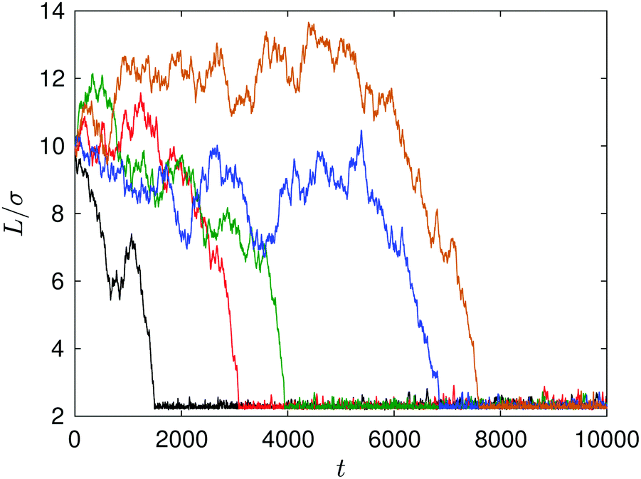
In the microscopic simulations the colloidal particles undergo Brownian motion as a result of thermal fluctuations, as well as directed motion due to diffusiophoresis. Fig. 4 shows some examples of noncatalytic sphere trajectories. At large distances (L/σ > 8) the noncatalytic sphere exhibits small thermal fluctuations in its displacement which are less than its radius, as well as larger random displacements. When L/σ < 6, diffusiophoretic interactions are stronger and the deterministic component of the motion dominates. Thus, fluctuations lead to a dispersion of capture times seen in Fig. 4, and only the average in Fig. 5 can be compared to the deterministic theory.
 |
| | Fig. 4 Plot of the distance between the fixed catalytic and moving noncatalytic spheres as a function of time. Five realizations of the dynamics are shown, each with an initial separation L/σ = 10. Contact occurs at approximately L/σ ∼ 2.3. The time where the distance achieves its minimum value is the capture time (see Fig. 5). | |
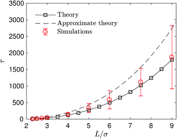 |
| | Fig. 5 Capture time τ as a function of the initial separation L between the spheres. The black solid line with squares is the exact continuum solution and the dashed line is the approximate result. The red circles denote the simulation results obtained from averages over 80 realizations. | |
The capture time, τ, which is defined by the time it takes the S2 sphere, initially at L, to reach the S1 sphere, i.e., the spheres are separated by a distance equal to the sum of their radii, R1 + R2. The time τ can be calculated easily by integrating the velocity (eqn (27)) to obtain the simple expression, τ = (k0 + kD)(L3 − (R1 + R2)3)/(2κc0k0R1). Fig. 5 shows how τ varies with L. The exact continuum solutions agree well with simulations, while here are discrepancies with the approximate theory.
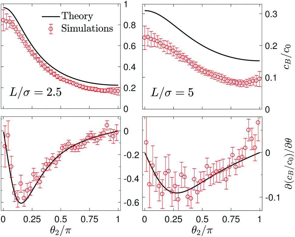
The concentration and fluid velocity fields vary during the capture process, and these variations play a role in determining the details of the capture mechanism. The B species concentration fields and their gradients on the surface of the S2 sphere are shown in Fig. 6. The concentration field decays as 1/r at long distances20 but again there are discrepancies in the magnitude of the field close to the S2 sphere. Such discrepancies might be expected because the dynamics in the finite-size boundary layer cannot be simply represented by the continuum boundary conditions. It is interesting that the tangential gradient of this field on the surface corresponds very closely to that of the continuum model. Consequently, even though the microscopic nature of the concentration fields is manifest in the boundary layer, the gradient, which determines the propulsion, is accurately given by the continuum theory. As a result many of the other observable properties are accurately given.
 |
| | Fig. 6 Normalized concentration fields cB/c0 and the tangential gradients ∂(cB/c0)/∂θ2 on the surface of the noncatalytic S2 sphere (R2/σ = 21/6) for L/σ = 2.5 (left column) and L/σ = 5 (right column), respectively. The angle θ2 is the polar angle in spherical polar coordinates where the origin is at the center of the S2 sphere. | |
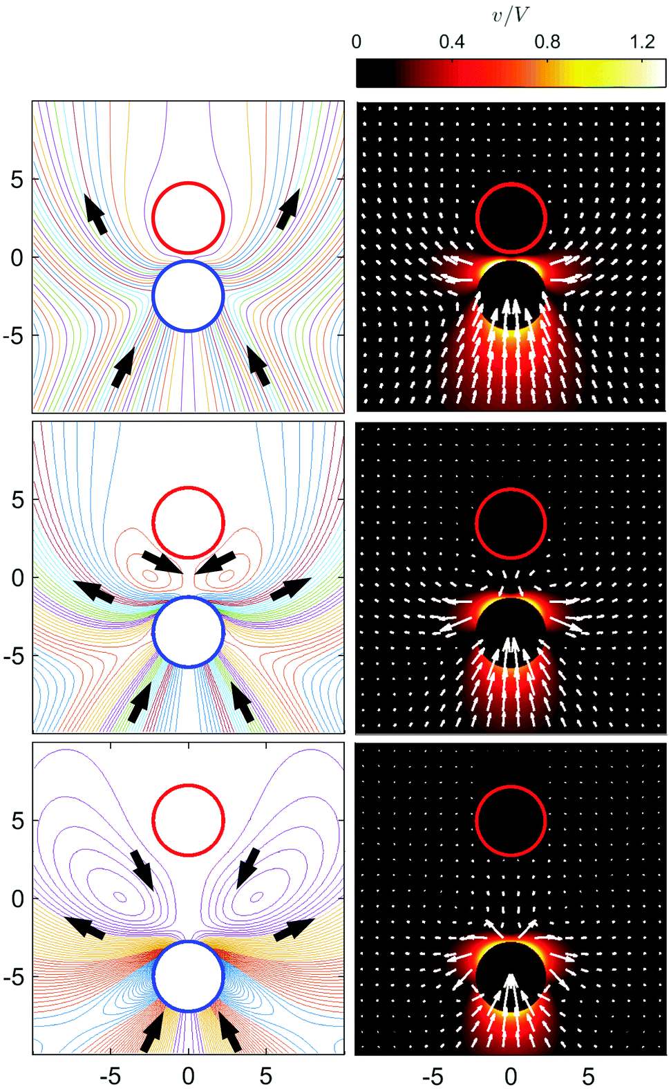
The velocity fields generated by the moving S2 sphere present a more interesting and complex structure as a function of L. Fig. 7 shows the streamlines and flow fields in the laboratory frame of reference. The streamlines are plotted by setting ψ equal to a constant. At large separations, we see that the fluid near the head of the S2 sphere (portion closest to the S1 sphere) is pushed to the lateral directions (in the xy plane) with respect to the axisymmetric z axis, and executes broad fluid circulation near the S1 sphere. Fluid also flows towards the rear of the S2 sphere. The flow near the S2 sphere shows a puller-like behavior; i.e., fluid enters from the front and back and is expelled from the sides.32,50 (A pusher-like behavior can be also seen in our system if εB > εA.) As the two spheres approach each other (L/σ ∼ 3.5) the circulating flows between and to the sides of the spheres reduce in size and disappear, leaving a puller-like flow pattern. Near the contact distance (L/σ ∼ 2.5), the fluid is pushed from the back to the front of two spheres.
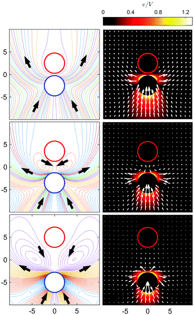 |
| | Fig. 7 Streamlines and flow fields in the laboratory frame of reference. In the left column, streamlines are shown near the two spheres with flow directions indicated (black arrows) and, in the right column, the flow fields (white arrows) and their magnitudes (color maps),  , are presented. The first, second, third rows are for L/σ = 2.5, 3.5, 5. In the color maps, the magnitude of the fluid velocity v is scaled by the sphere velocity V, where V = 0.053, 0.023, 0.011 for L/σ = 2.5, 3.5,5, respectively. The red and blue circles indicate the S1 catalytic and S2 noncatalytic spheres. , are presented. The first, second, third rows are for L/σ = 2.5, 3.5, 5. In the color maps, the magnitude of the fluid velocity v is scaled by the sphere velocity V, where V = 0.053, 0.023, 0.011 for L/σ = 2.5, 3.5,5, respectively. The red and blue circles indicate the S1 catalytic and S2 noncatalytic spheres. | |
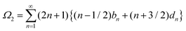
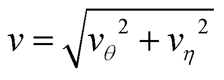
That the flow patterns are affected by the pinning of the catalytic sphere are clearly seen in the plots of the far field streamlines in Fig. 8. The flow near the spheres resembles that due to stresslet fields (similar to that for L/σ ∼ 3.5 and ∼5 in Fig. 7), but at distances far from the spheres (see Fig. 8(b) and (c)) the flow resembles a drift flow (Stokeslet).51 When the separation between the spheres is large (Fig. 8(d), L/σ ∼ 7.5), the flow circulation (stresslet fields) expands to occupy a larger portion of space, but a drift flow (Stokeslet) again appears when viewed at large distances from the spheres. These far-field flows are characterized quantitatively by calculating the magnitude of fluid velocity  , where v = vθ
![[small straight theta, Greek, circumflex]](https://www.rsc.org/images/entities/b_i_char_e12d.gif) + vη,40 as shown in Fig. 9. For example, at L/σ = 7.5, one sees a 1/r2 decay, characteristic of stresslets, for distances up to approximately r/σ ∼ 20, but eventually the flow velocity decays asymptotically as 1/r. As the separation distance decreases, it is notable that the flow velocity increases, the stresslet contribution disappears, and the Stokeslet contribution increases. The asymptotic expressions are found by introducing the spherical polar coordinates (r, ϑ, ϕ) in Fig. 2, where two coordinate systems share the origin, and expanding the variables θ and η in terms of 1/r. Then one may obtain asymptotic expressions for flow velocity up to
+ vη,40 as shown in Fig. 9. For example, at L/σ = 7.5, one sees a 1/r2 decay, characteristic of stresslets, for distances up to approximately r/σ ∼ 20, but eventually the flow velocity decays asymptotically as 1/r. As the separation distance decreases, it is notable that the flow velocity increases, the stresslet contribution disappears, and the Stokeslet contribution increases. The asymptotic expressions are found by introducing the spherical polar coordinates (r, ϑ, ϕ) in Fig. 2, where two coordinate systems share the origin, and expanding the variables θ and η in terms of 1/r. Then one may obtain asymptotic expressions for flow velocity up to ![[scr O, script letter O]](https://www.rsc.org/images/entities/char_e52e.gif) (1/r2) as
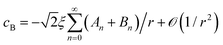
(1/r2) as
| |  | (28) |
where
and
. The details are given in the Appendix.
 |
| | Fig. 8 Far-field streamlines for various sphere separations, (a) L/σ = 2.5 (b) L/σ = 3.5 (c) L/σ = 5 (d) L/σ = 7.5. | |
 |
| | Fig. 9 The magnitude of fluid velocity,  , for ϑ = π/2 as a function of distance r, where the spherical polar coordinates (r, ϑ, ϕ) are taken with a common origin in Fig. 2. The black, red, green, blue, brown, magenta lines (from top to bottom) correspond to the separation distances, L/σ = 2.5, 3.5, 5, 7.5, 10, 15, respectively. , for ϑ = π/2 as a function of distance r, where the spherical polar coordinates (r, ϑ, ϕ) are taken with a common origin in Fig. 2. The black, red, green, blue, brown, magenta lines (from top to bottom) correspond to the separation distances, L/σ = 2.5, 3.5, 5, 7.5, 10, 15, respectively. | |
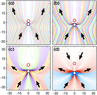
Since the fluid between the spheres flows from the S1 to S2 spheres with a broad circulation pattern, one may expect that the force the fluid exerts on the fixed catalytic sphere is in the same direction; i.e., an attractive force. (If εB > εA then the flow directions are reversed and one has a repulsive force.) The force is given by eqn (15) and is plotted in Fig. 10, along with the simulation result. In the microscopic simulations, the force is calculated by summing the forces on the catalytic sphere due to all of the fluid particles. The continuum theory and simulations agree very well. The force is almost zero for large L, and becomes more negative (attractive) as L decreases, reaching its largest negative value at L/σ ∼ 2.5, near the contact distance, L/σ ∼ 2.25. If L decreases further, the force take positive (repulsive) values.
 |
| | Fig. 10 The force on the catalytic sphere exerted by fluid. The black solid line and red circles correspond to the continuum theory and simulations, respectively. Negative values (−z direction in Fig. 2) imply the force is attractive. | |
5 Dynamics with a moving catalytic sphere
We now consider the situation where both spheres are free to move. The concentration fields produced by the catalytic sphere are unchanged from the fixed-sphere case. Using the continuum theory, the velocities of both spheres can be computed from eqn (23) and they are plotted in Fig. 11, along with the simulation results. The continuum theory and microscopic simulation results are in good agreement. Now the S1 and S2 spheres move towards each other, but with different velocities as shown in the figure. The velocity of the S2 sphere is much larger than that of the S1 sphere, and the velocity difference V(2) − V(1) is shown in the inset of the figure. For comparison, this difference is compared with that for a fixed S1 sphere, V = V(1) = 0, (dashed line in the inset). Although the S2 sphere moves by the diffusiophoretic mechanism, the motion of the S1 sphere is induced by the fluid flow generated by the S2 sphere.
 |
| | Fig. 11 Plot of the velocities V(1) and V(2) of the S1 and S2 spheres in a force-free system. The solid blue and red lines denote the continuum theoretical values of V(1) and V(2), respectively, while the circles with error bars are the microscopic simulation results. The inset shows the velocity difference V(2) − V(1) (solid lines) and, for comparison, the velocity of the S2 sphere (dashed line) when the S1 sphere is fixed in space (eqn (16)). | |
Note that although the velocities of the two spheres have opposite signs (− for S1 and + for S2) as they approach, the sign of the S1 velocity changes so that both sphere velocities are positive (+z) as the two spheres meet to form a self-propelled sphere-dimer that moves with the S1 sphere at its head (see Movie 2, ESI†).19,20 In contrast to the sphere-dimer motors previously studied that are made from spheres with a rigid bond, this sphere-dimer motor self-assembles from isolated spheres to form a bound pair with a bond length that may fluctuate around a mean value depending on parameters used. Once the sphere dimer is formed by self-assembly it behaves like the sphere-dimer with a fixed bond length. Similar motion of two spheres was observed in a numerical study of a thermocapillary system consisting of a solid particle and a gas bubble.52
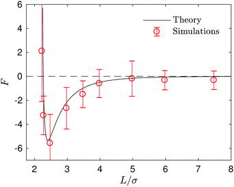
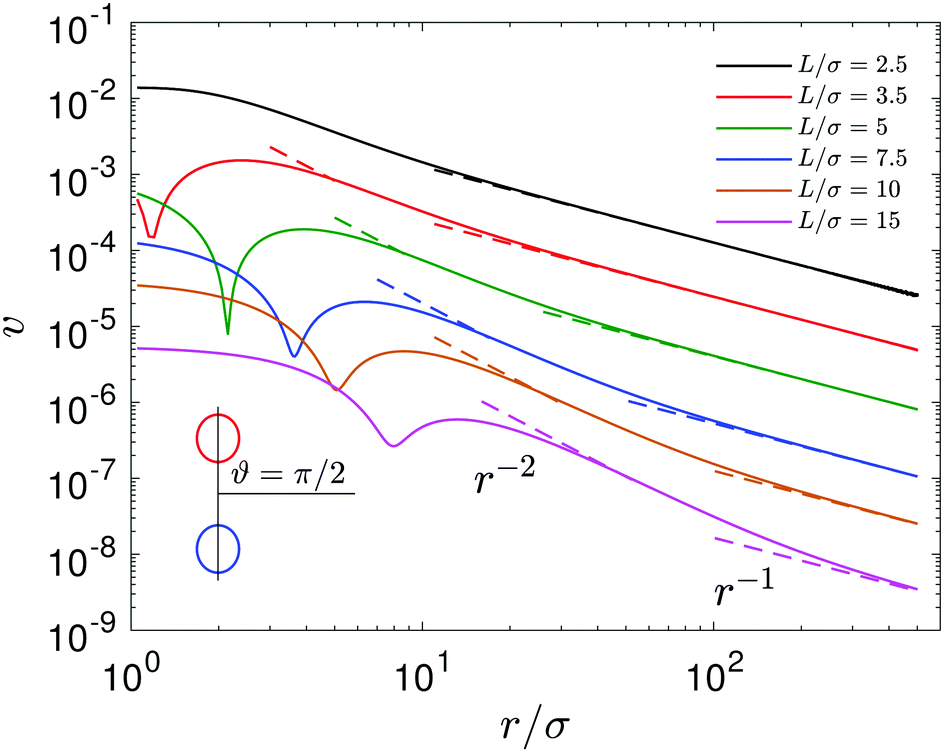
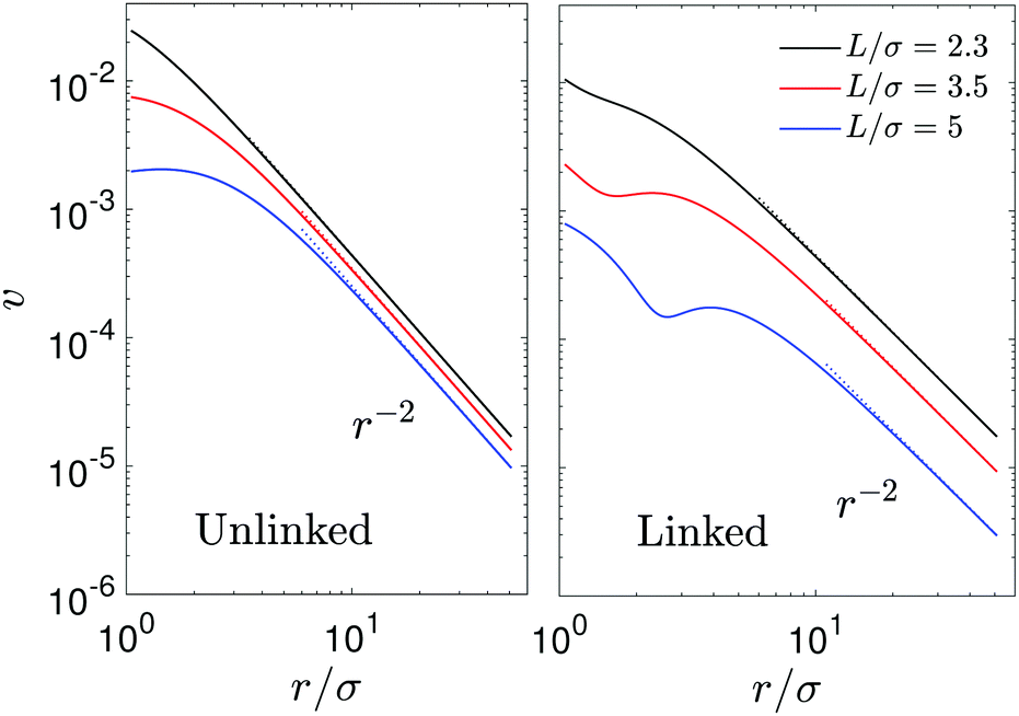
The streamlines and flow field are shown in Fig. 12 (left two columns) in the laboratory frame of reference. When L is relatively large (L/σ = 5), the streamlines are roughly similar to those when the S1 sphere is fixed but there is no local fluid circulations at small distances from the spheres and no drift flow at large distances. The fluid flow near the S2 sphere exhibits a puller-like pattern and near the S1 sphere fluid is simply dragged to the S2 sphere. As discussed above, this difference is attributed to the contributions of Stokeslets in a forced system and these effects are pronounced at small L (L/σ = 2.3, 3.5). The streamlines in a force-free system do not significantly change at small separations, while those in a forced system are more distorted in the direction of the applied external force (Fig. 7). The quantitative variations of streamlines and flow fields can be seen by plotting the magnitudes of flow velocity as displayed in Fig. 13 (left panel). The flow velocity of force-free spheres decays as a r−2 (stresslet) in a distance r/σ ∼ 5 for various values of L, and this power-law behavior remains unchanged at long distances. However, the flow velocity in a system with sphere S1 fixed exhibits a r−2 decay for distances r/σ ∼ 5 when L/σ = 5, and it shows a r−1 decay (Stokeslet) for L/σ = 2.5, although the velocity in all cases eventually decays a r−1 at long distances (Fig. 9).
 |
| | Fig. 12 The streamlines and flow fields for the unlinked two spheres (left two columns) and for the linked two spheres (right two columns) in the laboratory frame of reference. The first, second, third rows correspond to the separation distances L/σ = 2.3, 3.5, 5, respectively. In the color maps, the flow velocity (v) is scaled by the velocity of noncatalytic spheres (V(2)) and dimers (VD), where V(2) = 0.039, 0.022, 0.011 and VD = 0.053, 0.019, 0.0084 in L/σ = 2.3, 3.5, 5, respectively. The red and blue circles indicate the catalytic and noncatalytic spheres. | |
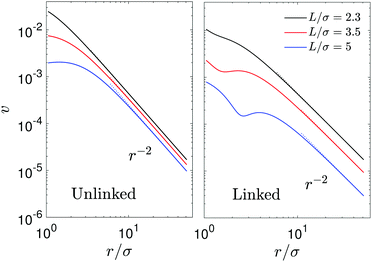 |
| | Fig. 13 The magnitude of fluid velocity,  , along the side direction (ϑ = π/2) as a function of distance r for the unlinked two spheres (left) and the linked dimer (right). The spherical polar coordinate (r, ϑ, ϕ) is taken by setting the origin of the coordinate at the middle of two spheres as in Fig. 2 and 9. The black, red, and blue lines correspond to the separation distance, L/σ = 2.3, 3.5, 5, respectively. , along the side direction (ϑ = π/2) as a function of distance r for the unlinked two spheres (left) and the linked dimer (right). The spherical polar coordinate (r, ϑ, ϕ) is taken by setting the origin of the coordinate at the middle of two spheres as in Fig. 2 and 9. The black, red, and blue lines correspond to the separation distance, L/σ = 2.3, 3.5, 5, respectively. | |
Flow field comparison
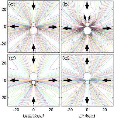
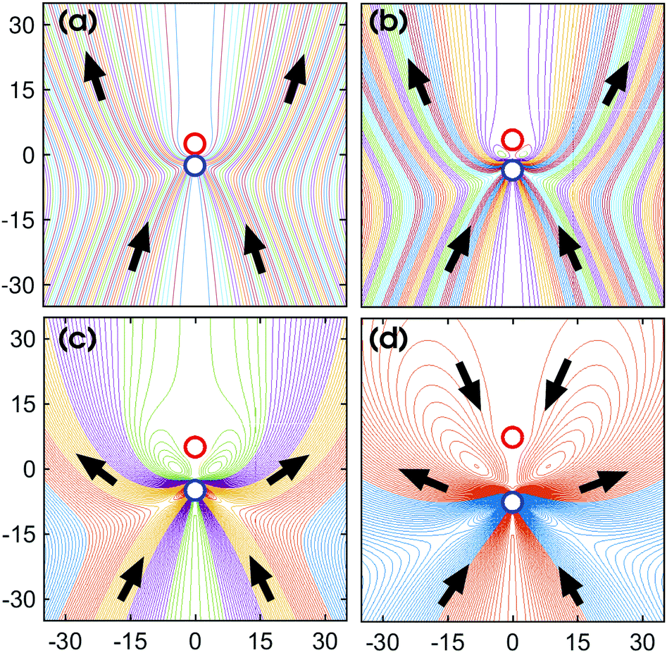
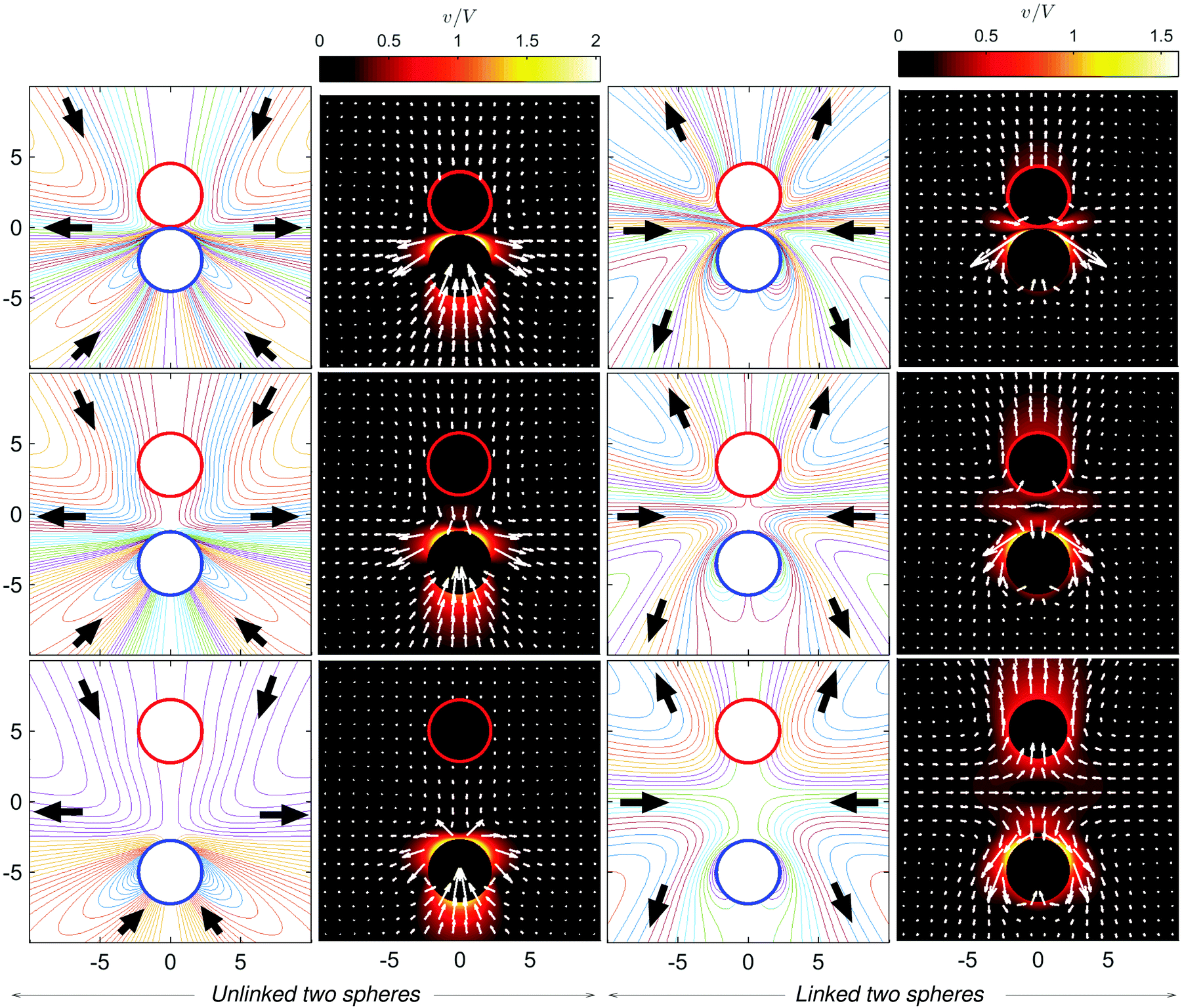
It is interesting to compare the properties of the flow fields for the freely moving catalytic and noncatalytic spheres separated by a distance L with those for a sphere-dimer with a rigid bond of length L. We refer to the spheres in the former case as unlinked spheres and those in the latter case as linked spheres. We consider the unlinked spheres to be the linked when the spheres form a dimer by self-assembly. The streamlines and flow fields just before and after the spheres self-assemble to form a sphere-dimer motor are shown in Fig. 12 (first row). It is notable that the flow directions for the unlinked spheres (first panel in this row) are completely reversed after the spheres self-assemble to form a sphere-pair (third panel in this row), although the detailed structure of the flow field changes near the S2 sphere. This implies that a sudden change in flow field occurs from a puller-like flow pattern to a pusher-like pattern.
These puller and pusher flow patterns remain unchanged as L increases (second and third rows in Fig. 12). The magnitudes of flow velocity for the unlinked and linked spheres are compared quantitatively in Fig. 13. Both cases exhibit a r−2 decay in contrast to that for a fixed S1 sphere. For small L (L/σ < 3.5), the magnitudes of flow velocity for both linked and unlinked spheres are very similar; only the flow directions have opposite signs. The asymptotic expressions are given by eqn (28) without Ω1 terms since Ω1 is zero by the force-free condition.
Sphere size effects
Lastly, we consider how the flow fields depend on ratios of the sizes of S1 and S2 spheres at the moment of dimer formation. Fig. 14 presents the streamlines for the unlinked and linked spheres near the contact distance, i.e. just before and after a dimer formation. When the S1 sphere is larger than the S2 sphere (Fig. 14(c) and (d)), the flow directions are completely reversed, except for local variations near the S2 sphere, similar to that for spheres of equal size: a puller-like flow pattern changes to a pusher-like pattern. By contrast, if the radius of the S1 sphere is smaller than that of the S2 sphere (Fig. 14(a) and (b)), the character of the far-field flow does not change and is puller-like before and after dimer formation, although the detailed structure of flow near the dimer becomes complex and exhibits several local flow circulations, especially near the S1 sphere where fluid is pushed in the direction of its head. It is interesting to note that two separated spheres with either size ratio are initially attracted and meet to form a dimer, and this dimer may have one of two counter far-field flow characteristics: either a puller or pusher depending on the size ratio.
 |
| | Fig. 14 Streamlines before and after dimer formation for different size ratios of two spheres. The left column ((a) and (c)) shows the streamlines for unlinked spheres and the right ((b) and (d)) for linked spheres. The first row ((a) and (b)) and the second ((c) and (d)) correspond to the size ratio between the S1 and S2 spheres R1/R2 = 0.5 and 2, respectively. The separation distances between spheres are L/σ = 3.5, where σ is for the small spheres, i.e. σ/a = 2. | |
6 Conclusions
Using continuum theory and particle-based simulations, a detailed study of the chemical and hydrodynamic processes that govern the dynamics of two spheres, one reactive and the other nonreactive but able to move toward high product concentrations by a diffusiophoretic mechanism, was presented in this paper. Through an analysis of the concentration and fluid flow fields the roles played by these chemical and hydrodynamic interactions could be determined. For example, when both spheres are free to move, they are attracted to each other; the nonreactive sphere moves towards the reactive sphere by diffusiophoresis while the reactive sphere is simply dragged by the flow generated by the nonreactive sphere. When the spheres are in close proximity this motion must cease; the velocity of the reactive sphere changes its sign since the nonreactive sphere now drives the pair forward by the same diffusiophoretic mechanism that operates for a sphere-dimer motor with a rigid bond. The flow field must reorganize to accommodate this change and adopts a pusher character.
The characteristics of the flow fields depend on the sphere sizes. Two separated spheres behave as a puller, regardless of their sphere size ratio, while the sphere-dimer motor that is formed can have either puller or pusher characteristics, and this does depend on the size ratio. Consequently, it should be possible to construct self-propelled dimers with either of these flow characteristics by simply manipulating the sphere sizes. This feature may be used to aid in the understanding of the collective behavior of many-sphere systems, and to provide a route to the construction of complex self-assembled structures in the laboratory.25–27
The two-sphere dynamics studied in this paper may be regarded as an elementary process that contributes to the collective dynamics of mixtures of active and passive particles28–30 and sphere dimers with non-rigid bonds. The study provides insight into the mechanisms that could lead to dynamic clusters of various types that not only move but may also fragment and reassemble. In this connection, situations not considered in this paper could be of considerable interest to investigate further. If the interactions are such that the nonreactive sphere moves to lower product concentrations, in dilute solution the two sphere will simply avoid each other. However, in more dense colloidal suspensions they will be forced to interact and lead to different active collective states, analogous to the different collective dynamics of forward and backward moving sphere dimers.53
Conflicts of interest
There are no conflicts to declare.
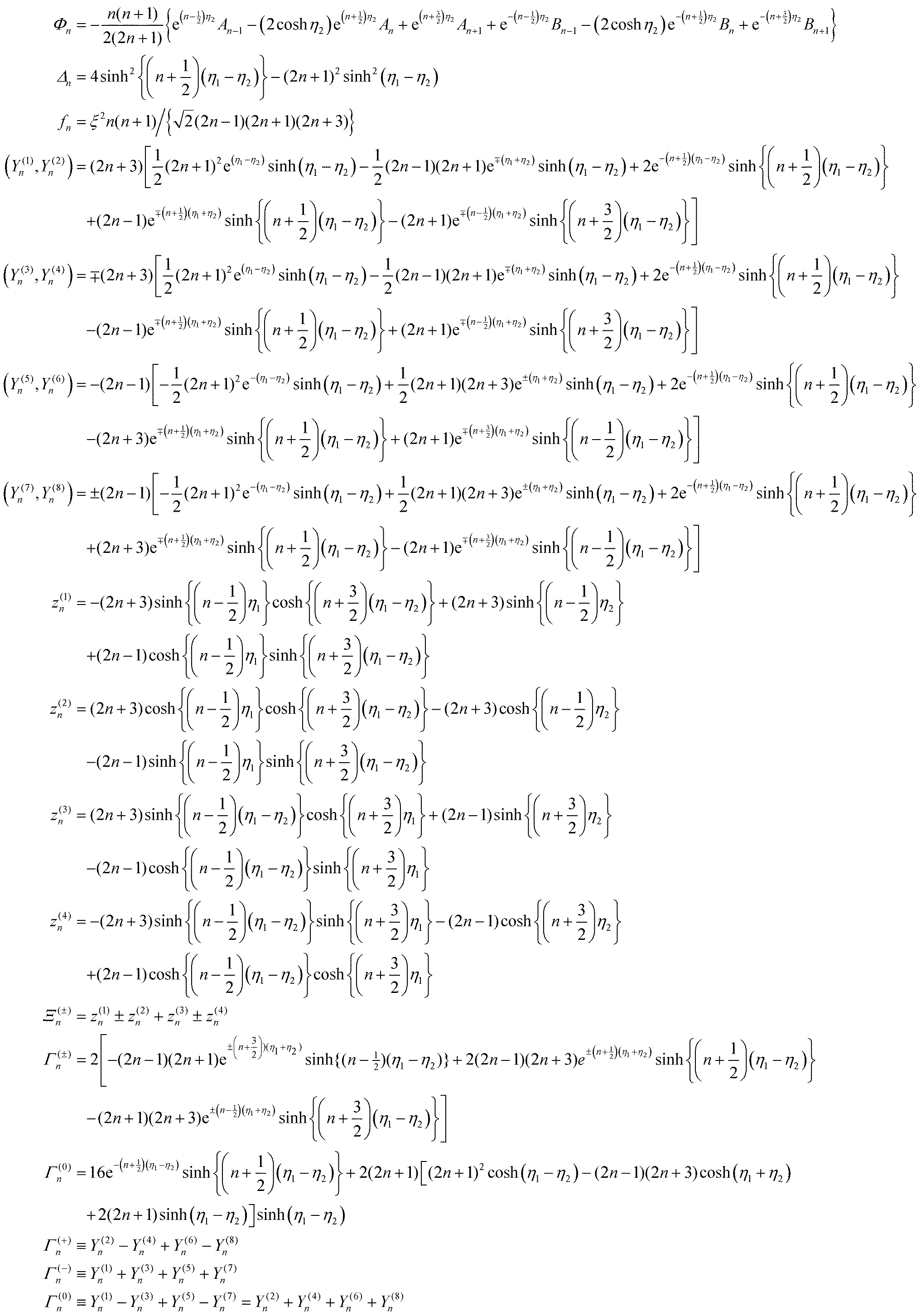
Appendix
Continuum solution information
The table in this Appendix gives the definitions of functions that enter in the continuum solution.
Table 1 The coefficients for the sphere velocity in eqn (16) and (23), and the fluid stream functions in eqn (14) and (22). The coefficients Y(o) = {Y(1)n,Y(3)n,Y(5)n,Y(7)n}, Ξ(+)n, Γ(+)n have the upper signs and Y(e) = {Y(2)n,Y(4)n,Y(6)n,Y(8)n}, Ξ(−)n, Γ(−)n have the lower signs in the equations
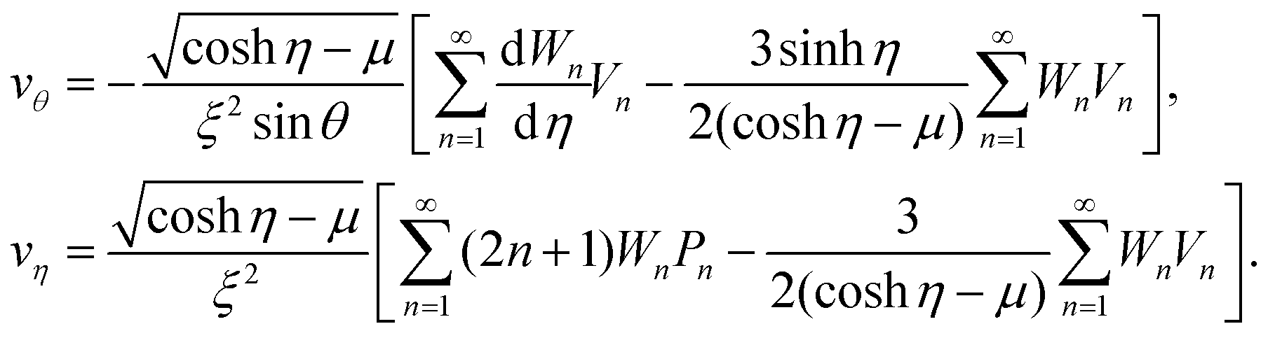
Asymptotics of fluid velocity field
Reminding the fluid velocity is given by the stream function as v = /ρ × ∇ψ, one gets the velocity components in θ and η, (vθ, vη) = {(coshη − μ)/(ρξ)}(−∂ψ/∂η, ∂ψ/∂θ) leading to| | 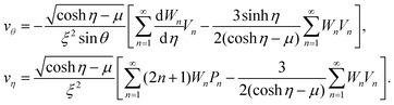 | (29) |
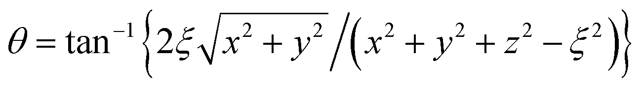
From the relations between the bispherical and Cartesian coordinates as shown in Section 2, one can show that  and η = tanh−1{2ξz/(x2 + y2 + z2 + ξ2)}. In newly introduced spherical polar coordinates (r, ϑ, ϕ) in Fig. 2, where the origin is shared, the variables θ and η in large r are approximated by Taylor series as (θ,η) ∼ (2ξ/r)(sinϑ,cosϑ) + (1/r3). Then all factors in eqn (29) are expanded by Taylor series again for large r and the final forms are expressed by eqn (28) in the main text.
Acknowledgements
S. Y. Reigh greatly thanks S. Dietrich for his support and acknowledges helpful discussion with P. Fischer in Max-Planck-Institute for Intelligent Systems. The research of RK was supported in part by a grant from the Natural Sciences and Engineering Research Council of Canada. The computational work was carried out at the HPC facility in IISER Bhopal, India. Open Access funding provided by the Max Planck Society.
References
- H. C. Berg and D. A. Brown, Nature, 1972, 239, 500–504 CrossRef PubMed.
-
H. C. Berg, E. coli in Motion, Springer, New York, 2004 Search PubMed.
- M. Eisenbach and L. C. Giojalas, Nat. Rev. Mol. Cell Biol., 2006, 7, 276–285 CrossRef PubMed.
- J. Adler, Annu. Rev. Biochem., 1975, 44, 341–356 CrossRef PubMed.
- B. V. Derjaguin, G. P. Sidorenkov, E. A. Zubashchenkov and E. V. Kiseleva, Kolloidn. Zh., 1947, 9, 335–347 Search PubMed.
-
S. S. Dukhin and B. V. Derjaguin, in Surface and Colloid Sicence, ed. E. Matijevic, Wiley, New Yok, 1974, vol. 7, p. 365 Search PubMed.
- J. L. Anderson, Ann. N. Y. Acad. Sci., 1986, 469, 166–177 CrossRef PubMed.
- J. L. Anderson, Annu. Rev. Fluid Mech., 1989, 21, 61–99 CrossRef.
- R. Golestanian, T. B. Liverpool and A. Ajdari, Phys. Rev. Lett., 2005, 94, 220801 CrossRef PubMed.
- J. R. Howse, R. A. L. Jones, A. J. Ryan, T. Gough, R. Vafabakhsh and R. Golestanian, Phys. Rev. Lett., 2007, 99, 048102 CrossRef PubMed.
- R. Kapral, J. Chem. Phys., 2013, 138, 020901 CrossRef PubMed.
- P. H. Colberg, S. Y. Reigh, B. Robertson and R. Kapral, Acc. Chem. Res., 2014, 47, 3504 CrossRef PubMed.
- Y. Hong, N. M. K. Blackman, N. D. Kopp, A. Sen and D. Velego, Phys. Rev. Lett., 2007, 99, 178103 CrossRef PubMed.
- L. Baraban, S. M. Harazim, S. Sanchez and O. G. Schmidt, Angew. Chem., Int. Ed., 2013, 52, 5552 CrossRef PubMed.
- L. Deprez and P. de Buyl, Soft Matter, 2017, 13, 3532–3543 RSC.
- J. Chen, Y. Chen and Y. Ma, Soft Matter, 2016, 12, 1876–1883 RSC.
- If the reactive sphere is subject to different interaction potentials and is diffusiophoretically active, the effects on its dynamics will be small since the concentration field in its vicinity is approximately spherically symmetric; however, at very short distances the presence of the nonreactive sphere can lead to asymmetry in the concentration field.
- G. Rückner and R. Kapral, Phys. Rev. Lett., 2007, 98, 150603 CrossRef PubMed.
- L. F. Valadares, Y.-G. Tao, N. S. Zacharia, V. Kitaev, F. Galembeck, R. Kapral and G. A. Ozin, Small, 2010, 6, 565 CrossRef PubMed.
- S. Y. Reigh and R. Kapral, Soft Matter, 2015, 11, 3149–3158 RSC.
- N. Sharifi-Mood, A. Mozaffari and U. M. Córdova-Figueroa, J. Fluid Mech., 2016, 798, 910 CrossRef.
- P. Bayati and A. Najafi, J. Chem. Phys., 2016, 144, 134901 CrossRef PubMed.
- T. Lee, M. Alarcón-Correa, C. Miksch, K. Hahn, J. G. Gibbs and P. Fischer, Nano Lett., 2014, 14, 2407 CrossRef PubMed.
- For reviews, see, R. Kapral, Adv. Chem. Phys., 2008, 140, 89 CrossRef; G. Gompper, T. Ihle, D. M. Kroll and R. G. Winkler, Adv. Polym. Sci., 2009, 221, 1 Search PubMed.
- J. Palacci, S. Sacanna, A. P. Steinberg, D. J. Pine and P. M. Chaikin, Science, 2013, 339, 936 CrossRef PubMed.
- I. Buttinoni, J. Bialké, F. Kümmel, H. Löwen, C. Bechinger and T. Speck, Phys. Rev. Lett., 2013, 110, 238301 CrossRef PubMed.
- D. P. Singh, U. Choudhury, P. Fischer and A. G. Mark, Adv. Mater., 2017, 29, 1701328 CrossRef PubMed.
- O. E. Shklyaev, H. Shum, V. V. Yashin and A. C. Balazs, Langmuir, 2017, 33, 7873–7880 CrossRef PubMed.
-
F. Schmidt, B. Liebchen, H. Löwen and G. Volpe, 2018, arXiv:1801.06868v1201.
-
T. Yu, P. Chuphal, S. Thakur, S. Y. Reigh, D. P. Singh and P. Fischer, under review.
- H. J. Keh and S. B. Chen, J. Colloid Interface Sci., 1989, 130, 542 CrossRef.
- T. Ishikawa, M. P. Simmonds and T. J. Pedley, J. Fluid Mech., 2006, 568, 119–160 CrossRef.
- M. Yang, A. Wysocki and M. Ripoll, Soft Matter, 2014, 10, 6208 RSC.
- R. Niu, D. Botin, J. Weber, A. Reinmüller and T. Palberg, Langmuir, 2017, 33, 3450 CrossRef PubMed.
- S. Ni, E. Marini, I. Buttinoni, H. Wolf and L. Isa, Soft Matter, 2017, 13, 4252 RSC.
- M. Stimson and G. B. Jeffery, Proc. R. Soc. A, 1926, 111, 110–116 CrossRef.
- M. N. Popescu, M. Tasinkevych and S. Dietrich, Europhys. Lett., 2011, 95, 28004 CrossRef.
- S. Michelin and E. Lauga, Eur. Phys. J. E: Soft Matter Biol. Phys., 2015, 38, 7 CrossRef PubMed.
- D. Papavassiliou and G. P. Alexander, J. Fluid Mech., 2017, 813, 618 CrossRef.
-
J. Happel and H. Brenner, Low Reynolds Number Hydrodynamics, Noordhoff International Publishing, 1973 Search PubMed.
-
I. Gradshteyn and I. Ryzhik, Table of integrals, Series, and Products, Academic Press, New York, 7th edn, 2007 Search PubMed.
- There is a typographical error in S. Y. Reigh and R. Kapral, Soft Matter, 2015, 11, 3149 RSC . In the coefficient
![[b with combining macron]](https://www.rsc.org/images/entities/i_char_0062_0304.gif) l in Table 1, the last component cosh(η1 + η2) should be replaced by sinh(η1 + η2). The data in the figures were computed using the correct formula.
l in Table 1, the last component cosh(η1 + η2) should be replaced by sinh(η1 + η2). The data in the figures were computed using the correct formula.
- A. Malevanets and R. Kapral, J. Chem. Phys., 1999, 110, 8605–8613 CrossRef.
- S. Y. Reigh, M.-J. Huang, J. Schofield and R. Kapral, Philos. Trans. R. Soc., A, 2016, 374, 20160140 CrossRef PubMed.
- A. Malevanets and R. Kapral, J. Chem. Phys., 2000, 112, 7260–7269 CrossRef.
- T. Ihle and D. M. Kroll, Phys. Rev. E: Stat., Nonlinear, Soft Matter Phys., 2001, 63, 020201(R) CrossRef PubMed.
- D. Sarkar, S. Thakur, Y.-G. Tao and R. Kapral, Soft Matter, 2014, 10, 9577–9584 RSC.
- T. Gao, J. Fan and Y.-G. Tao, Mol. Phys., 2016, 114, 290–296 CrossRef.
- H. A. Stone and A. D. T. Samuel, Phys. Rev. Lett., 1996, 77, 4102 CrossRef PubMed.
- A. Zöttl and H. Stark, J. Phys.: Condens. Matter, 2016, 28, 253001 CrossRef.
-
S. Kim and S. J. Karrila, Microhydrodynamics: Principles and Selected Applications, Butterworth-Heinemann, 1991 Search PubMed.
- A. A. Golovin, Int. J. Multiphase Flow, 1995, 21, 715–719 CrossRef.
- P. H. Colberg and R. Kapral, J. Chem. Phys., 2017, 147, 064910 CrossRef PubMed.
Footnote |
| † Electronic supplementary information (ESI) available: Two movies of two spheres motions, the catalytic sphere fixed in space (S1) and both spheres freely moving (S2). See DOI: 10.1039/c8sm01102h |
|
| This journal is © The Royal Society of Chemistry 2018 |
Click here to see how this site uses Cookies. View our privacy policy here. 
 Open Access Article
 This Open Access Article is licensed under a
  *a,
Prabha
Chuphal
*b,
Snigdha
Thakur
*b and
Raymond
Kapral
*a,
Prabha
Chuphal
*b,
Snigdha
Thakur
*b and
Raymond
Kapral
 ,
,  , and
, and  .
.


 in eqn (9), we can replace the boundary conditions, eqn (10) in terms of χ by
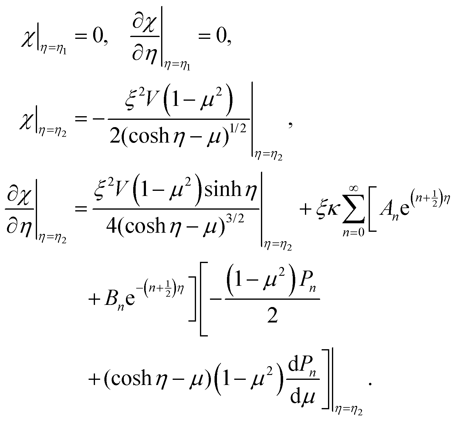
 can be expressed in a series of Legendre function Pn, (1 − μ2)Pn and μVn are rewritten by Gegenbauer functions Vn−1 and Vn+1, and (1 − μ2)dPn/dμ is rewritten by Vn.20,36,41 Then, we may expand the right sides of eqn (11) for η = η2 in a series of Vn as
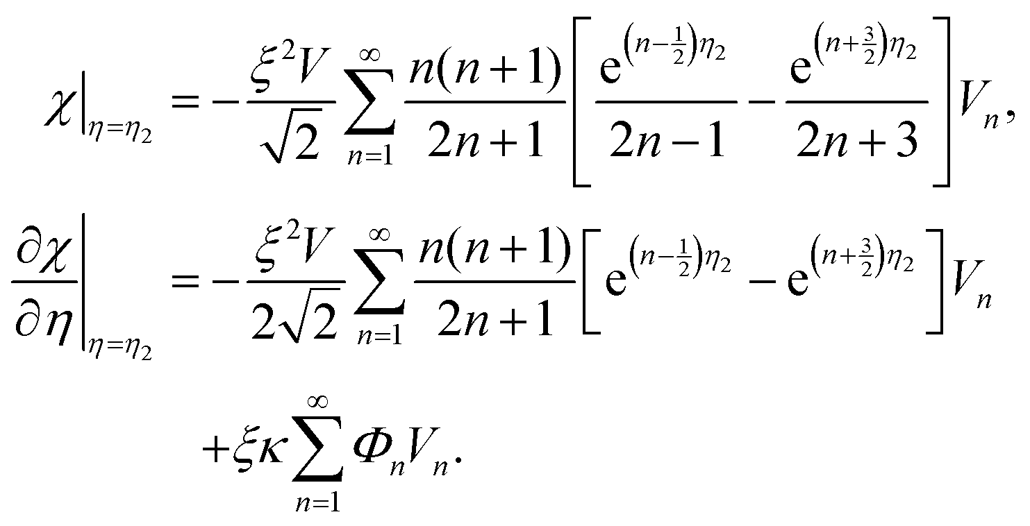
 (i = 1, 2), where Πi,z = ẑ·Πi and Π is the stress tensor. The system is symmetric around the azimuthal angle ϕ and only the force in the z-direction needs to be considered. The analytic expressions for the force exerted on the spheres by the fluid are given in Stimson and Jeffery36 as
 by
by
 is the center-of-mass velocity of the particles in the cell to which the particle i belongs, and Nc is the number of particles in that cell. A random shift of the collision lattice is applied at every collision step to ensure Galilean invariance.46 The dynamics locally conserves mass, momentum and energy.24
 , respectively. The cubic simulation box with linear dimension Lb = 50 and periodic boundary conditions in all dimensions is divided into Lb3 = 503 cubic cells. Multiparticle collisions are carried out in each cell by performing velocity rotations by an angle α = 120° about a randomly chosen axis every collision time h = 0.1. The average solvent number density is c0 = 10 and the temperature is kBT = 1. The MD time step is Δt = 0.01. The energy parameters for the S2 sphere-fluid repulsive LJ potentials are εA = 1.0 and εB = 0.1 for A and B, respectively, while εA = εB = 1.0 for the S1 sphere. The size parameters are σ = 2 and σs = 4 to give effective sphere radii of R1 = R2 = 21/6σ. The sphere mass is taken to be M = 4πσ3c0/3 corresponding to neutral buoyancy. The intrinsic reaction rate constant for the A + S1 → B + S1 reaction can be estimated from simple collision theory so that
  . The transport properties of the fluid depend on h, α, and Nc. The fluid viscosity is
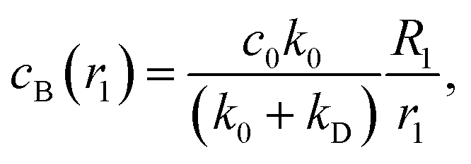
 ,20 where a new spherical polar coordinate (r, ϑ, ϕ) in Fig. 2 is chosen sharing the origin, by taking the limit of η2 → −∞ (R2 → 0) and L → ∞ and noting that the n = 0 term is sufficient.
 , are presented. The first, second, third rows are for L/σ = 2.5, 3.5, 5. In the color maps, the magnitude of the fluid velocity v is scaled by the sphere velocity V, where V = 0.053, 0.023, 0.011 for L/σ = 2.5, 3.5,5, respectively. The red and blue circles indicate the S1 catalytic and S2 noncatalytic spheres.
 , where v = vθ
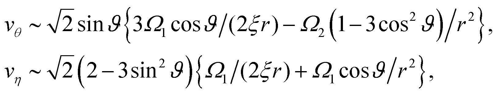
 and
and  . The details are given in the Appendix.
 , for ϑ = π/2 as a function of distance r, where the spherical polar coordinates (r, ϑ, ϕ) are taken with a common origin in Fig. 2. The black, red, green, blue, brown, magenta lines (from top to bottom) correspond to the separation distances, L/σ = 2.5, 3.5, 5, 7.5, 10, 15, respectively.
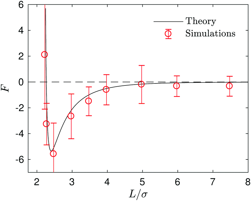

 , along the side direction (ϑ = π/2) as a function of distance r for the unlinked two spheres (left) and the linked dimer (right). The spherical polar coordinate (r, ϑ, ϕ) is taken by setting the origin of the coordinate at the middle of two spheres as in Fig. 2 and 9. The black, red, and blue lines correspond to the separation distance, L/σ = 2.3, 3.5, 5, respectively.
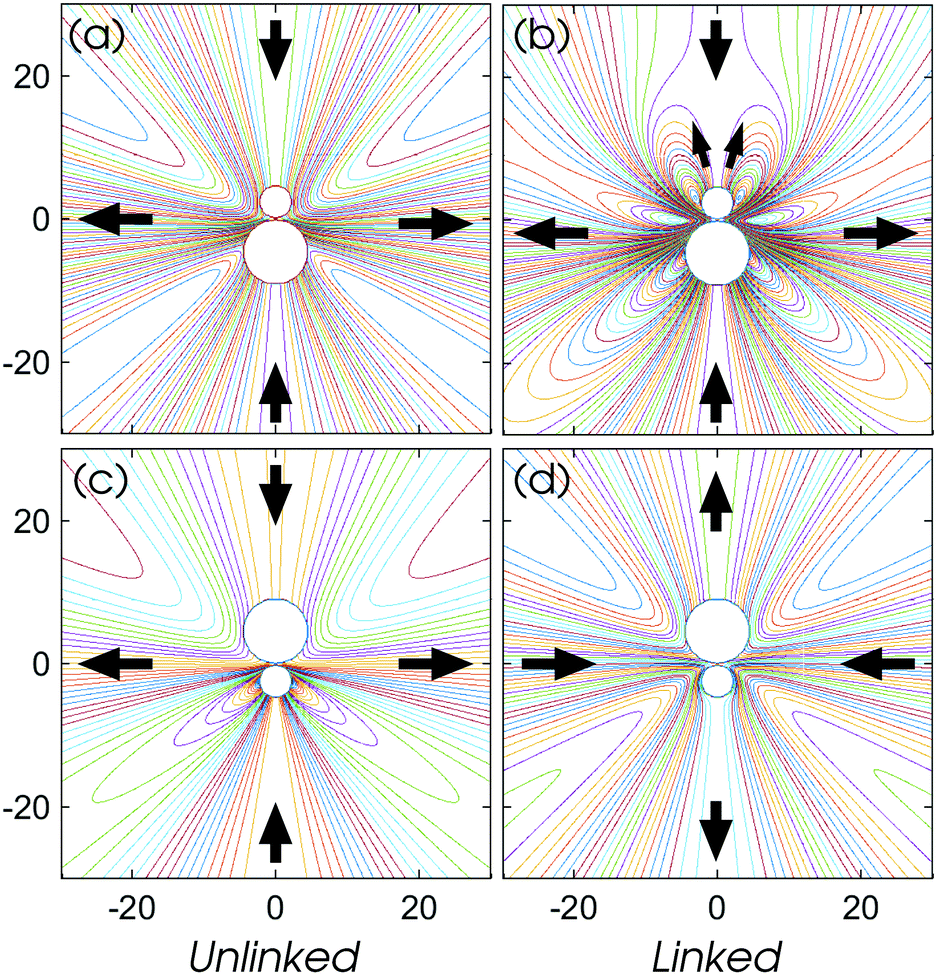
 and η = tanh−1{2ξz/(x2 + y2 + z2 + ξ2)}. In newly introduced spherical polar coordinates (r, ϑ, ϕ) in Fig. 2, where the origin is shared, the variables θ and η in large r are approximated by Taylor series as (θ,η) ∼ (2ξ/r)(sin