
 Open Access Article
 This Open Access Article is licensed under a
 Creative Commons Attribution 3.0 Unported Licence
Osmotic pressure in polyelectrolyte solutions: cell-model and bulk simulations
Magnus
Ullner
 *a,
Khawla
Qamhieh
b and
Bernard
Cabane
c
*a,
Khawla
Qamhieh
b and
Bernard
Cabane
c
aTheoretical Chemistry, Lund University, POB 124, SE-221 00 Lund, Sweden. E-mail: magnus.ullner@teokem.lu.se
bPhysics Department, College of Science and Technology, Al-Quds University, Jerusalem, Palestine
cLaboratoire PMMH, ESPCI, 10 Rue Vauquelin, 75231 Paris cedex 5, France
First published on 22nd June 2018
Abstract
The osmotic pressure of polyelectrolyte solutions as a function of concentration has been calculated by Monte Carlo simulations of a spherical cell model and by molecular dynamics simulations with periodic boundary conditions. The results for the coarse-grained polyelectrolyte model are in good agreement with experimental results for sodium polyacrylate and the cell model is validated by the bulk simulations. The cell model offers an alternative perspective on osmotic pressure and also forms a direct link to even simpler models in the form of the Poisson–Boltzmann approximation applied to cylindrical and spherical geometries. As a result, the non-monotonic behaviour of the osmotic coefficient seen in simulated salt-free solutions is shown not to rely on a transition between a dilute and semi-dilute regime, as is often suggested when the polyion is modelled as a linear flexible chain. The non-monotonic behaviour is better described as the combination of a finite-size effect and a double-layer effect. Parameters that represent the linear nature of the polyion, including an alternative to monomer concentration, make it possible to display a generalised behaviour of equivalent chains, at least at low concentrations. At high concentrations, local interactions become significant and the exact details of the model become important. The effects of added salt are also discussed and one conclusion is that the empirical additivity rule, treating the contributions from the polyelectrolyte and any salt separately, is a reasonable approximation, which justifies the study of salt-free solutions.
1 Introduction
The osmotic pressure of a solution measures its ability to gain or retain solvent molecules in an exchange with the surroundings, i.e., the chemical potential of the solvent. To a first approximation, in an ideal solution, the origin of the effect is the entropy of mixing and the osmotic pressure is proportional to the total concentration of solutes. A dissociated polyelectrolyte consists of a charged polymer and its n counterions, thus, giving a n + 1 times larger contribution than a neutral polymer. However, in a real solution, there are attractive interactions between the polyion chain and the counterions, which lower the osmotic pressure. The deviation from the ideal pressure is expressed by the osmotic coefficient, which is the ratio between the real osmotic pressure and the ideal pressure.The osmotic pressure is at the origin of the exceptional swelling of polyelectrolyte gels, which can swell in water to volumes that are 1000 times that of the dry polymer. It is used in superabsorbants (polyelectrolyte gels for baby diapers and for gardening) and in microgels (thickeners for cosmetics and creams for personal care). In the latter case, retaining most of the available water makes it possible to obtain the desired rheological properties, i.e., gels that are not sticky and will release water under applied pressure. It is also an important property for food gels, which must have a well-controlled behaviour in the swollen state. In the human body, the water-retaining properties of polyelectrolytes can be found in the vitreous body of the eye and in synovial joint fluid.
Most of these applications involve the swelling of a gel in an aqueous solution that contains various electrolytes. This swelling is a result of the difference between the osmotic pressure of the gel and that of the surrounding solution. The practical problem is then to maintain a high net pressure in gels equilibrated with a solution at significant ionic concentration. This situation is reproduced in experimental setups where the polyelectrolyte solution is contained by a semipermeable membrane that allows solvent, small ions and other small solutes to pass through, but not polymers. In such situations the measured pressure difference is not between the polyelectrolyte solution and pure solvent (zero osmotic pressure), but between this solution and a reference solution, which may contain salt, on the other side of the membrane. To characterise the solution in terms of osmotic pressure, there is then a choice between quoting the measured pressure difference or recalculating the value as for the equilibrium with the pure solvent. We will use the term net osmotic pressure for the pressure difference between a polyelectrolyte solution and a salt solution and the osmotic pressure with respect to pure solvent will be called absolute osmotic pressure.
Various experimental techniques have been used to measure the osmotic pressure/coefficient of polyelectrolyte solutions in the past. In the isopiestic method,1,2 the liquid phases of the sample and a reference solution with a known equation of state (osmotic pressure as a function of concentration), for example, a solution of KCl, are kept separate and the equilibrium for the solvent water is established via its vapor phase. The equilibrium concentration of the reference solution gives the absolute pressure of the sample.
Most other techniques separate two liquid phases by a semipermeable membrane as described above, which means that the reported osmotic pressure corresponds to an absolute pressure if there is no salt present. Otherwise, it is a net pressure. Osmotic pressure can be measured directly as a pressure difference between the sample compartment and a compartment with pure solvent or an electrolyte solution (osmotic pressure method). In the osmotic concentration method,3 a reference solution is used in a similar fashion to the isopiestic method, although the reference is a neutral polymer, typically polyethylene glycol (PEG), since it should not be able to enter the sample solution through the membrane. The equilibrium concentration is interpolated to a concentration where there is no volume change between compartments. Using a polymer solution of known osmotic pressure is more generally known as the osmotic stress method. It can also be used to force the sample solution to adopt ordered structures and does not always require a membrane.4 The experiments that we will refer to as osmotic stress measurements used a PEG solution as the external reference and the sample compartment was a dialysis bag.5
To gain additional insight, the osmotic pressure of polyelectrolyte solutions have also been calculated by simulations for both flexible and stiff chains.6–19 Most studies have been for salt-free systems, but some have considered the effects of added salt.16,18,19 It is generally argued that the counterions give the main contribution to the osmotic pressure from the polyelectrolyte, but Chang and Yethiraj took a different view when they focused on the excess part of the osmotic coefficient and stressed the importance of the polyion–counterion interactions in a salt-free system14 and also pointed to non-negligible polymer–polymer contributions in a study including salt.19
Comparisons to experimental values have been made for simulations of stiff chains and a general trend is that the simulations give higher values of the osmotic coefficient.6,10,12,16 The difference is not always large and can sometimes be removed by adjusting the simulation parameters,12 but Antypov and Holm got significantly higher values, which could not be explained by any known deficiency of the model.16 Arh et al. showed that for various experimentally measured polyelectrolytes, the osmotic coefficient does not approach 1 as the linear charge density goes to zero; i.e., there is a contribution to the non-ideality that is not due to electrostatic interactions.
The simplest possible description of a polyelectrolyte solution is a cell model,20–23 where the solution is treated as independent cells, each containing one chain with neutralising counterions and salt, if present. It is attractive, because, computational benefits aside, it allows us to focus on the interactions between the polyion and the ions, which dominate the polyelectrolyte effect on osmotic pressure. Thus, we use the simplicity of the cell model to get a better understanding of the system. To this end, we have performed Monte Carlo simulations of a flexible, coarse-grained polyion and simple ions to obtain osmotic pressures and osmotic coefficients as functions of the monomer concentration. However, we have also performed molecular dynamics simulations with multiple chains and periodic boundary conditions to validate the cell-model simulations as well as to obtain results free of the artefacts that do exist in the cell model.
After describing the model and simulation details, the discussion of the results will start with a comparison to experiments to establish that the basic model is relevant, followed by a comparison between bulk simulations and cell-model simulations to establish that we can use the cell model as a pedagogical tool. Then we look more closely at the inner workings of the system in the form of particle distributions and the mechanisms behind a non-monotonic osmotic coefficient. We also explore the use of an alternative set of parameters that reflect the linear nature of the polyions. The main discussion is based on salt-free cases, which is justified in a discussion of the effects of adding salt.
2 Simulations
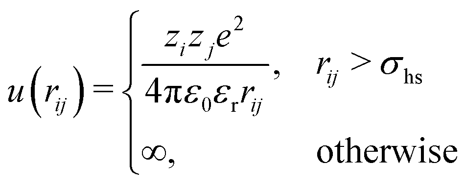
We have performed molecular dynamics simulations of a bulk system of salt-free polyelectrolytes contained in a cubic box with periodic boundary conditions in the NPT ensemble using the software package GROMACS (versions 4.5.4 and 4.5.5).24–26 We have also performed Monte Carlo simulations of a cell model,22,23,27 which means that the polyelectrolyte solution is viewed as independent cells, i.e., closed volumes with no interactions across the boundaries. Normally, each cell contains only one chain with neutralising counterions and salt. The size of the cell, which is taken to be spherical with a radius Rcell, then determines the monomer concentration, cm. The Monte Carlo simulations were canonical with respect to the polyion and its counterions and grand canonical with respect to salt, if present. As a schematic representation, snapshots from the two types of systems can be found in Fig. 1.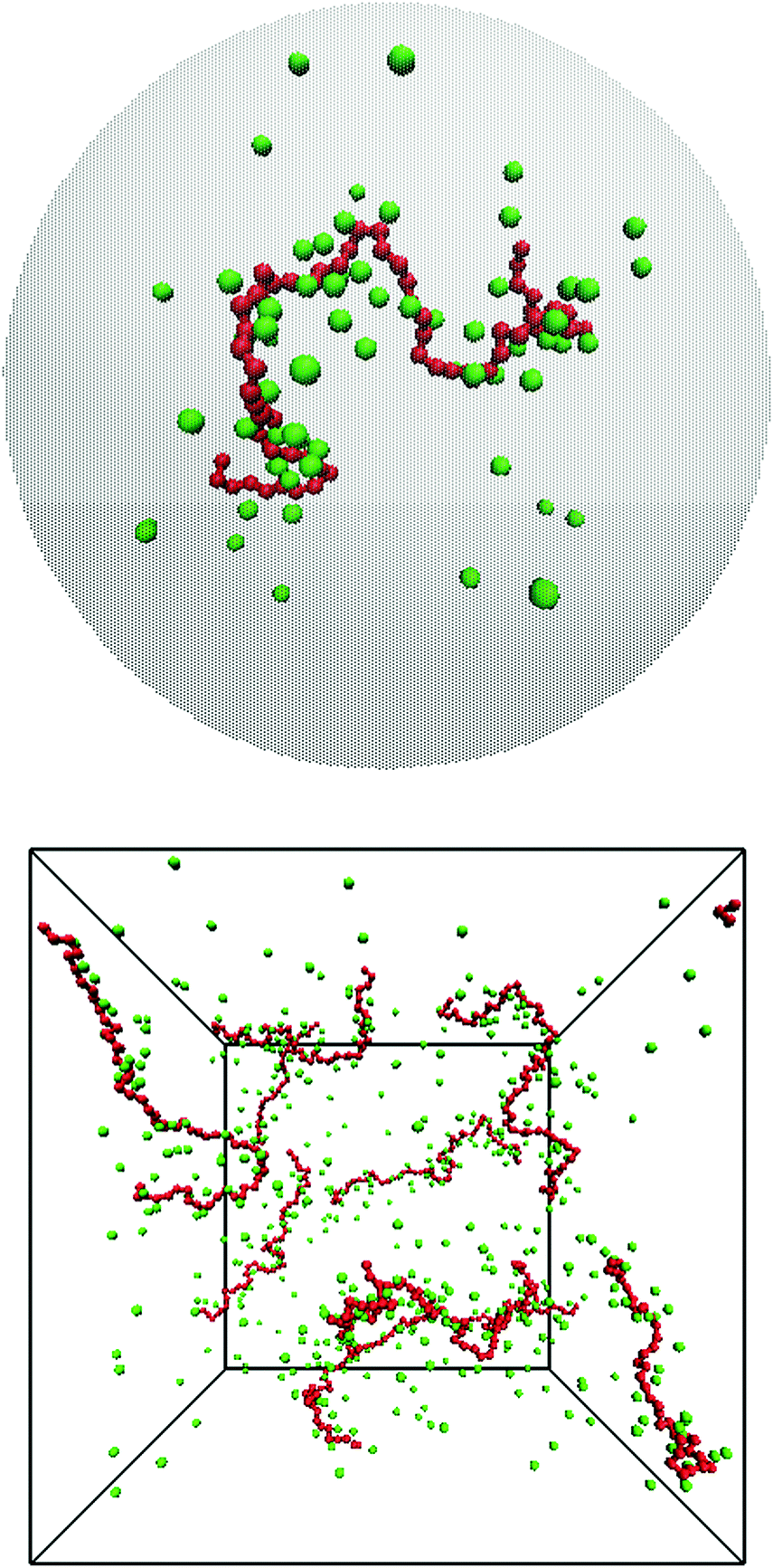 | ||
| Fig. 1 In this work, polyelectrolyte solutions are typically simulated as either a single freely jointed chain of charged hard spheres (red) with neutralising counterions (green) confined in a spherical cell with radius Rcell (top) or eight such polyelectrolytes in a cubic box with periodic boundary conditions (bottom). The examples show snapshots of fully charged (α = 1.0) salt-free 64mers with bond length b = 4.5 Å and a monomer concentration of 0.074 M. | ||
We modelled the polyion as a set of N charged spheres connected by rigid bonds (rigid in the Monte Carlo simulations, harmonic with a very large force constant in the molecular dynamics simulations). There was no angular potential; i.e., the chains were freely jointed. A polyion is denoted as an Nmer, e.g., a 64mer has N = 64 monomers. Depending on the context, chain size will either refer to the number of monomers or the contour length, L = bN, where b is the bond length. The polyion was neutralised by monovalent spherical ions and the system could also contain positive and negative monovalent salt ions. The electrostatic interactions in the system were described in the primitive model, where the solvent (water) is treated as a structureless dielectric continuum with a dielectric constant, εr = 78.7. The coarse-grained polymer model means a dramatic decrease of the number of interaction sites compared to an atomistic model.
In the Monte Carlo simulations, monomers and ions were represented as hard spheres with a hard-core diameter σhs = 4 Å. Formally we can write the interactions in the system as,
 | (1) |
To be able to calculate forces in the molecular dynamics simulations, a truncated and shifted Lennard-Jones potential was used instead of hard spheres to represent the size of monomers and ions,
 | (2) |
The cell-model simulations followed standard procedures with pivot, crankshaft, and centre-of-mass moves for the polymer and single particle moves for the ions.28–31 The absolute osmotic pressures were calculated from the particle concentrations (monomers and ions) at the cell boundary according to the contact theorem,23,32
| Πabs = RTΣci(Rcell) | (3) |
| Πnet = Πabs − Πref | (4) |
Deviations from the ideal osmotic pressure can be represented by the osmotic coefficient
 | (5) |
With (1![[thin space (1/6-em)]](https://www.rsc.org/images/entities/char_2009.gif) :1) salt present, there are also co-ions with a concentration c2 and electroneutrality means that the counterion concentration in the cell is c1 = (αcm + c2). In principle, the ideal pressure in a cell is given by the actual concentrations, but in a salt equilibrium, the distribution of ions between the cell and the reference solution is determined by interactions and the measured concentrations are therefore not ideal in themselves. Instead, an estimate of the ion distribution and the ideal pressure can be obtained through a Donnan equilibrium that assumes ideal conditions everywhere35
:1) salt present, there are also co-ions with a concentration c2 and electroneutrality means that the counterion concentration in the cell is c1 = (αcm + c2). In principle, the ideal pressure in a cell is given by the actual concentrations, but in a salt equilibrium, the distribution of ions between the cell and the reference solution is determined by interactions and the measured concentrations are therefore not ideal in themselves. Instead, an estimate of the ion distribution and the ideal pressure can be obtained through a Donnan equilibrium that assumes ideal conditions everywhere35
| c1c2 = cref1cref2 = cs2 | (6) |
 | (7) |
 | (8) |
Rather than using the full ideal pressure as given above, the osmotic coefficient is often used to compare the osmotic pressure to the ideal contribution from only the polyelectrolyte, i.e., the polyion and its own counterions,
 | (9) |
3 Results and discussion
3.1 Comparison to experiments
Table 1 lists some details of experimental studies on solutions of sodium polyacrylate and Fig. 2 shows a comparison between the osmotic coefficients for the salt-free cases with a high degree of ionisation. Most of the long chains give similar values of the osmotic coefficient. A notable exception is the case of osmotic stress measurements (N = 375),5 which gives significantly lower values. This could possibly be due to the equation of state used for the osmotic pressure of the reference PEG solution. Another data set that stands out is the isopiestic measurements for N = 640,39 with higher values than the apparent consensus of the other long chains.| N | c s/M | Method (reference compound) | Source |
|---|---|---|---|
| 13 | 0 | Isopiestic (KCl) | Zhang et al.36 |
| 340 | 0 | Osmotic pressure | Kern37 |
| 375 | 0; 5 × 10⁻³–0.12 | Osmotic stress (PEG) | Pochard et al.5 |
| 600 | 0; 2 × 10⁻⁴–1 | Osmotic concentration (PEG) | Alexandrowicz38 |
| 640 | 0 | Isopiestic (KCl) | Asai et al.39 |
| 1640 | 0 | Isopiestic (KCl) | Ise and Okubo1 |
| 3600 | 0 | Osmotic concentration (PEG) | Alexandrowicz40 |
| 3600 | 0 | Osmotic pressure | Kakehashi et al.41 |
| 9000 | 0.1 | Osmotic pressure | Orofino42 |
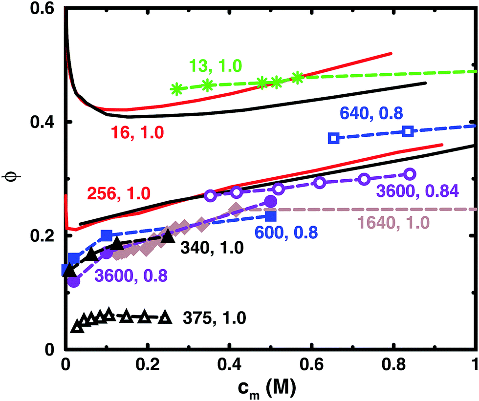 | ||
| Fig. 2 Osmotic coefficients for salt-free solutions taken from experiments (dashed lines with symbols) and simulations (solid lines without symbols). Simulations were performed with 8 chains in a cubic box with periodic boundary conditions (black solid lines) and with a single chain in a spherical cell (red solid lines). The bond length used in the simulations ([N = 16, α = 1.0] and [N = 256, α = 1.0]) was 2.52 Å. The experiments are results for sodium polyacrylate with a high degree of ionisation: [N = 13, α = 1.0] (green stars);36 [N = 340, α = 1.0] (black filled triangles);37 [N = 375, α = 1.0] (black open triangles);5 [N = 600, α = 0.8] (blue filled squares);38 [N = 640, α = 0.8] (blue open squares);39 [N = 1640, α = 1.0] (brown filled diamonds);1 [N = 3600, α = 0.8] (purple filled circles);40 [N = 3600, α = 0.84] (purple open circles).41 For experimental methods, see Table 1. Note that chains with similar lengths have the same colour and shape of the symbol. The lines are just connecting the data points and some points are outside the displayed range of concentrations. | ||
Thus, if we regard the measurements for N = 375 and 640 as outliers, the experimental results confirm the old conclusion that for sufficiently long polyions, the osmotic coefficient is independent of molecular weight.43 Below we will show that this also applies to the simulated chains.
The figure also contains curves obtained from simulations using a bond length of 2.52 Å, which corresponds to the charge separation along the backbone of polyacrylate. Overall, the agreement between the simulations and the experimental data is remarkably good considering the simplicity of the model. The single-chain cell model gives a larger slope at higher concentrations than the corresponding simulation of 8 chains in a periodic box for a 16mer, but the two simulation approaches give more or less the same result for a 256mer, which is beyond the long-chain limit of the simulations (see Section 3.5). Considering this limit, our simulations can be said to confirm the general conclusion that simulations give higher values of the osmotic coefficient than experiments,6,10,12,16 as discussed in the Introduction.
Looking more closely at the simulated and experimental curves, a noteworthy difference is that they have opposite trends at the lowest concentrations. The experimental osmotic coefficients show a fast (compared to the slope at higher concentrations) increase with concentration, starting from a low value, whereas the simulation results display a fast decrease from the ideal value. It can be argued that the longer experimental chains are too long to show the initial decrease at the observed concentrations, but it is likely that the value at high dilution is indeed low. This is because the ionic strength of real “pure water” is not zero and the membrane techniques can be expected to show results similar to simulations with low concentrations of added salt; i.e., the osmotic coefficient should tend to zero when the polyelectrolyte is highly diluted (see below), as has been discussed and demonstrated by Antypov and Holm.16 However, there is also a tendency for the longest simulated chains to show a dip just before the increase in the osmotic coefficient as the concentration is reduced. This may be a manifestation of the chain being very elongated and having approximately cylindrical symmetry, because, as will be shown later, a Poisson–Boltzmann calculation for an infinite cylinder shows a similar feature. The mechanisms behind the non-monotonic behaviour of the simulations is discussed in Section 3.4.
Another difference is that the simulations tend to show a somewhat stronger increase of the osmotic coefficient at higher concentrations than the experiments, but it depends on which curves we compare and we should perhaps not ask too much of the coarse-grained model. Thus, given the experimental uncertainties and the simplified nature of the model, we are content that there is good agreement and will focus on the trends rather than the quantitative results.
The charge separation along the backbone of polyacrylate, 2.52 Å, was used as a bond length. Previously, the cell model has given a good agreement with the titration curve of polyacrylic acid using a bond length of 4.5 Å.44 This gives a larger osmotic coefficient. Thus, selecting the smaller bond length improves the agreement with experiments here at the cost of being inconsistent. However, it may also be an illustration of the point that there are many different length scales in a polyelectrolyte system and it is difficult to capture everything with a few parameters. In the case of titration vs. osmotic pressure, the leading interaction terms are different, intramolecular polyion interactions and polyion–ion interactions, respectively, and it could be argued that the former is best described by the separation between neighbouring charges, which is longer than the projected distance along the backbone, because the charges reside on side chains in a real polyacrylate, whereas in the case of the osmotic pressure, the projected distance could be more significant, since this is the linear charge density experienced by the counterions not in the immediate vicinity of the chain. Other length scales in the system are the chain extensions and the ion distributions, which are interconnected.
3.2 Single vs. multiple chains
Fig. 3 and 4 compare the results from simulations with different numbers of polyions.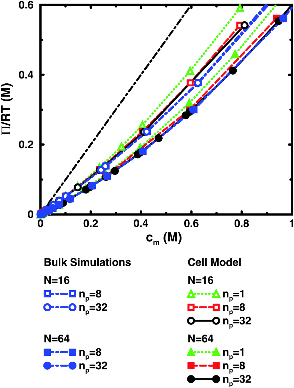 | ||
| Fig. 3 Osmotic pressure as a function of monomer concentration for salt-free simulations of 16mers (open symbols) and 64mers (filled symbols) with 8 (squares, blue dot-dashed lines) and 32 (circles, blue dot-dashed lines) polyions in a cubic box with periodic boundary conditions as well as simulations of 1 (triangles, green dotted lines), 8 (squares, red dashed lines), and 32 (circles, black solid lines) polyions in a spherical cell. The bond length is b = 4.5 Å and the degree of ionisation is α = 1. The black dot-dashed line without symbols shows y = x, which corresponds to the ideal pressure if the polyion contribution is neglected. | ||
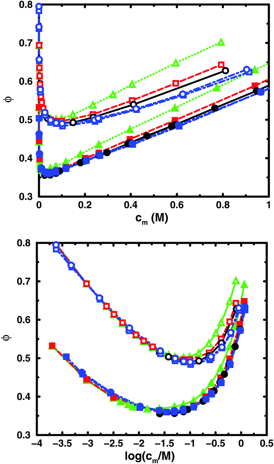 | ||
| Fig. 4 Osmotic coefficient as a function of monomer concentration (linear scale top, logarithmic scale bottom) for the same cases as in Fig. 3. | ||
In the bulk simulations with periodic boundary conditions, it makes practically no difference if the box contains 8 or 32 chains, which shows that very few polyions are needed to describe the osmotic pressure.
The normal cell model takes the reduction of chains to the extreme by focusing on a volume containing a single polyion. At high concentrations, the size and shape of the cell limits the extension of the polyion. This is partly a real effect, since the surrounding chains have a confining effect and the hard cell boundary and its spherical shape approximate this effect. The approximation is expected to deteriorate with increasing monomer concentration. High salt concentrations limit the chain expansion and will improve the approximation. Supporting evidence for the cell model as such is that it seems to be an excellent approximation for charged spherical colloids like silica and latex particles.45
To check how the confinement affects the results, an extended cell model was used with more than one chain in a larger cell, still with no interactions across the spherical boundary as for the normal cell model with a single chain and with the pressure obtained from the concentrations on the boundary. At low concentrations, the osmotic pressures are the same, while at high concentrations, a single chain gives a slightly higher pressure, because the spherical boundary does congest the conformations of a single chain. Looking at the osmotic coefficient, we see different slopes for single and multiple chains at high concentrations. On the other hand, the difference between 8 and 32 polyions in a cell is small. For the 64mer, 32 chains are in excellent agreement with the bulk simulations, while the confinement effect is still visible for 32 16mers. This shows that the cell-model simulations give osmotic pressures that quickly approach bulk values, even at the higher concentrations, as the number and the size of the chains increase.
Fig. 5, displaying 64mers with two different bond lengths and three degrees of ionisation, further illustrates that the cell model shows the same trends as the bulk simulations, albeit with the artefact of somewhat higher osmotic coefficients at the higher concentrations.
 | ||
| Fig. 5 Osmotic coefficient as a function of monomer concentration in salt-free cell-model simulations (top) and bulk simulations (bottom) of 64mers with bond lengths b = 3 Å (filled symbols, black solid lines) and 6 Å (open symbols, red dashed lines) and with α = 0.25 (triangles), 0.5 (squares), and 1 (circles). The trends are the same, although the cell-model simulations give somewhat higher osmotic coefficients than the bulk simulations at high concentrations. | ||
The main conclusion here is that the osmotic pressure of a single chain in a cell shows the same qualitative features as multiple chains in bulk simulations. The advantage of the single-chain cell model is that it represents a simpler system than the bulk system and since the osmotic pressure is obtained from the concentrations on the boundary, insight can be gained by looking for mechanisms that affect these concentrations, in contrast to discussing force balances in the bulk. It also forms a link to even more simplified cell models in the form of solutions to the Poisson–Boltzmann equation, which make it possible to investigate purely electrostatic effects.
3.3 Particle distributions
Since the concentrations at the boundary give the osmotic pressure in a cell model, the polyelectrolyte effect can be visualised through the distributions of monomers and ions in the cell. Fig. 6 shows the distributions from a single-chain simulation without salt. | ||
| Fig. 6 Monomer (black solid line) and ion (red dashed line) distributions in simulations of a single 64mer (b = 4.5 Å and α = 1) without added salt in a cell with a radius of 70 Å (cm = 0.074 M). The statistics grow poor for the concentrations towards the centre of the cell (r → 0), because the sampled volume becomes small. The concentrations at the cell radius show the contributions from monomers and ions to the osmotic pressure. The dot-dashed line shows their average concentrations (the ideal counterion pressure). | ||
The distributions show that the osmotic pressure (the total concentration c at r = Rcell) is dominated by the counterions. This is natural in a classical view, where the polyion is counted as one, while the counterions are counted separately, which means that the latter would dominate by their larger number. In the cell model, the monomers are counted separately, but the effect is the same, because the polyion conformations span a volume that prevents more than a few monomers to reach the boundary at the same time (most monomers are inside this volume and only part of its surface can touch the boundary at one time). This is true for the ideal system as well as for the charged system.
In the polyelectrolyte system, the effect of the chain connectivity of the polyion is to bring charges close together to give a locally high charge density. The counterions are attracted to the polyion and establish an electrical double layer, which is partly inside the polymer domain and partly extends out from it, as indicated by the similarities of the monomer and counterion distributions in the figure. The result is that the counterion concentration at the boundary is lower than the average counterion concentration in the cell and the osmotic pressure is lower than the ideal value. Thus, the polyelectrolyte effect is a correlation between the polyion and the counterions that reduces the osmotic pressure.
At low concentrations, the polyion prefers to be distributed around the centre of the cell to retain a fairly symmetrical ion atmosphere. At higher concentrations, the maximum of the monomer distribution moves off-centre, as shown in Fig. 6. This is an artefact due to the combined effect of the confinement and the intrachain repulsion. When the latter extends the chain and conformations that maximise the end-to-end distance do not fit in the spherical cell, the chain can still be extended and unhindered over a short to medium range by tracing spherical shells. A long, semi-flexible chain would tend to line the inner wall of a small spherical cavity, to minimise the bending of the chain, such as the case of DNA inside a viral capsid, but with the polyion, keeping the local symmetry of the ion atmosphere prevents the chain from getting too close to the boundary. Thus, the figure also shows that, although the confinement affects the monomer distribution, monomers do not necessarily contribute much to the concentration at the boundary, i.e., the osmotic pressure. In other words, there is a limit to how much the diffuse part of the double layer can be compressed and how much the positive and negative charge distributions can be offset with respect to each other, which excludes chains from the boundary. In the bulk, this would translate to chains avoiding each other through a double-layer repulsion.
3.4 Non-monotonic osmotic coefficient
Fig. 4 and 5 display the typical non-monotonic behaviour for simulations of (perfectly) salt-free solutions of finite chains with an osmotic coefficient that is decreasing at low polyelectrolyte concentrations and increasing at higher concentrations as the concentration increases.7,9,13–16 At extremely low concentrations, the counterions are diluted away from the polyion (and each other), making interactions negligible, and the system approaches ideal behaviour with ϕ = 1 when the concentration is decreased. The counterion distribution is a trade-off between a low electrostatic energy in the neighbourhood of the polyion and the entropic driving force to spread the ions in the cell. At low concentrations, increasing the concentration reduces the entropic part by decreasing the available volume, while the average polyion–counterion interaction becomes stronger. The correlations between the counterions and the polyion reduce the effective counterion concentration (concentration at the boundary in the cell model) and ϕ decreases.The non-monotonic behaviour of the osmotic coefficient (or the corresponding behaviour of the osmotic pressure) is often discussed in relation to a transition between a dilute and a semi-dilute regime.9,13,14 The transition occurs at the so-called overlap concentration, where the average monomer concentration of the solution reaches the same concentration as in the polymer domain. In the semi-dilute regime, it is no longer relevant to discuss the interactions of individual chains and it is better to regard chain segments of a certain correlation length as the interacting units contributing to the pressure of the system, as in various scaling theories.46–48
Liao et al. could couple the minimum between the two regimes to the overlap concentration for long chains (N ≥ 187),13 but many cases show a minimum below the overlap concentration13,14 and for the shortest chain (N = 25), Liao et al. found the minimum at a concentration 8 times smaller than the overlap concentration. Thus, there is no apparent universal connection between the minimum and the overlap concentration and using the measured chain extension (radius of gyration or root-mean-square end-to-end distance) to gauge the volume of the polyion domain, our data do not show any consistent correlation, either.
There are a number of problems with using the concept of overlap concentration and the semi-dilute regime. First, the overlap concentration itself is a conceptual construct, labelling the crossover between two types of solution behaviours, and it is not well-defined as a specific concentration,47 although approximate expressions have been proposed to be able to estimate it, such as those used in the studies mentioned above. Second, the semi-dilute regime is intimately tied to scaling theory to gauge the effect of polymer–polymer interactions. This is fine for neutral polymers with short-ranged interactions, but polyelectrolytes have long-ranged interactions and consist of different species, the polyion and its counterions, with the possibility of a much richer behaviour and we have already established that the leading term in the osmotic pressure is due to the distribution of the counterions.
To illustrate this point further, we can remove the representation of the polyion as a flexible polymer and solve the Poisson–Boltzmann equation for solid objects that do not have a transition between a dilute and a semi-dilute regime. Fig. 7 shows two examples, an infinite cylinder in a cylindrical cell and a sphere in a spherical cell. Both cases roughly correspond to a 64mer with bond length b = 4.5 Å and degree of ionisation α = 1. The cylinder has the same linear charge density and a radius equal to the distance of closest approach between monomers and ions (4 Å). The sphere has 64 charges and a radius (19.49 Å) that is the same as the radius of gyration of the chain in the cell at monomer concentration cm = 0.94 M.
 | ||
| Fig. 7 Comparison between the osmotic coefficients of Poisson–Boltzmann results for a charged infinite cylinder (blue dotted line) and a charged sphere (black solid line). Also shown are the excluded-volume corrected osmotic coefficients ϕ′ = ϕ(1 − θ) (green dot-dashed line and red dashed line, respectively). Both cases are modelled on a 64mer with b = 4.5 Å and α = 1 (see text), which means that the concentration of the sphere is for 64 charges in the cell. | ||
It is immediately noticeable that the osmotic coefficient of the infinite cylinder has a low limiting value at infinite dilution (infinite cell radius), as can be demonstrated from the analytical expression of Lifson and Katchalsky,49,50 and the osmotic coefficient is increasing monotonically with concentration, quickly at first and then with a decreasing slope that becomes almost constant at higher concentrations. This is because the counterions can always feel the influence of an infinite cylinder, but at higher concentration it becomes more screened by the other counterions, or put differently, the diffuse part of the double layer always resist compression. For the sphere, on the other hand, we see a non-monotonic behaviour because it is a finite object and the counterions can be diluted away at low concentrations, but at higher concentrations the double layer resists compression.
Part of the increase of the osmotic coefficient is a trivial effect, however, because the average concentration (ideal pressure) has been calculated for the volume of the entire cell, Vcell, but the charged cylinder and sphere exclude part of that volume. To see the electrostatic component of the osmotic coefficient, the latter should be corrected for this excluded volume, Vexc; i.e., the ideal pressure should be calculated as the counterion concentration in the free volume, (Vcell − Vexc), between the solid object and the boundary. In the absence of electrostatic interactions, the osmotic coefficient would then be ϕexc = Vcell/(Vcell − Vexc) = 1/(1 − θ), where θ is the volume fraction of the macroion. Expressed differently, the concentration of counterions in the free volume is c1′ = αN/(Vcell − Vexc) = c1ϕexc. Consequently, the excluded-volume corrected osmotic coefficient is ϕ′ = Π/c1′ = ϕ(1 − θ). The result for the two geometries are also shown in Fig. 7. The correction reduces the slope, but it is still positive; i.e., also electrostatic effects give an increase in the osmotic coefficient.
The excluded-volume corrected curves correspond to the osmotic coefficient of counterions in a slit between a charged and a neutral wall, i.e., the diffuse part of an electrical double layer. When the radius of the cell is approaching the radius of the cylinder or sphere, we should expect the behaviour to approach the case of two planar walls, as was discussed by Jönsson et al.45 The PB solution to this case is a monotonically increasing osmotic coefficient as the distance between the walls decreases, just like in the cylindrical case. In fact, we expect the osmotic coefficient to approach 1 as the slit becomes extremely narrow in the mean-field approximation, since the average concentration will be very high and there is not much room to deviate from it. The extreme case of zero slit width corresponds to a monolayer of counterions. Thus, we recognise that when electrostatic interactions are significant in the whole system (polyion–ion as well as ion–ion terms), the mean-field theory predicts an increasing osmotic coefficient for a narrowing slit.
Fig. 8 shows the results of using a similar correction for the chain simulations. The polyion excluded volume is estimated as that of a rod of overlapping spheres with the diameter given by the monomer–ion distance of closest approach (estimated as σLJ for the bulk simulations). The overlap means that a shorter bond length gives a smaller excluded volume when the bond length is shorter than the distance of closest approach. The conclusion is similar to the PB results; i.e., the slope at higher concentrations is reduced, but there is still an increasing osmotic coefficient. It should be noted that the correction is a lower limit to the excluded-volume effect, because monomers that are close together in more compact conformations can create pockets that are inaccessible to ions and also the ions have a distance of closest approach with respect to each other, which is not accounted for in the estimate, but the excluded-volume effects are small around the minimum and we maintain that the non-monotonic character is largely a balance between electrostatic interactions and entropy, the decrease (as the concentration increases) being a finite-size effect and the increase a double-layer effect.
 | ||
| Fig. 8 Comparison between osmotic coefficients from salt-free cell-model simulations (top) and bulk simulations (bottom) of 64mers with bond lengths b = 3 Å (filled symbols, black solid lines) and 6 Å (open symbols, red dashed lines) and excluded-volume corrected osmotic coefficients ϕ′ = ϕ(1 − θ) (black dot-dashed lines and red dotted lines, respectively) for α = 0.25 (triangles) and 1 (circles). The polyion volume fraction θ is estimated for each bond length from a rod of overlapping spheres with diameters equal to the monomer–ion distance of closest approach. | ||
In a discussion of scaling theory of polyelectrolyte solutions, Dobrynin et al. came to the conclusion that the polymer part makes a negligible contribution to the osmotic pressure (compared to the ideal term and a Donnan equilibrium, in the case of added salt) in the majority of cases and pointed out that this is well appreciated in older literature,48 which supports our case.
Chang and Yethiraj have been critical of the view that the osmotic pressure is dominated by counterions. By examining the virial in salt-free bulk simulations, they calculated the electrostatic and hard-sphere contributions to the excess osmotic coefficient (Γ = ϕ − 1).14 They found that polyion–counterion interactions gave the largest contributions to both terms, where the electrostatic part dominated at low concentrations and continued to decrease at higher concentrations, beyond the minimum in ϕ, whereas the hard-sphere part increased steeply at higher concentrations. In a later study, which included salt, they pointed to a non-negligible polyion–polyion contribution, “refuting the claim that the osmotic pressure mainly comes from free small ions.”19
There is not necessarily a contradiction, because it is to a large extent a matter of view point. Clearly the ideal pressure is dominated by small ions, because there are more of them. On the other hand, the excess part, which Chang and Yethiraj have investigated, have all combinations of interaction terms, with the polyion–counterion part being dominant, because the opposite charge wants to keep the two species close, but there are also polyion–polyion and ion–ion contributions. However, there is a balance. If we take a spherical cell with a charged sphere at the centre as an example, we can say that an ion on the boundary has no electrostatic interaction and does not feel the influence of the rest of the system, because the mean field is zero, but we can also say that the ion feels a strong attraction to the sphere at the centre, but also an equally strong repulsion from the other counterions. The latter statement is actually more correct in our simulations, but the first one is a simpler way to express that there is no net effect, which is why the cell model allows us to equate the concentration on the boundary with osmotic pressure. This pressure is obtained from counterions only, in the example of a charged sphere, but their boundary concentration is modified by the interactions in the interior of the cell, which in turn are the subject of the virial analysis of Chang and Yethiraj. Both perspectives are equally valid, but we prefer the ion-centric one, because it follows naturally from the cell model.
This also means that our point of reference is different when it comes to excluded-volume effects. In the virial analysis, the hard-sphere part is calculated from the average number of contacts between different species (more precisely the correlation function at contact). More monomer–ion contacts also means stronger electrostatic interactions and vice versa. The two are intimately coupled. In principle, the virial is a force averaged over the system, but the largest contributions come from monomer–ion contacts. In the cell model, the net interaction is just a local interaction balanced by the local counterion concentration to give the same chemical potential everywhere, where we are mostly interested in the local concentration at the boundary to gauge the pressure. For the polyion–counterion interaction, it is purely electrostatic everywhere besides at contact. Thus, in the cell-model approach, we have not expressed the hard-sphere part as a direct interaction, but as an excluded volume that sets a different ideal pressure and also carried that view into the bulk simulations.
To summarise, the decreasing osmotic coefficient seen in the simulations and for the PB sphere is an effect of having a finite object. For a chain, the longer it is (for a given linear charge density), the more extended it becomes and also the lower the concentration needs to be to observe the decreasing osmotic coefficient. In other words, there is a coupling between chain extension and the minimum, but it is not connected with the concept of overlap concentration and semi-dilute solutions. We may even go as far as to say that the increasing osmotic coefficient is the natural behaviour of a polyelectrolyte system, a double-layer effect, and that the decreasing osmotic coefficient is a special case of short polyions at very high dilution, a finite-size effect.
In short, although we acknowledge that the polyions may very well be in a semi-dilute regime at the higher concentrations, we do not regard this an explanation for the observed non-monotonic behaviour.
3.5 Linear representation
So far, we have used parameters that represent the discrete nature of the chain model, number of monomers N for size, degree of ionisation α (fractional charge on a monomer) for charge, and monomer concentration cm for concentration. However, since the chain is a linear object, there is an advantage to using parameters that reflect this. The size may be represented as contour length L = bN and the charge as linear charge density, for example, through the dimensionless Manning parameter ξ = αlB/b, where lB = e2/4πε0εrkBT is the Bjerrum length, 7.13 Å in our case. A linear representation of concentration would be contour-length concentration, i.e., the contour length of a chain divided by the volume per chain in the system. For a cylindrical cell model, this would be 1/Rcyl2 apart from a factor of π, where Rcyl is the radius of the cell, the volume per monomer being πRcyl2b.Fig. 9 shows the same six 64mers (b = 3 Å and 6 Å; α = 0.25, 0.5, and 1.0) as Fig. 5, but with the osmotic coefficient plotted against 1/Rcyl2 instead of monomer concentration. 128mers with b = 3 Å that have the same contour length as the b = 6 Å 64mers, have also been included. At low concentrations, chains with the same linear parameters show the same behaviour; i.e., the osmotic coefficient as a function of the contour-length concentration is the same for chains with the same contour length and the same linear charge density. Thus, the linear representation is a generalised description of equivalent chains, at least to a good approximation. Theoretically, there is a difference in conformational entropy depending on the number of bonds in a chain and the excluded-volume effects (also intra-chain) do not scale in the same way as the linear parameters, but at low concentrations, when the chains are electrostatically expanded and most counterions interact with the polyion at a distance, these caveats appear not to be a major concern. At high concentrations, however, local interactions become significant and the local nature of the model becomes important, which is seen as a divergence between chains with different bond lengths.
 | ||
| Fig. 9 Osmotic coefficient as a function of contour-length concentration represented as 1/Rcyl2 (see text; linear scale top, logarithmic scale bottom) in salt-free bulk simulations of 64mers with bond lengths b = 3 Å, i.e., contour length L = 192 Å (filled symbols, black solid lines) and 6 Å, i.e., L = 384 Å (open symbols, red dashed lines) as well as 128mers with b = 3 Å, L = 384 Å (filled symbols, green dashed lines). The linear charge densities are ξ = 0.3 (diamonds), 0.6 (triangles), 1.2 (squares), and 2.4 (circles). Chains with the same linear parameters (L and ξ) display the same behaviour at low (linear) concentrations, but diverge depending on bond length at high concentrations. | ||
Plotting the osmotic coefficient against 1/Rcyl2 has removed the artificial difference in slope for different bond lengths when plotted against monomer concentration and all (these particular) chains have similar slopes. It could be argued that plotting against counterion concentration would achieve the same effect, i.e., remove the dependence on how the total charge is divided up and distributed along the chain, but then the range of concentrations would depend on the degree of ionisation and it would not be as easy to see the similarity in behaviour for different degrees of ionisation or linear charge densities.
The convergence with respect to bond length at high concentrations, reflects the fact that also shorter chains approach a long-chain limit at high concentrations, when screening makes interactions more local, or, thinking in a linear representation, end effects become negligible. The approach to a long-chain limit as a function of chain size is illustrated by Fig. 10. At lower concentrations, the shorter chains have a higher osmotic coefficient than the corresponding longer chains, because they have a smaller total charge and are not able to attract as large a fraction of the counterions, but the linear charge density is still a governing factor (as opposed to total charge) and the size dependence may be seen as an end effect. The longer the chain (at constant linear charge density), the deeper the minimum and the lower the concentration at the minimum, which is to be expected, since the Poisson–Boltzmann solution to an infinite cylinder tells us that the lowest osmotic coefficient is obtained in the limit of infinite dilution. There is even a tendency for the long chains to have a larger slope at lower concentrations, as for the infinite PB cylinder.
 | ||
| Fig. 10 Osmotic coefficient as a function of contour-length concentration represented as 1/Rcyl2 (see text; linear scale top, logarithmic scale bottom) in salt-free bulk simulations with bond length b = 6 Å and L = 192 Å/N = 32 (blue solid lines), L = 384 Å/N = 64 (red dashed lines), L = 768 Å/N = 128 (green dotted lines), and L = 1536 Å/N = 256 (black dot-dashed lines). The linear charge densities are ξ = 0.3 (diamonds), 0.6 (triangles), and 1.2 (squares). Longer chains approach a long-chain limit. Shorter chains approach this limit at high concentrations. | ||
The existence of a long-chain limit and the generality of the linear representation suggest that the cylindrical cell model à la Poisson–Boltzmann, should be a valid limiting model. However, the chains are flexible and although they are to some degree extended at low concentrations, they relax and adopt more compact conformations at higher concentrations. In other words, although the behaviour of the flexible chains have qualitative features in common with the PB cylinder, the results are quantitatively different, if the basic linear parameters are used, such as the linear charge density and a radius corresponding to the distance of closest approach for the ions. As a first approximation, one could calculate an effective linear charge density by dividing the total charge of a chain with the end-to-end distance instead of the contour length, but our attempts to do so have shown that it is not that simple and we will save a recipe for obtaining effective parameters for an equivalent cylinder as a function of chain conformation for future investigations.
In this context, we should mention that there is a two-zone model based on the Poisson–Boltzmann cylinder, which removes the requirement of an infinite cylinder and can in principle account for the non-monotonic osmotic coefficient.13,51 However, the model introduces an effective linear charge density at a radius corresponding to half the contour length of the chain. This means one more degree of freedom and it is not determined a priori from other conditions and measuring it from simulations of flexible chains poses a problem similar to finding the effective charge density for comparison with the traditional Poisson–Boltzmann cylinder, mentioned above.
3.6 Added salt
Using the cell model, we will discuss the effects of salt and the difference between net and absolute osmotic pressure. Monomer and ion distributions with salt are shown in Fig. 11, whereas Fig. 12 shows the effects of adding salt on the net osmotic pressure as well as on the corresponding osmotic coefficient. The net osmotic pressure/coefficient decreases as the salt concentration is increased in the reference system in equilibrium with the polyelectrolyte solution. Furthermore, the initial decrease (from ϕ ≈ 1) of the osmotic coefficient as a function of monomer concentration is replaced by an initial increase (from ϕ ≈ 0). This does not primarily represent a change in the polyelectrolyte system, however. It follows from the fact that the net osmotic pressure is measured as the difference between the observed system and the reference salt solution. | ||
| Fig. 11 Monomer (black solid line), counterion (red dashed line), and co-ion (green dotted line) distributions in simulations of a single 64mer in equilibrium with 0.1 M 1:1 salt. The cell radius is 70 Å (cm = 0.074 M). | ||
 | ||
| Fig. 12 The net osmotic pressure (top) and the corresponding osmotic coefficient (bottom) as a function of monomer concentration for 64mers (b = 4.5 Å, α = 1) with different concentrations of the reference salt solution: cs = 0 M (circles, black solid lines), 0.01 M (triangles, red dashed lines), 0.05 (squares, green dot-dashed lines), and 0.1 M (diamonds, blue dotted lines). | ||
The same results are also presented as absolute osmotic pressure and coefficient in Fig. 13, which gives a different picture. At high polyelectrolyte concentrations, very little salt goes into the polyelectrolyte solution, because the counterion concentration is already high (cf.eqn (6)). Thus, the concentration dependence is more or less that of the salt-free system. In the other limit, when the polyelectrolyte is highly diluted, the salt concentration in the cell approaches that of the reference solution and so does the absolute pressure (making the net osmotic pressure approach zero). In short, we have two asymptotic regimes, a salt-dependent constant osmotic pressure at low concentrations (no polyelectrolyte effect) and a salt-independent osmotic pressure at high concentrations (only polyelectrolyte effect).
 | ||
| Fig. 13 The absolute osmotic pressure (top) and the corresponding osmotic coefficient (bottom) as a function of monomer concentration for the same cases as in Fig. 12. | ||
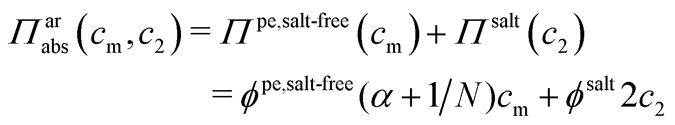
It has been shown experimentally that the “additivity rule” (ar) is a good approximation;38,52,53i.e., the contributions from the polyion with its counterions and those from the ion pairs of the salt in the cell can be regarded as independent and being the same as in a salt-free and polyelectrolyte-free solution (pure salt), respectively,
 | (10) |
As was done for the absolute ideal pressure with salt, the Donnan approach can be used to estimate the salt concentration in the cell for the additivity rule. It tends to underestimate the salt concentration and this becomes severe at higher polyelectrolyte concentrations, but then the salt concentration is low and the error matters less. However, the Donnan approach does not take non-ideality into account and another theory is needed to predict the osmotic pressure of the salt-free system, where the Poisson–Boltzmann cylinder with effective parameters might be a candidate, as indicated above.
4 Conclusions
We have performed both Monte Carlo simulations of single chains in a spherical cell model and molecular dynamics simulations of bulk systems with multiple chains with periodic boundary conditions to investigate the osmotic pressure of polyelectrolyte solutions. The coarse-grained description of the polyelectrolyte is in good agreement with experimental results of sodium polyacrylate.Although the single-chain cell-model simulations show a larger slope for the osmotic coefficient at high concentrations than the bulk simulations, especially for short chains, the qualitative features are the same.
An advantage of the cell model is that the pressure is calculated as the concentration of particles at the cell boundary, which allows a different perspective than the calculation through forces in the bulk simulations. In this view, it is clear that the counterions give the dominant contribution to the osmotic pressure. Moreover, the attractive electrostatic interactions between the polyion and its counterions reduce the counterion concentration at the boundary and gives an osmotic pressure that is lower than the ideal value.
For finite chains in a salt-free system, the osmotic pressure becomes ideal in the limit of infinite dilution. When the concentration is increased, the reduced volume allows the electrostatic polyion–counterion interactions to gain importance at the expense of the entropy that wants to spread the counterions evenly in the cell and the osmotic coefficient decreases.
At some point, however, the osmotic coefficient starts to increase. This non-monotonic behaviour has previously been attributed to the onset of a semi-dilute regime, but, as expressed in scaling theory, this implies a change in polyion–polyion interactions and we see no evidence that they are significant at these concentrations.
More direct evidence that a transition between a dilute and a semi-dilute regime (due to the polyion being a flexible polymer) is not necessary for the non-monotonic behaviour is the fact that it is also displayed by the Poisson–Boltzmann approximation applied to a solid sphere in a spherical cell. A possible explanation would be that the excluded volume of the sphere would increase the ideal pressure by reducing the volume available to the ions and lead to an increased osmotic coefficient, but after correcting for the change in ideal pressure, the Poisson–Boltzmann sphere still shows a non-monotonic behaviour. A similar correction for the chain simulations leads to the same conclusion.
In other words, we argue that the non-monotonic osmotic coefficient can be described as a consequence of the balance between only electrostatic interactions and entropy with the decreasing osmotic coefficient (as the concentration increases) at low concentrations being a finite-size effect and the increasing osmotic coefficient at high concentrations being a double-layer effect (the diffuse part of the double layer resists compression).
At a given monomer concentration, the osmotic coefficient is reduced, if either the charge density of the polyion or the chain length is increased, but a long-chain limit is reached, in the regime where the osmotic coefficient increases with concentration, already for chains with, in our case, about 100–200 monomers. This is also seen experimentally.
Parameters that reflect the linear nature of the polyion, contour length for size, linear charge density for charge, and contour-length concentration (contour length of a chain divided by the volume per chain), allow chains with different numbers of monomers, bond lengths, and degrees of ionisation to be represented as equivalent chains at low concentrations, at least as long as the different equivalent representations are not too diverse. At high concentrations, local interactions become significant and the exact nature of the model becomes important.
In equilibrium with a salt solution, the difference in osmotic pressure, i.e., the net osmotic pressure, is small at low polyelectrolyte concentrations, because salt enters the polyelectrolyte solution and makes it similar to the salt solution; i.e., produces a similar absolute osmotic pressure. At high polyelectrolyte concentrations, salt is prevented to enter the polyelectrolyte solution and the absolute osmotic pressure is essentially that of a salt-free solution, whereas the net osmotic pressure becomes smaller the higher the salt concentration (because the absolute pressure of the reference salt solution increases and the difference becomes smaller). The results show that the empirical additivity rule, i.e., to calculate the contributions from polyelectrolyte and the salt separately (one in the absence of the other), is a good approximation, which justifies the study of the salt-free polyelectrolyte system.
Conflicts of interest
There are no conflicts of interest to declare.Acknowledgements
Computational resources were provided by the Swedish National Infrastructure for Computing (SNIC) through Lunarc, the Centre for Scientific and Technical Computing at Lund University. The cylindrical Poisson–Boltzmann results were obtained using the analytical solution of Lifson and Katchalsky49 and the programme PBCell written by Bengt Jönsson was used for the PB sphere. Martin Turesson helped setting up the GROMACS calculations. Thanks also go to Bo Jönsson and Joaquim Li for valuable discussions.References
- N. Ise and T. Okubo, J. Phys. Chem., 1967, 71, 1287–1290 CrossRef.
- M. Reddy and J. A. Marinsky, J. Phys. Chem., 1970, 74, 3884–3891 CrossRef.
- Z. Alexandrowicz, J. Polym. Sci., 1959, 40, 113–120 CrossRef.
- V. A. Parsegian, R. P. Rand, N. L. Fuller and D. C. Rau, Methods Enzymol., 1986, 127, 400–416 Search PubMed.
- I. Pochard, J.-P. Boisvert, A. Malgat and C. Daneault, Colloid Polym. Sci., 2001, 279, 850–857 CrossRef.
- D. Bratko, D. Dolar and V. Vlachy, Vestn. Slov. Kem. Drus., 1981, 28, 321–325 Search PubMed.
- V. Vlachy and D. Dolar, J. Chem. Phys., 1982, 76, 2010–2014 CrossRef.
- M. J. Stevens and K. Kremer, Phys. Rev. Lett., 1993, 71, 2228–2231 CrossRef PubMed.
- M. J. Stevens and K. Kremer, J. Chem. Phys., 1995, 103, 1669–1690 CrossRef.
- M. Deserno, C. Holm, J. Blaul, M. Ballauff and M. Rehahn, Eur. Phys. J. E: Soft Matter Biol. Phys., 2001, 5, 97–103 CrossRef.
- M. Deserno, A. Arnold and C. Holm, Macromolecules, 2003, 36, 249–259 CrossRef.
- K. Arh, C. Pohar and V. Vlachy, J. Phys. Chem. B, 2002, 106, 9967–9973 CrossRef.
- Q. Liao, A. V. Dobrynin and M. Rubinstein, Macromolecules, 2003, 36, 3399–3410 CrossRef.
- R. Chang and A. Yethiraj, Macromolecules, 2005, 38, 607–616 CrossRef.
- D. Antypov and C. Holm, Phys. Rev. Lett., 2006, 96, 088302 CrossRef PubMed.
- D. Antypov and C. Holm, Macromolecules, 2007, 40, 731–738 CrossRef.
- J.-M. Y. Carrillo and A. V. Dobrynin, Macromolecules, 2011, 44, 5798–5816 CrossRef.
- J.-M. Y. Carrillo and A. V. Dobrynin, Polymers, 2014, 6, 1897–1913 CrossRef.
- R. Chang, Y. Kim and A. Yethiraj, Macromolecules, 2015, 48, 7370–7377 CrossRef.
- T. Alfrey, Jr., P. W. Berg and H. Morawetz, J. Polym. Sci., 1951, 7, 543–547 CrossRef.
- R. M. Fuoss, A. Katchalsky and S. Lifson, Proc. Natl. Acad. Sci. U. S. A., 1951, 37, 579–589 CrossRef.
- R. A. Marcus, J. Chem. Phys., 1955, 23, 1057–1068 CrossRef.
- H. Wennerström, B. Jönsson and P. Linse, J. Chem. Phys., 1982, 76, 4665–4670 CrossRef.
- B. Hess, C. Kutzner, D. van der Spoel and E. Lindahl, J. Chem. Theory Comput., 2008, 4, 435–447 CrossRef PubMed.
- D. van der Spoel, E. Lindahl, B. Hess, G. Groenhof, A. E. Mark and H. J. C. Berendsen, J. Comput. Chem., 2005, 1701–1719 CrossRef PubMed.
- D. van der Spoel, E. Lindahl, B. Hess, E. van Buuren, E. Apol, P. J. Meulenhoff, D. P. Tieleman, A. L. T. M. Sijbers, K. A. Feenstra, R. van Drunen and H. J. C. Berendsen, Gromacs User Manual version 4.5.4, http://www.gromacs.org, 2010 Search PubMed.
- B. Jönsson and H. Wennerström, J. Colloid Interface Sci., 1981, 80, 482–496 CrossRef.
- N. A. Metropolis, A. W. Rosenbluth, M. N. Rosenbluth, A. Teller and E. Teller, J. Chem. Phys., 1953, 21, 1087–1097 CrossRef.
- M. Lal, Mol. Phys., 1969, 17, 57–64 CrossRef.
- N. Madras and A. D. Sokal, J. Stat. Phys., 1988, 50, 109–186 CrossRef.
- D. Frenkel and B. Smit, Understanding Molecular Simulation, Academic Press, San Diego, 1996 Search PubMed.
- D. Henderson, L. Blum and J. L. Lebowitz, J. Electroanal. Chem., 1979, 102, 315–319 CrossRef.
- B. Widom, J. Chem. Phys., 1963, 39, 2808–2812 CrossRef.
- B. Svensson and C. E. Woodward, Mol. Phys., 1988, 64, 247–259 CrossRef.
- C. Parneix, J. Persello, R. Schweins and B. Cabane, Langmuir, 2009, 25, 4692–4707 CrossRef PubMed.
- B. Zhang, D. Yu, H.-L. Liu and Y. Hu, Polymer, 2002, 43, 2975–2980 CrossRef.
- W. Kern, Z. Phys. Chem., Abt. A, 1939, 184, 197–204 Search PubMed.
- Z. Alexandrowicz, J. Polym. Sci., 1962, 56, 115–132 CrossRef.
- K. Asai, K. Takaya and N. Ise, J. Phys. Chem., 1969, 73, 4071–4076 CrossRef.
- Z. Alexandrowicz, J. Polym. Sci., 1959, 40, 91–106 CrossRef.
- R. Kakehashi, H. Yamazoe and H. Maeda, Colloid Polym. Sci., 1998, 276, 28–33 CrossRef.
- T. A. Orofino, Recl. Trav. Chim. Pays-Bas, 1959, 78, 434–439 CrossRef.
- A. Katchalsky, Z. Alexandrowicz and O. Kedem, in Polyelectrolyte Solutions, ed. B. E. Conway and R. G. Barradas, John Wiley & Sons, New York, 1966, pp. 295–346 Search PubMed.
- M. Ullner and C. E. Woodward, Macromolecules, 2000, 33, 7144–7156 CrossRef.
- B. Jönsson, J. Persello, J. Li and B. Cabane, Langmuir, 2011, 27, 6606–6614 CrossRef PubMed.
- T. Odijk, Macromolecules, 1979, 12, 688–693 CrossRef.
- P.-G. de Gennes, Scaling Concepts in Polymer Physics, Cornell University Press, Ithaca, NY, 1979 Search PubMed.
- A. V. Dobrynin, R. H. Colby and M. Rubinstein, Macromolecules, 1995, 28, 1859–1871 CrossRef.
- S. Lifson and A. Katchalsky, J. Polym. Sci., 1954, 13, 43–55 CrossRef.
- G. S. Manning, J. Chem. Phys., 1969, 51, 924–933 CrossRef.
- A. Deshkovski, S. Obukhov and M. Rubinstein, Phys. Rev. Lett., 2001, 86, 2341–2344 CrossRef PubMed.
- Z. Alexandrowicz, J. Polym. Sci., 1960, 43, 337–349 CrossRef.
- A. Katchalsky and Z. Alexandrowicz, J. Polym. Sci., Part A: Gen. Pap., 1963, 1, 2093–2099 CrossRef.
| This journal is © The Royal Society of Chemistry 2018 |