
 Open Access Article
 This Open Access Article is licensed under a
 Creative Commons Attribution 3.0 Unported Licence
Automated separation of immiscible liquids using an optically monitored porous capillary†
James H.
Bannock
 ab,
Tsz Yin (Martin)
Lui
a,
Simon T.
Turner
a and
John C.
deMello
*ab
ab,
Tsz Yin (Martin)
Lui
a,
Simon T.
Turner
a and
John C.
deMello
*ab
aDepartment of Chemistry, Imperial College London, Exhibition Road, London SW7 2AY, UK. E-mail: j.demello@imperial.ac.uk
bCentre for Organic Electronic Materials, Department of Chemistry, NTNU, N-7491 Trondheim, Norway. E-mail: john.demello@ntnu.no
First published on 16th May 2018
Abstract
We report an automated procedure for the inline separation of two immiscible liquids based on a porous polytetrafluoroethylene (PTFE) capillary and a small number of inexpensive electronic components. By monitoring the light transmitted through fluid streams at the two outlets of the separator and iteratively adjusting a needle-valve located at one outlet until smooth time-invariant signals are observed at both outlets, the separator is capable of establishing complete liquid/liquid separation within minutes. Using mixtures of water and toluene as a test system, near quantitative recovery of the two liquids was achieved over a wide range of flow conditions without detectable cross contamination at either outlet. In a twenty-four hour test run, departures from complete separation occurred just three times, and on each occasion complete separation was automatically restored within ninety seconds. Further tests on other liquid/liquid mixtures showed that the automated separator is capable of rapidly and reliably inducing the separation of aqueous–organic, aqueous–fluorous and organic–fluorous mixtures, making it a versatile tool for numerous applications in fluidic analysis, synthesis and purification.
Introduction
Co-injection of two immiscible liquids into a narrow channel causes one or both components to segment into a train of discrete droplets or slugs.1,2 The resulting two-phase fluid stream has many applications in analytical and synthetic chemistry. Segmentation of a solvent, for instance, increases the degree of spatial confinement, providing a more uniform environment in terms of temperature and composition, which can be beneficial for chemical analysis or synthesis.2,3 Identical or distinct analyses/reactions can be carried out in individual slugs/droplets, allowing for the rapid acquisition of robust statistical data4 or the exhaustive screening of multiple reaction conditions.5 Biphasic reactions can be induced at the liquid–liquid interface.6 And purification can be performed inline,7 exploiting differences in solubility to extract selected solutes from one liquid into the other.In many cases, it subsequently becomes necessary to separate the immiscible liquids, while keeping at least one of the liquids flowing in a stable and controlled manner. Key applications of liquid–liquid separation include: (i) multistep chemical processing, where an intermediate purification or quench is required prior to further downstream processing;8 (ii) inline analysis, where switching to continuous flow can greatly simplify detection by removing the need for sophisticated detectors synchronised to the segmented solvent flow;9 and (iii) physical removal of the unwanted phase (and any impurities contained therein) prior to collection of the product.10
In microscale systems, phase separation is most effectively achieved using wetting-based methods that exploit differences in the tendency of the two liquids to wet a surface or membrane. One approach is to use micro-engineered structures to induce phase separation and coerce the two liquids into following separate exit paths as a result of one liquid maximizing and the other minimizing its contact with an exposed surface.11–19 Another approach, exploited in some commercial systems, is to use porous, planar membranes that can be selectively permeated by one of the two phases.5,20–24 When such membranes are used in conjunction with additional componentry to balance the pressure either side of the membrane, separation can be achieved at relatively high flow rates of up to 10 mL min−1![[thin space (1/6-em)]](https://www.rsc.org/images/entities/char_2009.gif) 24 (please see ref. 9 and 25 for recent reviews of methods for separating immiscible liquids on the microscale).
24 (please see ref. 9 and 25 for recent reviews of methods for separating immiscible liquids on the microscale).
We recently reported an alternative method for inline separation of immiscible liquids using a commercially sourced porous polytetrafluoroethylene (PTFE) capillary.9,26 Injection of a two-phase flow into the porous capillary causes one phase to preferentially permeate the capillary wall, leaving a continuous stream of the other phase to pass out of the capillary outlet. Insertion at the capillary outlet of a narrow flow restriction of appropriately chosen length and diameter allows the back pressure to be tuned for different flow conditions and liquid–liquid combinations, including aqueous–organic, aqueous–fluorous and organic–fluorous mixtures.
In this paper we demonstrate how a porous capillary can form the basis of a fully automated system for liquid/liquid separation that operates by optically monitoring the fluid streams extracted at the two outlets and iteratively modifying the back pressure downstream of the capillary to establish and subsequently maintain complete separation. Although simple in design, the automated separator induces rapid and reliable separation of a broad range of immiscible liquids, and should prove effective for many applications in microscale synthesis and analysis.
Principle of operation
For convenience we refer to the two liquids in the incoming segmented flow as the solvent and the carrier, the carrier being the phase that preferentially wets the walls of the separator. The solvent is typically understood to contain the reagents, products or analytes of interest, with the carrier acting as an inert liquid whose sole purpose is to maintain the segmented flow. However, this is not always so, and in many cases—e.g. biphasic reactions or liquid–liquid extractions—both phases participate in the chemical procedure.The principle of a porous capillary based separator is straightforward. The two-phase fluid stream enters the inlet of the porous capillary. The carrier preferentially wets and subsequently permeates the porous wall, accumulating on the exterior until it is of sufficient weight to drip from the capillary into a collection vial. This process repeats, with new carrier liquid collecting on the exterior of the porous capillary until the next drip occurs, thereby allowing the carrier to be extracted continuously from the channel without any drop in separation efficiency. A continuous (single-phase) stream of solvent is left flowing through the porous capillary and emerges at the outlet. The outflowing solvent may then be transferred to a vial for collection or passed into the next stage of a multistep chemical process as required. By encasing the porous capillary in an outer jacket, the carrier may be coerced into a continuous stream, allowing it too to be subjected to further flow processing. In this way, continuous separated streams of the two phases may be obtained at the separator outlets, see Methods and Fig. 1a.
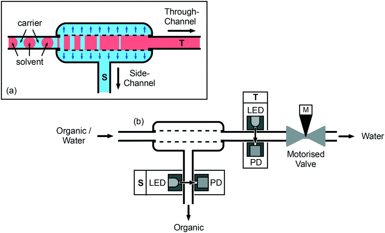 | ||
| Fig. 1 Principle of capillary-based liquid–liquid separation. (a) The segmented flow is passed into a short length of porous PTFE tubing, causing the carrier to preferentially wet and pass through the capillary wall into a jacket surrounding the capillary, where it is coerced into a continuous stream and extracted via a side-channel (S); the solvent passes through the porous capillary unaffected and emerges as a continuous stream via the through-channel (T); (b) automation is achieved by monitoring each outgoing fluid stream with a constant intensity light-emitting diode and a photodiode, and iteratively adjusting a motorized needle-valve at T until smooth non-fluctuating signals are obtained at both outlets (see scheme in Fig. 4). | ||
In the following discussion, we use the term through-channel (T) to describe the outlet at the end of the porous capillary, and the term side-channel (S) to describe the outlet connected to the wall of the porous capillary. To achieve complete separation of the two liquids, the back pressure at T must be carefully controlled: if it is too high, a fraction of the solvent will be forced through the capillary walls, leading to its incomplete recovery at T; if it is too low, a fraction of the carrier will pass through the entire length of the porous tubing without being depleted through the walls, causing a mixture of carrier and solvent to emerge at T. In previous work9,26 we achieved a suitable back pressure by inserting a narrow flow restriction of carefully selected length and diameter immediately after the through-channel outlet. For the work described here we use the same general approach of placing a flow restriction after T but, for ease of automation, the restriction takes the form of a needle-valve coupled to a stepper motor (M). Closing the valve via a clockwise turn of the stepper motor narrows the flow path and so increases the back pressure at T, making it easier for the liquids to pass through the porous capillary wall; opening the valve via an anticlockwise turn of the stepper motor has the opposite effect, making it easier for the liquids to pass straight through the capillary.
To automate the separation procedure, it is necessary to monitor the exiting fluid streams and iteratively modify the valve position until a single phase emerges at each outlet. The flow is monitored at each outlet using a light-emitting diode (LED) and a photodiode, located on opposing sides of the flow channel (see Fig. 1b). Each LED is driven by a constant current source to provide a near-constant light intensity. Hence, if the liquid/liquid separation is perfect and a single phase is flowing uniformly through each exit channel, the photodiodes at T and S will both generate stable, time-invariant photocurrents. On the other hand, if the separation is imperfect, at least one of the photodiodes will generate a fluctuating photocurrent due to scattering of incident light by the two-phase flow (scattering is caused by the different refractive indices of the two liquids, and so will occur even with colourless solutions). In-built transimpedance amplifiers within the casing of the photodiodes convert the photocurrents to voltages that are read at a rate of several hundred samples per second by a dual channel analogue to digital converter (ADC) coupled to a microcontroller. The microcontroller transfers the sampled data from the ADC to a personal computer (PC) for analysis and plotting, and periodically receives back from the PC an integer that specifies the number of steps through which the motor should move in the next iteration. The microcontroller in turn communicates with a stepper motor driver that delivers to the coils of the stepper motor the current waveforms required to execute the desired number of steps. For the needle-valve selected, just over one complete anticlockwise turn (equal to 400 full steps of the motor) is required to move the valve from fully closed to open. Full details regarding the construction and operation of the separator are provided in the Methods section.
Evaluation of separator in manual mode
The general behaviour of the separator was investigated using a segmented flow of water and toluene – a common solvent combination for liquid/liquid extractions.24 Toluene has a stronger affinity for PTFE than water and so, using the terminology introduced above, toluene is considered to be the carrier and water is considered to be the solvent. The segmented flow was generated by injecting the two liquids into the inlets of a two-input PTFE droplet generator (see Methods). The outlet of the droplet generator was in turn connected to the inlet of the separator by a short length of (non-porous) PTFE tubing, see Methods and Fig. 1b. The fluid streams from the two outlets of the separator were collected in separate vials.For initial testing, the flow rates of the solvent and carrier were set to equal values of 0.5 mL min−1. The valve was set to the fully closed position, and the system was allowed to stabilise for 90 s before acquiring data. Simultaneous thirty-second traces were then recorded for each channel (see bottom row of Fig. 2a). With the valve fully closed, the entire fluid stream was forced to pass through the walls of the porous capillary into the side channel, leading to a broadly static signal at T and a strongly fluctuating signal at S. The static nature of the T signal reflects the absence of liquid flow in the (closed) through-channel, while the irregular comb-like appearance of the S signal is characteristic of a disordered two-phase flow, in which alternating slugs of the two liquids are constantly crossing the detection zone.
 | ||
| Fig. 2 Variation of separator behaviour with valve position in the range 0 < V < 500. (a) Thirty-second traces recorded in the through-channel (red) and side-channel (blue) at valve positions in the range V = 0 (closed) to V = 500 (432°); traces were acquired 90 s after each change of valve position to allow time for the flow to stabilise; complete separation was attained at a valve position of V = 400, with smooth time-invariant signals being obtained in both channels. (b) Plot of T-channel RSD (red circles), S-channel RSD (blue circles) and differential RSD (black squares) versus valve position V, where the T-channel RSD is shown inverted for easier comparison with the differential RSD; RSD values were calculated using data from (a); a differential RSD value of −0.03% was obtained when the system was operating in a state of complete separation at V = 400. | ||
To determine the influence of the valve position V on the thirty-second traces, the valve was rotated anticlockwise – in fifty-step increments of the motor – from zero (closed) to five hundred (432°). Following each change of valve position, the system was allowed to stabilise for 90 s before recording the traces. For small rotations away from zero (V ≤ 350), the signals in the two channels resembled those seen for V = 0, with the side-channel signal fluctuating substantially and the through-channel signal remaining broadly static. At V = 400, the comb-like appearance of the S-channel went away, with both channels now exhibiting static signals, consistent with a single liquid phase being present in each channel. Inspection of the liquids collected at S and T revealed them to be toluene and water, respectively (as expected from the poorer wettability of water to PTFE). Hence, with the valve position set to V = 400, complete separation of the two liquids was achieved. Opening the valve further to V = 450 caused fluctuations to appear in T, indicating the valve had been opened too far and was now allowing some toluene to exit via the through-channel, alongside the water. Opening the valve still further, caused the majority of the injected two-phase stream to pass directly through the porous capillary into the T-channel.
The signal fluctuations in the S- and T-channels may be conveniently quantified in terms of the relative standard deviations, γS and γT. (Note, the relative standard deviation (RSD) γ of a signal is obtained by dividing its standard deviation σ by its mean μ: γ = σ/μ). Fig. 2b shows the variation of γS and γT with step position based on the transient data shown in Fig. 2a. To allow direct comparison with the parameter Δγ = γS − γT (introduced below), the RSD value of the T-channel is shown inverted in the diagram, i.e. we have plotted −γTversus valve position V. At V = 0, with the entire two-phase flow passing through the S-channel, the RSD was high in the S-channel (γS ≈ 14.1%) and low in the T-channel (γT ≈ 0.18%). The RSD values remained approximately constant until the valve position reached V = 350, at which point there was a slight reduction in the RSD value of the S-channel to 13.98%, followed by a much larger drop to 0.12% at V = 400. In the latter position complete separation of the two liquids was achieved, with the S- and T-channels both exhibiting low RSD values of 0.12% and 0.14%, respectively. Increasing V to 450 and beyond resulted in a substantial increase in the RSD value of the T-channel to 14.2% without substantially affecting the RSD value of the S-channel, consistent with a mixture of water and toluene passing through the T-channel and pure toluene passing through the S-channel.
To better understand the behaviour of the separator, a series of additional thirty-second traces was recorded in the vicinity of V = 400, using smaller ten-step increments (Fig. 3a). In moving from V = 350 to V = 370, lengthening periods of constant signal appeared in the S-channel trace, while the T-channel trace remained broadly static. This behaviour is consistent with a small amount of water – the liquid with poorer wettability to PTFE – passing into the T-channel (a reduction in the water content in the S-channel causes toluene to form longer slugs, leading to prolonged periods of constant signal in the S-channel trace). Inspection of the liquid extracted at T confirmed that it was indeed water, with no evidence of any contamination by toluene. Complete separation of the two liquids was achieved between V = 380 and V = 400, with both channels exhibiting static signals within this range. We refer to the range of valve positions that result in complete separation as the “separation window”. Increasing V to 410 caused occasional fluctuations to appear in the T-channel trace due to small amounts of toluene leaking into the through-channel as a result of insufficient back pressure at T. The T-channel fluctuations became more frequent as V was increased further from 420 to 450, consistent with a steadily rising toluene content in the through-channel. The RSD values extracted from the traces of Fig. 3a are shown in Fig. 3b. Inside the separation window 380 ≤ V ≤ 400, γS and γT had similar small values of <0.2%. To the left of the separation window (V < 380), γS rose rapidly to ∼14% while γT remained approximately constant at <0.2%. To the right of the separation window (V > 400), γT rose rapidly to ∼15% while γS remained approximately constant at <0.2%.
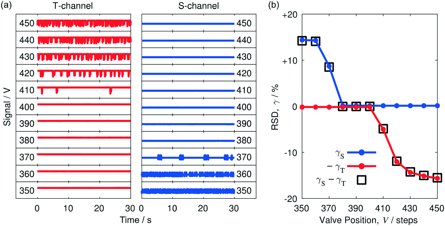 | ||
| Fig. 3 Variation of separator behaviour with valve position in the range 350 < V < 450. (a) Thirty-second traces recorded in the T-channel (red) and S-channel (blue) at valve positions in the range V = 350 (315°) to 450 (405°); traces were acquired 90 s after each change of valve position to allow time for the flow to stabilise; complete separation was attained for a narrow window of valve positions in the range 380 < V < 400, with smooth time-invariant signals being obtained in both channels. (b) Plot of T-channel RSD (red circles), S-channel RSD (blue circles) and differential RSD (black squares) versus valve position, where the T-channel RSD is shown inverted for easier comparison with the differential RSD; RSD values were calculated using data from (a); absolute differential RSD values of <0.01% were obtained in the separation window 380 < V < 400. | ||
Implementation of the automated separator
In the preceding section, we investigated the influence of the valve position on the steady-state signals in the two channels by manually stepping the valve position in fixed increments from zero, and then allowing the system to stabilise for a period of 90 s before recording each trace. In this way we identified a narrow window of valve positions within which complete separation of the two liquids could be achieved. The challenge in creating an automated system is to move the valve as rapidly as possible from its starting position to a position in the separation window, and thereafter to adjust the valve position as necessary to maintain complete separation. To ensure a fast response, it is necessary to avoid unnecessary delays by firstly keeping the time spent acquiring data in each iteration short and secondly moving the valve immediately after data acquisition. In other words, in each iteration it is necessary to update the valve position before the system has reached steady-state in the expectation that repeated adjustments of the valve position will quickly bring the system to a state of complete separation (despite individual measurements being made prematurely).From the discussion above, it is clear that the RSD values of the signals in the two channels provide useful diagnostic information about the instantaneous quality of the separation. Four scenarios can occur if the chosen solvent/carrier combination is separable: (i) the RSD may be high in the S-channel and low in the T-channel, indicating too much liquid is passing through the walls of the porous capillary and the valve should be loosened; (ii) the RSD may be low in the S-channel and high in the T-channel, indicating too much liquid is passing straight through the porous capillary and the valve should be tightened; (iii) the RSD may be low in both channels, indicating good separation; (iv) the RSD may be moderately high in both channels, indicating the valve position is close to the separation window but still requires some further tuning to achieve complete separation.
The direction of valve rotation needed to reach the separation window from a given starting position may be readily identified by subtracting the RSD value of the T-channel from the RSD value of the S-channel to obtain a differential RSD, Δγ = γS − γT. If Δγ is large and positive, too much liquid is passing through the walls of the porous capillary and the valve should be opened to reduce the back pressure at the end of the capillary; conversely, if Δγ is large and negative, too much liquid is passing straight through the porous capillary and the valve should be tightened. The variation of Δγ with valve position is indicated by the black squares in Fig. 2b and 3b. To the left of the separation window (V < 380) Δγ followed the behaviour of γS, while to the right of the separation window (V > 400), it followed the behaviour of −γT. Within the separation window |Δγ| was <0.1%.
High values of |Δγ| occur when the valve position is far from the separation window, meaning a large number of corrective steps are required to bring the system into a state of complete separation. Close to the separation window |Δγ| is smaller and fewer corrective steps are required. This suggests the use of a simple iterative algorithm, in which the number ΔV of corrective steps made within a single iteration scales linearly with the magnitude of Δγ from a value of zero when |Δγ| < Δγ0 to a maximum value of ΔV* when |Δγ| ≥ Δγ*, where Δγ0, Δγ* and ΔV* are user-defined tuning parameters for the optimisation routine. ΔV may be expressed as a piecewise function of Δγ:
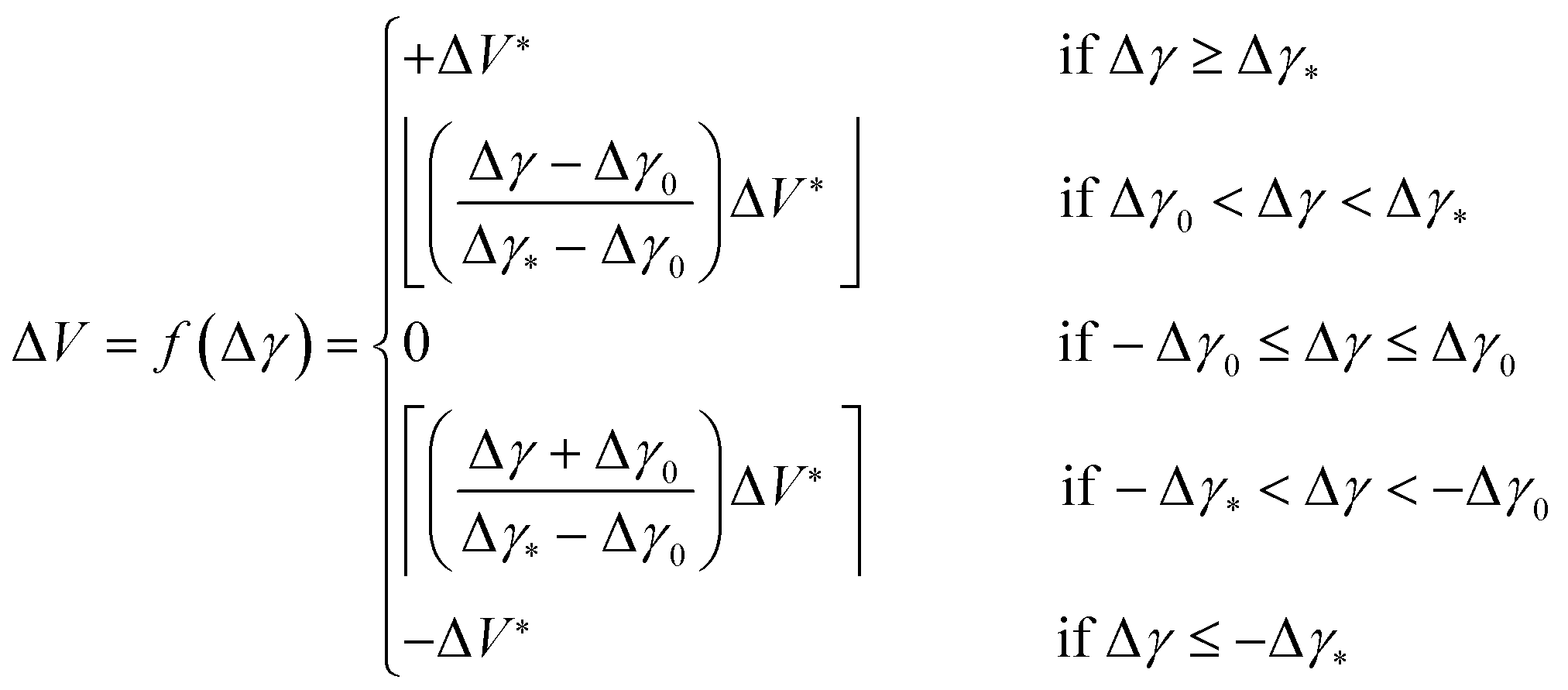 | (1) |
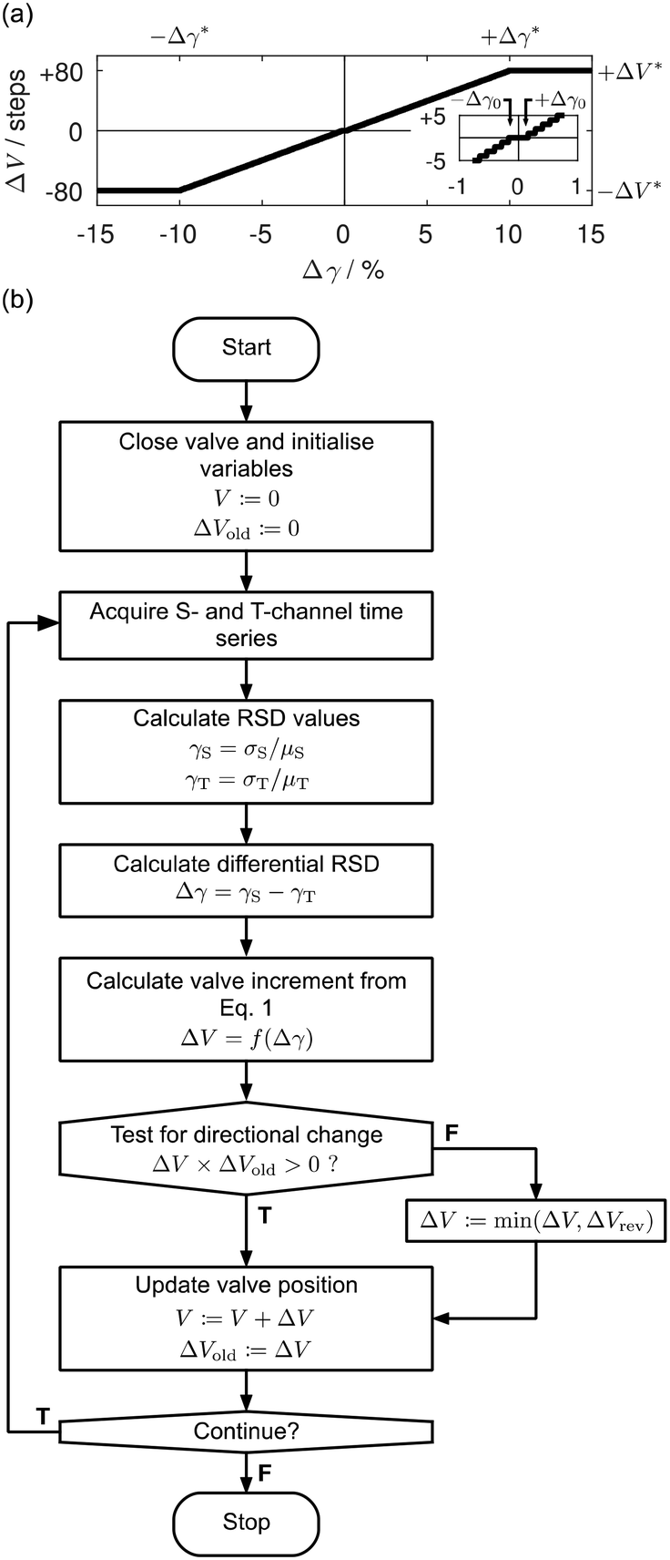 | ||
| Fig. 4 Details of optimisation procedure used to control the automated separator. (a) Graph showing the adjustment ΔV in the valve position versus the differential RSD Δγ, as defined by eqn (1); the valve adjustment, expressed in terms of discrete steps of the stepper motor, increases linearly from zero when |Δγ| = Δγ0 to ±ΔV* when |Δγ| = Δγ* and is always rounded to the nearest integer; it is set equal to zero for |Δγ| < Δγ0 and to ±ΔV* for |Δγ| > Δγ*; the inset graph shows ΔV versus Δγ for small values of Δγ. (b) Flow chart summarising the automated procedure used to bring the system into a state of complete separation: (i) the valve is closed and variables are initialized; (ii) five-second traces are recorded at the T- and S-channel outlets, and quantified in terms of their respective RSD values, γT and γS; (iii) the required adjustment ΔV of the valve position is determined from Δγ = γS − γT, using eqn (1); in the event ΔV is of opposite sign to the previous adjustment ΔVold then an upper limit of ΔV = ΔVrev is enforced; (iv) variables are updated and steps (ii) and (iii) are repeated until the end of the run. | ||
For the purposes of selecting Δγ0 and Δγ* it is useful to obtain approximate lower and upper limits on Δγ, which we denote Δγmin and Δγmax, respectively. Δγmin may be estimated by recording traces when the two channels are empty (i.e. when no liquid is present in the system, and any fluctuations in the signals are therefore entirely due to intrinsic noise in the detection system), while Δγmax may be estimated by blocking one of the exit channels and hence forcing the entire two-phase fluid stream through the other channel. Following this approach, we obtained values of 0.03% and ∼15% for Δγmin and Δγmax respectively.
The value of Δγ0 is chosen to avoid unnecessary movement of the valve when the system is operating in a state of complete separation, and so is typically set to be a small multiple of |Δγmin|. Δγ* is typically set to be slightly smaller than |Δγmax|, while ΔV* – the maximum permitted valve adjustment within a single iteration – is set empirically. Larger values of ΔV* ensure the separation window is approached more quickly, but excessively high values risk overshooting the separation window and may cause indefinite oscillation about the window (due to repeated overshooting), preventing convergence. In practice, a suitable value for ΔV* that is able to ensure rapid and reliable convergence may be easily determined by first setting the maximum angular rotation to a moderate value (e.g. 72°), and then increasing it if convergence is too slow or decreasing it if excessive overshooting occurs. In practice, once a satisfactory set of Δγ0, Δγ* and ΔV* values has been found for one particular liquid/liquid combination under a specific choice of flow condition, the same set of parameter values may be applied without adjustment to many other flow conditions and liquid/liquid combinations.
The optimisation routine continues to run even after complete separation has been achieved. Hence, in the event of an external disturbance that disrupts the separation, the optimisation routine will make whatever adjustments are needed from the current valve position V to restore the separation (there is no need to wind the valve back to the zero position and start again). The setting of a minimum threshold for |Δγ| – below which no corrective action is taken – is beneficial as it prevents the valve position from constantly “twitching” after a position in the separation window has been found, thereby avoiding needless perturbations to the pressure in the system. Only when a significant increase in |Δγ| occurs will the valve move to restore separation. Importantly, the optimisation procedure is robust against occasional anomalous signals (“blips”) in the measured signals due e.g. to gas bubbles passing through one of the detection zones: minor blips are ignored due to the minimum threshold for |Δγ|, while larger blips cause only a momentary adjustment to the valve position that is rapidly corrected once the anomaly has passed.
Preliminary testing of the algorithm in the form described above revealed that executing a large number of clockwise steps (ΔV ≪ 0) immediately after a series of anticlockwise steps (ΔV > 0) could cause a brief interruption of the flow in the side channel (until the pressure in the system had built up to the level needed to sustain flow), substantially increasing the time required to reach complete separation. To avoid this problem, for the first iteration only after a directional change, it was found necessary to cap the value of ΔV* at a small value ΔVrev (note, a change of direction may be readily detected by comparing the latest value of ΔV with its previous value ΔVold). The complete logic flow of the algorithm – including the correction for a change of direction – is summarised in Fig. 4b. All measurements reported below were obtained using the formulation described in the flow chart with the parameter values summarised in Table 1.
| Paramater | Value | Definition |
|---|---|---|
| S | 40 | Samples per second |
| Δt | 5 s | Duration of each trace |
| ΔV* | 80 steps | Maximum valve movement, equivalent to 72° |
| ΔVrev | 20 steps | Maximum valve movement after a directional change |
| Δγ0 | 0.1% | Minimum threshold for valve movement |
| Δγ* | 10% | Effective cap on Δγ. Values of Δγ ≥ Δγ* result in a valve movement of ΔV = ΔV* |
Evaluation of the automated separator
In Fig. 5 we show an optimisation run, obtained using a five-second data acquisition period and balanced injection rates of 0.5 mL min−1 each for toluene and water. The blue line in the lower plot indicates the variation of the valve position V with time, while the red line indicates the variation of the differential RSD Δγ with time. The red shaded zone spans differential RSD values in the range −Δγ* to +Δγ*, i.e. −10% to +10%. Δγ values lying outside the red zone result in the largest permitted adjustment of ±80 steps, while Δγ values lying inside the zone result in smaller adjustments that are proportional to the magnitude of Δγ. The adjustment ΔV to be made in the next iteration is shown in the upper plot, and can be seen to broadly follow the behaviour of Δγ due to the relationship described in eqn (1) and Fig. 4a. | ||
| Fig. 5 Behaviour of automated separator during initial convergence to complete separation. Plots showing valve adjustment ΔV (blue line, upper plot), valve position V (blue line, lower plot) and differential RSD value Δγ (red line, lower plot) versus time, using equal injection rates of 0.5 mL min−1 for water and toluene. Due to the mapping depicted in Fig. 4a, ΔV can be seen to have a similar profile to Δγ. Starting from an initial position of V = 0 in which the entire two-phase fluid stream was forced through S, a series of six large, positive Δγ values in excess of Δγ* were obtained at the start of the run, causing the valve to make six sequential positive adjustments at the maximum allowed adjustment of +80 steps. Δγ fell abruptly to <10−3% at the seventh iteration, causing the valve to hold its current position of V = 480; a series of large and negative Δγ values were then obtained, causing the valve to make five sequential negative adjustments. Owing to the change in direction, the first of these adjustments was capped at −20 steps (see main text). The remaining four steps occurred at the maximum permitted value of −80 steps, bringing the differential RSD to <10−1% at t = 1 min. Δγ remained at a similar low value for a further iteration, before turning positive. A series of four positive adjustments of the valve followed, bringing the system – on the nineteenth iteration (t = 1.5 min) – into a state of complete separation that persisted for the remainder of the ten-minute run (first two minutes shown only). | ||
Initially at V = 0, with the valve fully closed, the entire two-phase fluid stream was forced to pass through the side channel, leading to a high positive value of Δγ (17.3%) in excess of +Δγ* (10%). Consequently, the motor driving the valve made its maximum permitted adjustment of ΔV* = +80 steps. After the first valve adjustment, the differential RSD still exceeded +Δγ*, resulting in another adjustment of +80 steps. This behaviour continued until 0.5 min, at which point the differential RSD fell abruptly to an extremely small value of 10−3%, which lies far below the threshold Δγ0 (= 0.1%) for moving the valve. In the next iteration the valve therefore maintained its current position. Despite doing so, the next measured Δγ value was large and negative (−13.5%), indicating the optimiser had overshot the usable range and a two-phase fluid stream was now flowing in the through-channel. The significant change in Δγ despite the valve maintaining the same position is a consequence of the algorithm updating the valve position before the flow has stabilised.
Owing to the change in the sign of Δγ, the next valve adjustment occurred in the opposite (clockwise) direction and was consequently capped at a value of −ΔVrev = −20 steps. A series of −80 step adjustments followed until t = 1 min, when Δγ fell to a small value of ∼0.02%. Δγ remained at ∼0.02% for one further step – causing the motor to hold its current position – but then jumped to a value of 4.3%. During the next four iterations the valve advanced by +29, +80, +80 and +61 steps, finishing at a final position of V = 390 which was then maintained until the end of the optimisation run (t = 5 min). Δγ values during the last four iterations before convergence were +15.5, +13.6, +7.8 and −0.05% – the latter value falling below the threshold for a valve movement. The final valve position was reached just 1.5 min after beginning the optimisation run, with |Δγ| remaining below 0.02% for the remainder of the run and the system operating in a state of complete separation throughout this time.
To determine whether the separation was indeed complete – with pure toluene passing through the S-channel and pure water passing through the T-channel – the optimisation was repeated using a small amount of orange dye (Sudan) in the toluene and a small amount of blue dye (methylene blue) in the water. The system was allowed to converge, and samples of each liquid were then collected in separate vials over a ten minute period. Visual inspection of the collected solutions indicated complete separation of the two liquids, with no cross contamination evident in either channel, see inset photograph in Fig. 6. The optimisation was then repeated once again (without the dyes present), using mass balances to record – after convergence – the amount of liquid collected in each vial over a thirty minute period. The mass of liquid collected at each outlet increased linearly with time, indicating stable flow in both channels (see Fig. 6). By comparing the mass collection rate at each outlet to the mass injection rate from the corresponding syringe, the recovery rates were determined to be ∼99.5% and ∼98.5% for toluene and water, respectively (assuming fluid densities of 867 and 1000 g L−1). The slight shortfalls from 100% recovery are attributable to evaporative losses and/or systematic inaccuracies in the syringe specifications.
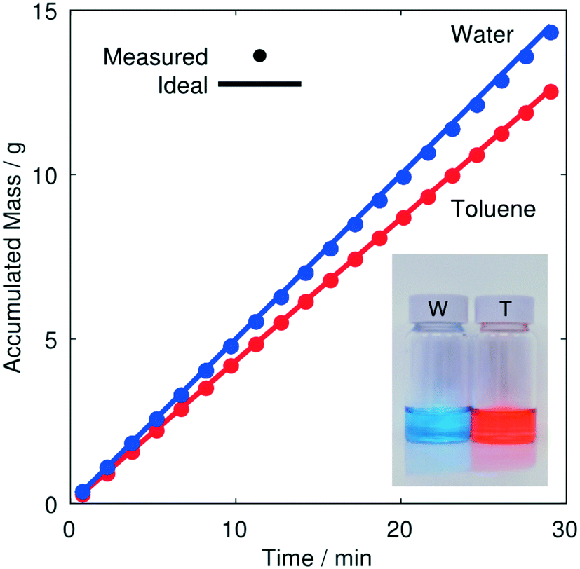 | ||
| Fig. 6 Throughput of automated separator. Graph showing masses of water and toluene collected at the T- and S-channel outlets versus time, using equal injection rates of 0.5 mL min−1. The masses were recorded after the separator had reached convergence. The circular markers denote experimental data, while the solid lines indicate ideal behavior, assuming perfect separation and 100% recovery of the two liquids. The close agreement between the experimental data and the ideal lines indicates near perfect separation, with the experimental data showing only marginal deviations from ideal behaviour due to slight evaporative losses or systematic inaccuracies in the syringe specifications. The inset shows a photograph of the liquids collected from the two outlets where, for ease of visualization, the water has been dyed blue and the toluene has been dyed orange. There is no evidence of cross-contamination in either channel, indicating complete separation of the two liquids. | ||
The ability of the separator to maintain complete separation over an extended period of time was investigated by carrying out a twenty-four hour run under the same flow conditions of 0.5 mL min−1 each for toluene and water. Following an initial 90 s convergence period, the two traces remained broadly static over the full duration of the run, with only three brief periods in which significant fluctuations appeared in the exit channel signals (see Fig. S1 and S2†) due to momentary departures from full separation or scattering of probe light by dust or air bubbles. In each case, the fluctuations lasted no more than ninety seconds, with the system then reverting to complete separation. Following the initial convergence period, 99.9% of the five-second traces recorded during the twenty-four-hour run had differential RSD values of 0.1% or below, corresponding to stable time-invariant signals in both channels, i.e. complete separation. Changes in the valve position were infrequent, with just thirteen adjustments being made during the course of the run, ranging in size from a single step to eighty steps, see Fig. S2.†
The performance of the automated separator under different flow conditions was determined by recording a series of optimisation runs at total flow rates in the range 0.2 to 10 mL min−1, using equal injection rates of water and toluene. The results are shown in Fig. 7a where, as before, blue lines indicate the variation of step position with time, while the red lines indicate the variation of the differential RSD with time. In all cases convergence was rapid, with complete separation being achieved in two and a half minutes or less. At the highest flow rates of 4 and 10 mL min−1, the system converged rapidly to complete separation in less than 1 min, with no overshoot of the separation window. Convergence also occurred within 1 min at 2 mL min−1, although there was a slight initial overshoot of the separation window that required subsequent correction. At slower flow rates ≤1 mL min−1 convergence to complete separation was less direct, with the step position adjusting repeatedly before complete separation was achieved. The complex convergence behaviour at low flow rates is a consequence of the physical design of the separator, which allows a small amount of water to become trapped in the side-channel jacket at the start of the run (when the complete fluid stream is passing through the S-channel). Later in the run, when fluid is flowing through both channels, the trapped water escapes intermittently into the side-channel outlet, resulting in anomalously high γS values that can cause the valve to make spurious movements in the positive direction, which must subsequently be corrected. Fortunately, owing to the low (<100 μL) dead volume of the jacket, the trapped water is soon depleted, causing the anomalous signals to cease. Hence convergence is still attained rapidly (<2.5 min), albeit by a complicated sequence of valve movements.
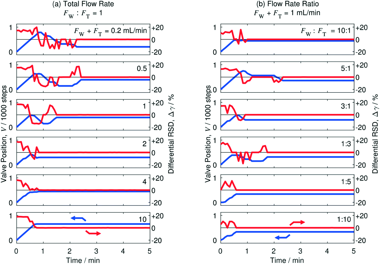 | ||
| Fig. 7 Performance of automated separator under various flow conditions. Each plot shows for a different flow condition the valve position V (blue line) and the differential RSD Δγ (red line) versus time, starting from an initial position of V = 0. The left plots (a) show the behaviour of the separator at various total flow rates F in the range 0.2 to 10 mL min−1, using equal injection rates of water and toluene. The right plots (b) show the behavior of the separator at various water-to-toluene flow rate ratios in the range 1:10 to 10:1, using a total flow rate of 1 mL min−1. In all cases, convergence to a state of complete separation was achieved in less than two and a half minutes, with complete separation then being maintained until the end of the five-minute run. | ||
The above results were obtained using equal flow rates for water and toluene, but the separator may also be applied in situations where the flow rates are imbalanced. In Fig. 7b, we show results for a series of runs using water-to-toluene flow-rate ratios in the range 1:10 to 10:1, keeping the total flow rate fixed at 1 mL min−1. Convergence was rapid in all cases, with complete separation again being achieved in two and a half minutes or less. Visual inspection of the collected solutions indicated complete separation of the two liquids in all cases, with no cross contamination evident in either channel, see Fig. S3.† Finally we note that, for maximum synthetic and analytic versatility, it is desirable that a separator should be able to handle a broad range of liquid/liquid combinations. In Fig. S4† we present additional data demonstrating the successful application of the separator to a number of commonly used organic/aqueous, fluorous/aqueous and fluorous/organic fluid streams, namely: dichloromethane/water, chloroform/water, hexane/water, cyclohexane/water, PFPE/water and PFPE/tetrahydrofuran, where PFPE denotes perfluorinated polyether. In all cases, complete separation of the two liquids was achieved with convergence times of a few minutes, confirming the broad applicability of the separator.
In summary we have described an autonomous inline liquid/liquid separator based on a porous PTFE capillary and a small number of inexpensive electronic components. By monitoring the light transmitted through fluid streams at the two outlets of the separator and iteratively adjusting a needle-valve located downstream of the porous capillary until smooth time-invariant signals are observed at both outlets, the separator is capable of establishing complete liquid/liquid separation within a few minutes. The simple construction of the separator, its ease of use, its low cost, and its good performance using a broad range of liquid combinations make it a promising tool for numerous applications in fluidic analysis, synthesis and purification.
Methods
Chemicals and raw materials
Chloroform, dichloromethane, hexane, tetrahydrofuran and toluene were purchased from VWR International. Cyclohexane was purchased from Sigma-Aldrich. Galden HT-170 perfluorinated polyether was purchased from Solvay Solexis. Aeos ePTFE microporous PTFE tubing (1.8 mm ID, 2.5 mm OD, 15–25 μm IND) was purchased from Zeus Industrial Products. PTFE tubing was purchased from IDEX Health & Science (3 mm ID, 4 mm OD), Polyflon Technologies (1 mm ID, 2 mm OD) and Kinesis (1 mm ID, 1/16′′ OD). Microfluidic connectors and adapters were purchased from IDEX Health & Science.Fabrication of the terminal blocks
The separator is housed within two terminal blocks that provide liquid-tight entry and exit ports for the microporous PTFE capillary and an exit pathway for liquid extracted through the porous membrane (the ‘side-channel’). Each terminal block (see Fig. S5†) was machined from a 25.5 mm by 25.5 mm by 12 mm block of PTFE. Flat-bottomed 1/4′′-28 and 5/16′′-24 threaded holes were machined coaxially into two opposing faces, A and A′, of the block to depths of 7.8 and 10 mm, respectively. A further 3 mm diameter hole was drilled centrally into the base of the threaded hole of face A′ to a depth of 4 mm. A channel running from A to A′ was then formed by drilling centrally from the base of the 1/4′′-28 threaded hole in face A to the opposing face, using a 2.5 mm bit. A second flat-bottomed 1/4′′-28 threaded hole was machined in the centre of the upper perpendicular face, B, to a depth of 7.8 mm, and a 2 mm hole was then drilled from its base to connect to the existing perpendicular channel.Assembly of the jacketed liquid–liquid separator
The separator was constructed from two identical PTFE ‘terminal blocks’ (I and II), a ∼120 mm length of porous capillary, an outer jacket formed from a 75 mm length of PTFE (3 mm ID, 4 mm OD), five flangeless ferrules, and six nuts. The two ends of the PTFE jacket were secured to the A′ faces of the two terminal blocks using ferrules and 5/16′′-24 nuts. Each end of the porous PTFE capillary was crimped to regular rigid PTFE tubing using a ferrule. The joined tubing was then secured in place, using a 1/4′′-28 nut in face A of each terminal block. The total length of exposed porous PTFE inside the jacket was 90.4 mm. The side channel outlet of the separator (face B of terminal block II) was connected to 2 mm PTFE tubing using a ferrule and 1/4′′-28 nut. The hole in face B of terminal block I was sealed off using a (closed) 1/4′′-28 nut. A photograph of an assembled jacketed separator is provided in Fig. S6.†Automated valve fabrication
The needle head of a micrometering needle valve (P-445, IDEX Health & Science) was joined coaxially to the shaft of a bipolar stepper motor (535-0401, RS Components), using a home-made spline coupling (see Fig. S7†). The stepper motor was driven using an Easydriver stepper motor controller (with microstepping disabled).Detector fabrication
Each optical detector was machined from a 35 mm by 21 mm by 15 mm block of black Delrin by first drilling a 2.1 mm-diameter connecting hole through the centres of two opposing faces (X and X′). A 1 mm cross-hole was then drilled through the middle of orthogonal faces of the block (Y and Y′), with the two holes meeting in the centre of the block. 1/4′′-28 screw threads were tapped around the holes in faces X and X′ to a depth of 7.5 mm, allowing them to accommodate flangeless ferrules and nuts of corresponding diameter. Mounting holes were then drilled in the middle of Y and Y′ to accommodate a bright-white LED (C503D-WAN, Cree) and an amplified photodiode (OPT101, Texas Instruments), respectively. 2 mm tubing from the appropriate outlet of the separator was threaded through X and X′, and secured in place using a ferrule and nut. Technical diagrams are shown in Fig. S8.† The LED was driven using a constant current source to achieve a stable light intensity. The voltage from the OPT101 was measured using an Adafruit ADS1115 16-bit analogue-to-digital converter (ADC) connected to an Arduino microcontroller, adjusting the gain of the ADS1115 to optimise the dynamic range of the ADC. The sample rate of the ADS1115 was set to 860 samples per second (430 samples per second per channel), with the Arduino applying a continuous ten-sample moving average to the data. The PC running the optimisation routine requested data from the Arduino at an approximate rate of 40 Hz.General flow configuration
All experiments except the extended twenty-four-hour run were carried out using a dual-channel syringe pump (Pump 33, Harvard Apparatus) to deliver the two fluid streams (carrier and solvent). For the twenty-four-hour run, a continuous delivery reciprocating syringe pump (Syrris, Asia) was used due to the higher liquid volumes needed. Aqueous and fluorous phases were delivered from 50 mL plastic syringes (HSW), and organic solvents were delivered from a 50 mL gas-tight glass syringe (SGE). For each combination of liquids, the two immiscible phases were connected to a two-input, one-output PTFE droplet-generator (see ref. 27 for a 3D design file) using standard microfluidic connectors and 1 mm ID, 1/16′′ OD PTFE tubing. The outlet of the droplet generator and the inlet of the separator were connected with a 250 mm length of 1 mm ID, 2 mm OD PTFE tubing. The through-channel of the separator was connected to the automated valve with a 100 mm length of 1 mm ID, 2 mm OD PTFE tubing (note, the choice of droplet generator was arbitrary, and the general performance of the separator is not noticeably affected by the nature of the two-phase flow or the manner of its generation).Data statement
Arduino and MATLAB code to operate the separator is available on Github: https://github.com/jdmgroup/Automated-Liquid-Liquid-Separator.Datasets generated during the current study and MATLAB plotting scripts are available in the Imperial College Box repository at: https://imperialcollegelondon.box.com/v/automated-liquid-separator.
Conflicts of interest
There are no conflicts to declare.Acknowledgements
This work was supported by an EPSRC Pathways to Impact Award (Impact Acceleration Account, Imperial College London) grant number EP/K503733/1. JHB was supported by an EPSRC Knowledge Transfer Secondment (Imperial College London) grant number EP/K503733/1 and an EPSRC Doctoral Prize Fellowship (Imperial College London). The authors thank Mr. Lee Tooley for fabricating the droplet generators.References
- S.-Y. Teh, R. Lin, L.-H. Hung and A. P. Lee, Lab Chip, 2008, 8, 198–220 RSC.
- D. Mark, S. Haeberle, G. Roth, F. von Stetten and R. Zengerle, Chem. Soc. Rev., 2010, 39, 1153 RSC.
- S. Mashaghi, A. Abbaspourrad, D. A. Weitz and A. M. van Oijen, TrAC, Trends Anal. Chem., 2016, 82, 118–125 CrossRef.
- Y. Zhu and Q. Fang, Anal. Chim. Acta, 2013, 787, 24–35 CrossRef PubMed.
- D. E. Angelescu, B. Mercier, D. Sless and R. Schroetter, Anal. Chem., 2010, 82, 2412–2420 CrossRef PubMed.
- M. J. Hutchings, B. Ahmed-Omer and T. Wirth, in Microreactors in Organic Chemistry and Catalysis, Wiley-VCH Verlag GmbH & Co. KGaA, Weinheim, Germany, 2013, pp. 197–219 Search PubMed.
- J. Britton and C. L. Raston, Chem. Soc. Rev., 2017, 46, 1250–1271 RSC.
- T. Noël, S. Kuhn, A. J. Musacchio, K. F. Jensen and S. L. Buchwald, Angew. Chem., Int. Ed., 2011, 50, 5943–5946 CrossRef PubMed.
- J. H. Bannock, T. W. Phillips, A. M. Nightingale and J. C. deMello, Anal. Methods, 2013, 5, 4991 RSC.
- A. M. Nightingale, J. H. Bannock, S. H. Krishnadasan, F. T. F. O'Mahony, S. A. Haque, J. Sloan, C. Drury, R. McIntyre and J. C. DeMello, J. Mater. Chem. A, 2013, 1, 4067–4076 Search PubMed.
- A. Günther, M. Jhunjhunwala, M. Thalmann, M. A. Schmidt and K. F. Jensen, Langmuir, 2005, 21, 1547–1555 CrossRef PubMed.
- E. Kolehmainen and I. Turunen, Chem. Eng. Process., 2007, 46, 834–839 CrossRef.
- M. N. Kashid, Y. M. Harshe and D. W. Agar, Ind. Eng. Chem. Res., 2007, 46, 8420–8430 CrossRef.
- O. K. Castell, C. J. Allender and D. A. Barrow, Lab Chip, 2009, 9, 388–396 RSC.
- F. Scheiff, M. Mendorf, D. Agar, N. Reis and M. Mackley, Lab Chip, 2011, 11, 1022–1029 RSC.
- W. A. Gaakeer, M. H. J. M. de Croon, J. van der Schaaf and J. C. Schouten, Chem. Eng. J., 2012, 207–208, 440–444 CrossRef.
- N. Assmann, S. Kaiser and P. Rudolf Von Rohr, J. Supercrit. Fluids, 2012, 67, 149–154 CrossRef.
- D. Liu, K. Wang, Y. Wang, Y. Wang and G. Luo, Chem. Eng. J., 2017, 325, 342–349 CrossRef.
- A. Ładosz and P. Rudolf von Rohr, Microfluid. Nanofluid., 2017, 21, 1–16 CrossRef.
- L. Nord and B. Karlberg, Anal. Chim. Acta, 1980, 118, 285–292 CrossRef.
- R. H. Atallah, J. Ruzicka and G. D. Christian, Anal. Chem., 1987, 59, 2909–2914 CrossRef.
- J. G. Kralj, H. R. Sahoo and K. F. Jensen, Lab Chip, 2007, 7, 256–263 RSC.
- A. E. Cervera-Padrell, S. T. Morthensen, D. J. Lewandowski, T. Skovby, S. Kiil and K. V. Gernaey, Org. Process Res. Dev., 2012, 16, 888–900 CrossRef.
- A. Adamo, P. L. Heider, N. Weeranoppanant and K. F. Jensen, Ind. Eng. Chem. Res., 2013, 52, 10802–10808 CrossRef.
- K. Wang and G. Luo, Chem. Eng. Sci., 2017, 169, 18–33 CrossRef.
- T. W. Phillips, J. H. Bannock and J. C. DeMello, Lab Chip, 2015, 15, 2960–2967 RSC.
- J. H. Bannock, S. H. Krishnadasan, M. Heeney and J. C. de Mello, Mater. Horiz., 2014, 1, 373–378 RSC.
Footnote |
| † Electronic supplementary information (ESI) available. See DOI: 10.1039/c8re00023a |
| This journal is © The Royal Society of Chemistry 2018 |