DOI:
10.1039/C8RA05956J
(Paper)
RSC Adv., 2018,
8, 35102-35130
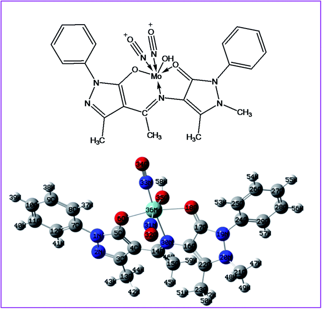
Nitric oxide functionalized molybdenum(0) pyrazolone Schiff base complexes: thermal and biochemical study†
Received
12th July 2018
, Accepted 28th September 2018
First published on 16th October 2018
Abstract
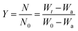
This work describes the synthesis and characterization of three molybdenum dinitrosyl Schiff base complexes of the general formula [Mo(NO)2(L)(OH)], where L is N-(dehydroacetic acid)-4-aminoantipyrene (dha-aapH), N-(4-acetylidene-3-methyl-1-phenyl-2-pyrazolin-5-one)-4-aminoantipyrine (amphp-aapH) or N-(3-methyl-1-phenyl-4-propionylidene-2-pyrazolin-5-one)-4-aminoantipyrine (mphpp-aapH). The complexes were formulated on the basis of spectroscopic analyses, elemental composition, magnetic susceptibility measurements, molar conductance behaviour and determination of the respective decomposition temperatures. A comparative experimental-theoretical approach was followed to elucidate the structure of the complexes. Fourier transform infra-red (FT-IR) spectroscopy, thermo-gravimetry (TG) and electronic spectral insights were mainly focused on the confirmation of the formation of the complexes. The computational density functional theory (DFT) calculations evaluated in the study involve the molecular specification for the use of LANL2DZ/RB3LYP formalism for metal atoms and 6-311G/RB3LYP for the remaining non-metal atoms. The study reveals a suitable cis-octahedral geometry for the complexes. The TG curve of one of the representative complexes was evaluated to find the respective thermodynamic and kinetic parameters using various physical methods. The Freeman & Carroll (FC) differential method, the Horowitz and Metzger (HM) approximation method, the Coats–Redfern method and the Broido method were employed to present a comparative thermal analysis of the complex. The Broido method proved the best fit to the results for the compound under question. In addition to structural and thermal analyses, the study also deals with the in vitro antimicrobial and anticancer sensitivity of the complexes. The results revealed potent biological properties of the representative complex containing dha-aapH. Cell toxicity tests against COLO-205 human cancer cell line using a 3-(4,5-dimethylthiazol-2-yl)-2,5-diphenyl-2H-tetrazolium bromide (MTT) assay showed an IC50 value of 53.13 μgm mL−1 for the Schiff base and 10.51 μgm L−1 for the respective complex. Similarly the same complex proved to be an effective antimicrobial agent against Aspergillus, Pseudomonas, E. coli and Streptococcus. The results indicated a more pronounced activity against Pseudomonas and Streptococcus than the other two microbial species.
Introduction
Molybdenum (Mo) is found in the active sites of enzymes such as nitrogenase, aldehyde oxidase, xanthine oxidase, sulfite oxidase, xanthine dehydrogenase and nitrate reductase. In attempts to find the antioxidant activity of various citrus fruit extracts molybdenum has been shown to have a special role.1 Molybdopterin has very recently been updated as one of the few molybdenum-containing compounds synthesized in nature. In animals, guanosine triphosphate (GTP) acts as a precursor.2,3 It has been found that the first two enzymes in the molybdopterin biosynthetic pathway, MoaA and MoaC, convert GTP into cyclic pyranopterin monophosphate (cPMP).4 The importance of molybdenum nitrosyl complexes, mimicking some biological phenomena has been updated recently.5 Similarly, analogues of this metal have been found to possess special role in catalysis.6–13 Nitric oxide tagged metal complexes of this class may serve as efficient tools to carry out apoptosis.14–16 Dinitrosylmolybdenum(0) complexes have also been reported to catalyze oligomerization and polymerization reactions of alkenes and alkynes and olefin metathesis.17–20 In particular, dinitrosyl complexes of iron have been proved to be biological intermediates formed during non-heme interaction with iron.21 Due to the biomimetic action of molybdenum in nitrite reduction it is assumed that a NO-labeled complex of molybdenum could act as an intermediate in the natural nitrogen fixation process.22 Recently NO assisted Mo-mediated catalysis has proven helpful in hydrodesulfurization.23
Nitric oxide expression in relation to hypertension, cancer and various other aspects has attracted chemists to tag the molecule with a framework for dwelling beneficial effects especially releasing and scavenging properties.24–33 In addition to experimental interests towards nitric oxide bound compounds, well fascinated investigations have been reportedly updated with respect to theoretical science of this class of compounds.34–37 There has been great ambiguity for the use of functionals and basis sets corresponding to such type of study. The use of various functionals and basis sets with respect to nitrosyl complexes to go through the chemical nature of NO as neutral or charged species has gained much importance in this regard.38–43
The selection of ligand for complexation is an important and careful job for synthesizing a complex. Pyrazolone based Schiff base as ONO donor ligand is the second co-ligand after NO targeted in this study. Such types of cyclic ligands have been found significant in various aspects.44–46 It has been revealed that pyrazole containing pharmacoactive agents play important role in medicinal chemistry.47 Pyrazolone derivatives are counted among typical ICT (Intramolecular Charge Transfer) compounds having well pronounced transport tendency.48–50 The derivatives of this class of compounds show fluorescence because of the double bond hindering, which occurs due to cyclization.51
In continuation of the interest towards synthetic chemistry and characterization based on various techniques, encompassing both theoretical and experimental approaches over metal nitrosyl complexes, a systematic study of the preparations and characterization of dinitrosyl complexes of Mo with the 4-aminoantipyrene based Schiff bases was aimed (Scheme 1). TG-base thermodynamic/kinetic and the biochemical study of these metallic systems are scarcely found. So in addition to formulation of the complexes, thermally evolved kinetic and thermodynamic parameters, in vitro antimicrobial and anticancer aspects are among the applied interests of the complexes reported herein.
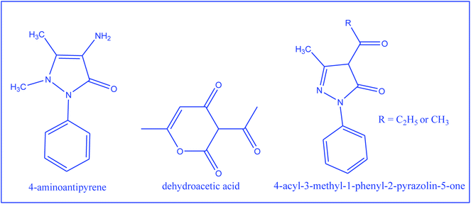 |
| | Scheme 1 2-D structure of compounds used for the synthesis of the Schiff bases. | |
Experimental section
Ammonium heptamolybdate tetrahydrate and dehydroacetic acid were products of Aldrich chemical Co., USA. 4-Aminoantipyrine was purchased from BDH Chemicals, Mumbai. 3-Methyl-1-phenyl-2-pyrozoline-5-one was supplied by Johnson Chemical Co., Bombay. Acetyl chloride and propionyl chloride were procured from Thomas Baker Chemicals Ltd, Mumbai. Hydroxylamine hydrochloride was acquired from Sisco Chem. Pvt. Ltd, Mumbai. All the chemicals were used as supplied without any further purification and were of AR Grade.
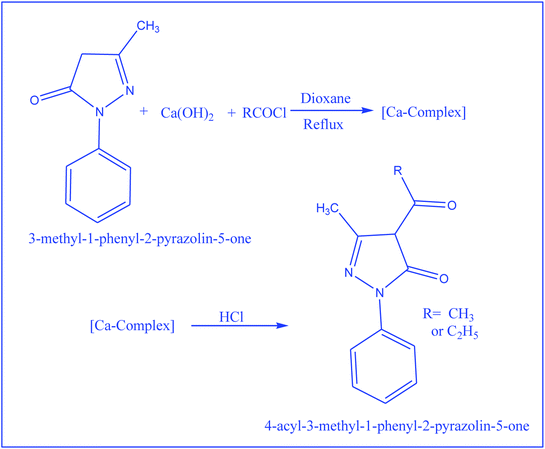
Synthesis of 4-acyl-3-methyl-1-phenyl-2-pyrazolin-5-one derivatives
4-Acyl-3-methyl-1-phenyl-2-pyrazolin-5-one derivatives were prepared by following the procedure reported earlier52 and were recrystallized from a methanol–water (9![[thin space (1/6-em)]](https://www.rsc.org/images/entities/char_2009.gif) :1) mixture. The reaction scheme related to the synthesis of 4-acyl-3-methyl-1-phenyl-2-pyrazolin-5-one is shown in Scheme 2.
:1) mixture. The reaction scheme related to the synthesis of 4-acyl-3-methyl-1-phenyl-2-pyrazolin-5-one is shown in Scheme 2.
 |
| | Scheme 2 Reaction scheme for the preparation of 2-pyrazoline derivatives. | |
Synthesis of Schiff bases
The Schiff base ligands were prepared by taking 1:1 ethanolic solution of dhaH (1.68 g, 10 mmol) or amphp (2.16 g, 10 mmol) or mphpp (2.30 g, 10 mmol) and 4-aminoantipyrine (2.03 g, 10 mmol) and refluxing the resulting solution for 5 h (Scheme 3). The reaction mixture was then poured into distilled water (250 mL), when a yellow precipitate was obtained. It was filtered, washed several times with water and then dried in vacuo. The physico-chemical analytical data of the Schiff base ligands are given in Table 1.
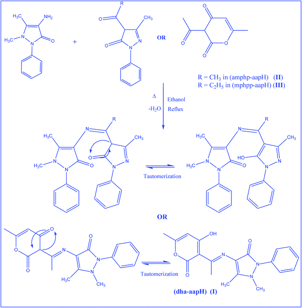 |
| | Scheme 3 Reaction schemes for the preparation of Schiff bases and associated keto–enol tautomerization. | |
Table 1 Physical and elemental analysis data of Schiff base ligands
| Compound (empirical formula) (F.W.) |
Analysis, found/(calc.) % |
Decom. temp. (°C) |
Yield (%) |
Colour |
| C |
H |
N |
| (dha-aapH) (I), C19H19N3O4) (353) |
64.00, (64.58) |
5.10, (5.42) |
11.30, (11.89) |
155 |
70 |
Light yellow |
| (amphp-aapH) (II), (C23H23N5O2) (401) |
68.50, (68.81) |
5.66, (5.77) |
17.30, (17.44) |
160 |
55 |
Light brown |
| (mphpp-aapH) (III), (C24H25N5O2) (415) |
69.20, (69.38) |
6.00, (6.06) |
16.66, (16.86) |
170 |
65 |
Golden yellow |
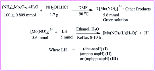
Synthesis of dinitrosylmolybdenum(0) complexes
All the complexes were prepared by following the method reported elsewhere.53 The reaction scheme demonstrating the synthesis of dinitrosyl complexes has been shown in Scheme 4. Their elemental analysis data, color, % yield, decomposition temperature and molar conductivities have been indicated in Table 2. All the complexes were tested for their solubility and were found partially soluble in ethanol and methanol, insoluble in water and soluble in DMSO and chloroform.
 |
| | Scheme 4 Schematic presentation of the synthesis of dinitrosylmolybdenum(0) complexes. | |
Table 2 Physical and elemental analysis data of molybdenumdinitrosyl complexes
| Compound (empirical formula) (F.W.) |
Analysis, found/(calc.) % |
Decom. temp. (C) |
Yield (%) |
Color |
Λm (Ω−1 cm2 mol−1) |
| C |
H |
N |
Mo |
| [Mo(NO)2(dha-aap)(OH)] (1), (C19H19MoN5O7) (525) |
43.00, (43.44) |
3.10, (3.65) |
12.90, (13.33) |
17.90, (18.27) |
195 |
70 |
Canary yellow |
26.4 |
| [Mo(NO)2(amphp-aap)(OH)] (2), (C23H23MoN7O5) (573) |
48.00, (48.17) |
3.98, (4.01) |
17.00, (17.10) |
16.20, (16.49) |
170 |
60 |
Golden yellow |
30.7 |
| [Mo(NO)2(mphpp-aap)(OH)] (3), (C24H25MoN7O5) (587) |
49.00, (49.07) |
4.13, (4.26) |
16.50, (16.70) |
16.20, (16.35) |
200 |
57 |
Middle buff |
25.3 |
Analytical techniques applied in the study
Carbon, hydrogen and nitrogen were determined micro analytically on Heraeus Carlo Erba 1108 elemental analyzer. The molybdenum content in each of the synthesized complexes was determined gravimetrically as MoO2(C9H6ON)2 by the method reported earlier.53 The identification of the coordinated nitrosyl group in the resulting complexes was made by the chemical method reported earlier.53
Magnetic measurements were performed by vibrating sample magnetometer method at RSIC, IIT Chennai. Electronic spectra of the complexes were recorded in dimethylformamide on an ATI Unicam UV-1-100 UV-Vis. Spectrometer in our laboratory. Conductance measurements were made at room temperatures in dimethylformamide using a Toshniwal conductivity bridge and dip-type cell with a smooth platinum electrode of cell constant 1.02. Decomposition temperatures of the Schiff bases and the chelates were recorded using an electrothermal apparatus having the capacity to record temperatures up to 360 °C. The IR spectra were recorded on a Perkin Elmer FTIR spectrophotometer using KBr pellets in our laboratory. Thermogravimetry curves of the complexes were recorded in the temperature range 50–1000 °C at the heating rate of 15 °C min−1 using a Mettler Toledo Stare System at the Regional Sophisticated Instrumentation Centre, Nagpur.
Biological assays
For testing the antimicrobial sensitivity, first a suitable medium was prepared by dissolving all components viz., yeast (2 gm), peptone (2 gm), dextrose (1 gm) and agar–agar (2 gm) in 100 mL distilled water and boiled to dissolve the medium completely. The medium was sterilized by autoclaving at 15 lbs pressure at 121 °C for 15 minutes. The autoclaved medium was mixed well and poured onto 100 mm Petriplates (25–30 mL per plate) while still molten. The antimicrobial screening was performed using agar-well diffusion method.54 Petriplates containing 20 mL Muller Hinton medium were seeded with 24 h culture of bacterial strains. Wells were cut and 20 μL of the given sample (of different concentrations) were added. The plates were then incubated at 37 °C for 24 hours. The antimicrobial activity was assayed by measuring the diameter of the inhibition zone formed around the well. Aspergillus, Pseudomonas, E. coli and Streptococcus were the cultures that were used. Ofloxacin as antibacterial and fluconazole as antifungal were the standard drugs used for comparing antimicrobial properties of the model molecular systems against the selected microbes.
Cell toxicity tests were investigated according to the method developed by Mosmann.55 COLO-205 human cancer Cell line was used for 3-(4,5-dimethylthiazol-2-yl)-2,5-diphenyl-2H-tetrazolium bromide (MTT) assay. Cells were plated in 96 well plates at 5000–7000 cell density per well. Cells were grown overnight in 100 μL of 10% FBS. After 24 hours cells were replenished with fresh media and the test samples were added to the cells. Different concentrations (10, 20, 40, & 80 mg L−1) of [dha-aapH] Schiff base and its [Mo(NO)2(dha-aap)OH] complex were added to wells in triplicates. Cells were incubated with the solution compounds for 24 hours at 37 °C in 5% CO2. After 24 hours 20 μL of MTT dye (5 mg mL−1) were added to each well and further incubated for 3 hours. Before read-out, precipitates formed were dissolved in 150 μL of DMSO using shaker for 15 minutes. All the steps performed after MTT additions were performed in dark. Absorbance was measured at 590 nm. Cell inhibition was determined by the following equation:
| % cell inhibition = 100 − {(At − Ab)/(Ac − Ab)} × 100 |
where,
At = absorbance value of test compound,
Ab = absorbance value of blank,
Ac = absorbance value of control.
Absorbance values that are lower than the control cells indicate a reduction in the rate of cell proliferation. Conversely, a higher absorbance rate indicates an increase in cell proliferation. Rarely, an increase in proliferation may be offset by cell death; evidence of cell death may be inferred from morphological changes.
| % cell survival = {(At − Ab)/(Ac − Ab)} × 100 |
| % cell inhibition = 100 − cell survival |
Computational methods
Density functional calculations were employed to investigate the vibrational properties and structural characteristics of the two representative compounds (amphp-aapH) (II) as ligand and the respective complex [Mo(NO)2(amphp-aap)(OH)] (2). The density functional theory (DFT) calculations with B3LYP/6-311+G specified for non-metallic content and B3LYP/LANL2DZ for Mo were used, respectively. The observed bands were assigned on the bases of results of normal coordinate analysis. All harmonic frequencies obtained were compared with real values to confirm each of the equilibrium geometries calculated corresponding to a minimum on the potential energy surface.56 Additionally, some of the calculated harmonic frequencies, particularly the NO stretch frequencies, were directly compared with the experimental frequencies. The assignment of the calculated wave numbers was aided by the animation option of Gauss View 5.0 graphical interface for Gaussian programs, which gives a visual presentation of the shape of the vibrational modes.57,58 The Cartesian representation of the theoretical force constants are usually computed at optimized geometry by assuming Cs point group symmetry. The energies of the highest occupied molecular orbital (HOMO) and lowest unoccupied molecular orbital (LUMO) levels were used for determining the existence of intramolecular charge transfer (ICT).59,100–106 UV-visible spectral calculation confined to TD-DFT approach were also separately computed for the two model systems.
Results and discussion
Comparative theoretical and experimental infrared spectral studies
The important infrared spectral bands of the Schiff base ligands and their complexes along with their tentative assignments are given in Tables 3 and 4, respectively. All the ligands used in the present investigation may exist in enol form as shown in Scheme 3. The ring nitrogen in these ligands is found to be inert towards coordination to molybdenum as revealed by no change in ν(C![[double bond, length as m-dash]](https://www.rsc.org/images/entities/char_e001.gif) N) (1583–1589 cm−1) of the free ligands after complexation. In fact, ν(CN) mode seems to be merged with ν(C–O) (cyclic) mode in the respective complexes. For a carbonyl donor, a significant shift of ν(CO) to lower wave number takes place because of the coordination through carbonyl oxygen. The ν(CO) for the cyclic carbonyl group at 1670, 1674 and 1669 cm−1 in uncoordinated dha-aapH, amphp-aapH and mphpp-aapH, respectively, is shifted to lower wave numbers and appears at 1575, 1581 and 1575 cm−1 in the respective complexes. This indicates that the cyclic carbonyl oxygen is bonded to molybdenum in these complexes.60 The FT-IR spectra of these ligands exhibit a strong band at 1632–1643 cm −1 assignable to ν(CN) (azomethine). In the spectra of the respective complexes this band is shifted to lower frequency, suggesting the coordination of the azomethine nitrogen to the metal centre.61 In all the complexes, the absence of a broad band centred at 3419–3440 cm−1 and the presence of a medium band at 1164–1186 cm−1 due to ν(C–O) (enolic) indicate the deprotonation and coordination of enolic oxygen to the metal centre.62 The appearance of two strong bands in the region 1773–1775 and 1645–1653 cm−1 and a weak band at 620–656 cm−1 may be assigned to ν(NO)+ and ν(Mo–NO), respectively, which are in agreement with previously reported results.63 The appearance of two ν(NO)+ bands in the spectra of all the synthesized complexes suggests the presence of a cis-[Mo(NO)2]2+ moiety in the complexes.64,65 The appearance of ν(OH) mode at 3410–3430 cm−1 in all the complexes under study is most probably due to presence of a coordinated hydroxyl group. The experimental FT-IR spectra of Schiff base ligands, I, II and III have been shown in Fig S1–S3.† The respective FT-IR spectra of the complexes 1, 2 and 3 are given in Fig S4–S6,† respectively.
N) (1583–1589 cm−1) of the free ligands after complexation. In fact, ν(CN) mode seems to be merged with ν(C–O) (cyclic) mode in the respective complexes. For a carbonyl donor, a significant shift of ν(CO) to lower wave number takes place because of the coordination through carbonyl oxygen. The ν(CO) for the cyclic carbonyl group at 1670, 1674 and 1669 cm−1 in uncoordinated dha-aapH, amphp-aapH and mphpp-aapH, respectively, is shifted to lower wave numbers and appears at 1575, 1581 and 1575 cm−1 in the respective complexes. This indicates that the cyclic carbonyl oxygen is bonded to molybdenum in these complexes.60 The FT-IR spectra of these ligands exhibit a strong band at 1632–1643 cm −1 assignable to ν(CN) (azomethine). In the spectra of the respective complexes this band is shifted to lower frequency, suggesting the coordination of the azomethine nitrogen to the metal centre.61 In all the complexes, the absence of a broad band centred at 3419–3440 cm−1 and the presence of a medium band at 1164–1186 cm−1 due to ν(C–O) (enolic) indicate the deprotonation and coordination of enolic oxygen to the metal centre.62 The appearance of two strong bands in the region 1773–1775 and 1645–1653 cm−1 and a weak band at 620–656 cm−1 may be assigned to ν(NO)+ and ν(Mo–NO), respectively, which are in agreement with previously reported results.63 The appearance of two ν(NO)+ bands in the spectra of all the synthesized complexes suggests the presence of a cis-[Mo(NO)2]2+ moiety in the complexes.64,65 The appearance of ν(OH) mode at 3410–3430 cm−1 in all the complexes under study is most probably due to presence of a coordinated hydroxyl group. The experimental FT-IR spectra of Schiff base ligands, I, II and III have been shown in Fig S1–S3.† The respective FT-IR spectra of the complexes 1, 2 and 3 are given in Fig S4–S6,† respectively.
Table 3 Important FT-IR spectral bands (cm−1) observed from of Schiff base ligands
| Schiff bases |
ν(CO) |
ν(CN) azomethine |
ν(CN) cyclic |
ν(OH) |
ν(C–OH) |
| I |
1670 |
1643 |
1583 |
3422 |
1155 |
| II |
1674 |
1625 |
1585 |
3419 |
1129 |
| III |
1669 |
1632 |
1589 |
3423 |
1162 |
Table 4 Important FT-IR spectral bands (cm−1) observed for molybdenumdinitrosyl complexes
| Complexes |
ν(NO)+ |
ν(CO) (ketonic) |
ν(CN) (azomethine) |
ν(C–O) (enolic) |
ν(HO) |
ν(Mo–NO) |
| 1 |
1773 |
1575 |
1598 |
1164 |
3428 |
621 |
| 1645 |
| 2 |
1775 |
1581 |
1604 |
1186 |
3410 |
656 |
| 1650 |
| 3 |
1774 |
1575 |
1602 |
1174 |
3413 |
620 |
| 1653 |
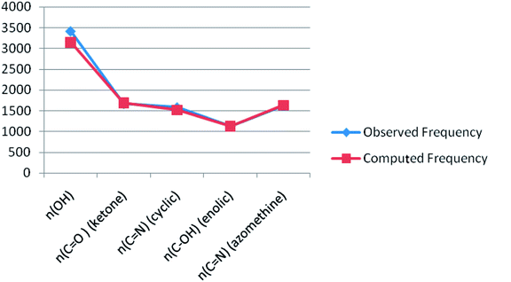
Theoretical FT-IR spectra of the representative ligand II and its complex are given in Fig. 1 and 2, respectively. DFT scheme for the calculation was same as described in geometrical optimization (vide supra) for both the compounds. The results are indicative of the absence of any imaginary frequency and hence stem the arrival of energy minimal surface for the optimized geometries. The main question of identification of functional groups solved by infra-red spectroscopy based on the computed and observed wave numbers are presented. Considering the composition of model compounds under study it is found that both the experimental spectra and spectra generated through Gaussian calculations are in close approx with one another. From the graphical interpretation, Fig. 3 and 4, it is noteworthy that the applied LANL2DZ/RB3LYP and RB3LYP/6-311G calculations fetch reliable frequency data. The main wave numbers (cm−1) computed for the ligand along with the particular assignments include ν(OH), 3154; ν(CO) (ketonic), 1691; ν(CN) (pyrazoline ring), 1513; ν(C–O) (enolic), 1123; ν(CN) (azomethine), 1636. The dinitrosyl complex is well characterized theoretically by highlighting the main frequency ranges entailed with the respective functional groups to mark the level of change that occurred to the ligand on complexation with the [Mo(NO)2]2+. The absence of ν(OH), 3154 and the existence of ν(OH, coordinated), 3738; ν(CO) (ketonic), 1596; ν(NO+), 1713, 1614; ν(CN) (azomethine), 1585; ν(C–O) (enolic), 1238; ν(Mo–NO+), 630. It is thus well established that the assumed cis geometry (C2v symmetry) with respect to the two NO ligands is comparable with theoretical outcomes. Other remarkable changes noticed on behalf of the ligand coordination are also obvious.
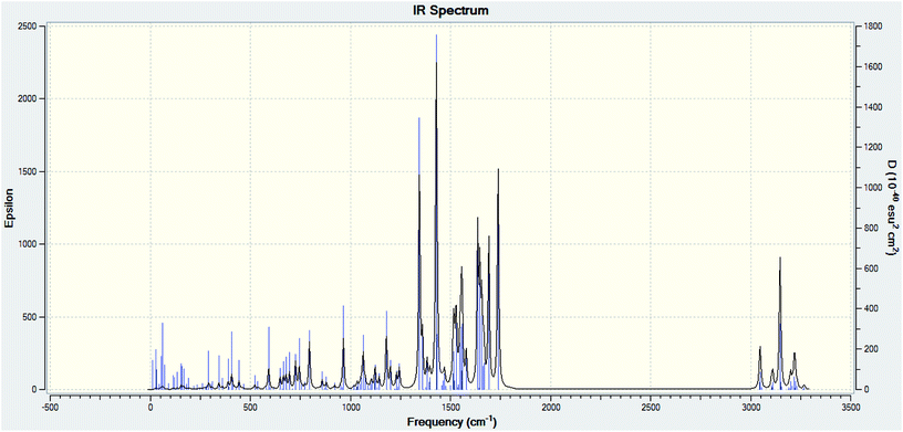 |
| | Fig. 1 Theoretical FT-IR spectrum of ligand II. | |
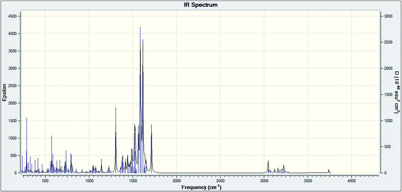 |
| | Fig. 2 Theoretical FT-IR spectrum of complex 2. | |
 |
| | Fig. 3 A plot of observed FT-IR frequency versus theoretical data of ligand II. | |
 |
| | Fig. 4 A plot of observed FT-IR frequency versus theoretical data of complex 2. | |
Experimental and theoretical electronic spectral studies
Experimental-electronic spectra of the complexes (Fig. S7–S9†) were recorded in 10−3 molar dimethyl DMF solutions. The electronic spectral peaks observed in each of the complexes along with their molar extinction coefficients are present in Table 5. All the complexes in the present investigation display five transitions. The assignments of these transitions have been given in the same table, and are based on molecular orbital diagram applicable to hexa coordinated dinitrosyl complexes reported elsewhere.66 These observations are in agreement with the results reported in the similar type of metallic systems.67 The presence of five excitation probabilities indicates the different types of bindings inside the system. The confirmation of this fashion can be directly co-related with the respective molecular orbital diagram designed for these type of metallic complexes given in Scheme 5.
Table 5 Electronic spectral data of complexes
| Complexes |
λmax |
ν (cm−1) |
(ε, litre cm−1 mol−1) |
Peak assignment |
| 1 |
274 |
36496 |
3722 |
1b2 → 2a2 |
| 296 |
33783 |
4312 |
1b2 → 3a1 |
| 325 |
30769 |
4582 |
1b2 → 2b2 |
| 349 |
28653 |
4821 |
1b2 → 1b1 |
| 440 |
22797 |
1942 |
1b2 → 2a1 |
| 2 |
293 |
34129 |
4110 |
1b2 → 2a2 |
| 329 |
30395 |
5255 |
1b2 → 3a1 |
| 356 |
28089 |
5046 |
1b2 → 2b2 |
| 387 |
25839 |
3021 |
1b2 → 1b1 |
| 444 |
22522 |
2722 |
1b2 → 2a1 |
| 3 |
289 |
33898 |
4411 |
1b2 → 2a2 |
| 313 |
31645 |
4666 |
1b2 → 3a1 |
| 339 |
28490 |
5141 |
1b2 → 2b2 |
| 357 |
27397 |
5054 |
1b2 → 1b1 |
| 416 |
21881 |
3480 |
1b2 → 2a1 |
 |
| | Scheme 5 Molecular orbital scheme for cis-dinitrosyl complexes of C2v symmetry. | |
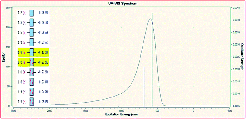
In order to explore the theoretical electronic spectral analysis, the TD-DFT LANL2DZ/RB3LYP and 6-311G/RB3LYP was applied for the representative ligand II and the complex 2. Pattern of electronic spectra of all the complexes carried out experimentally indicate the presence of an octahedral geometry around molybdenum that was correlated theoretically as well. DFT processed UV-visible spectra and simplified MO diagram (imposed over the spectra) for the ligand and complex are shown in Fig. 5 and 6, respectively. The particular alpha MO levels showing the possible transitions along with the energy required have been shown separately for the complex in Table 6. From the data obtainable from the log file of the respective complex confined to three possible excitations show the oscillator strengths f 0.005, 0.0021 and 0.0043 for λmax 1033.79 nm (1.1993 eV), λmax 683.87 nm (1.8130 eV) and λmax 574.47 nm (2.1582 eV), respectively. The non-zero oscillator strengths indicate that the values are acceptable to a considerable extent. Besides the above the excitation coefficients for the particular excitation have been used to calculate the percentage contribution of electronic transition for both the model compounds. From the data it is obvious that while 132 → 133 is the first preferred electronic transition, which are the respective HOMO → LUMO transitions of the dinitrosyl complex. Hence, the theoretical results indicate the relevance of the level of theory used for the electronic studies and an excellent NO-releasing capability is thus favoured.
 |
| | Fig. 5 TD-DFT UV-visible spectrum of ligand II with the overlayed MO levels. | |
 |
| | Fig. 6 TD-DFT UV-visible spectrum of complex 2 with overlayed MO levels. | |
Table 6 TD-DFT UV-visible data of [Mo(NO)2(amphp-aap)(OH)] (2) complex and the possible electronic transitions
| Excited state |
|
Excitation coefficient (C) |
Excitation contribution (%) |
| 1 |
Singlet A, 1.1993 eV, λmax = 1033.79 nm, f = 0.0005 |
| 130 → 133 |
0.21499 |
9.24 |
| 131 → 133 |
−0.26490 |
14.03 |
| 132 → 133 |
0.60770 |
73.86 |
| 2 |
Singlet A, 1.8130 eV, λmax = 683.87 nm, f = 0.0021 |
| 129 → 133 |
0.43924 |
38.59 |
| 130 → 133 |
0.22547 |
10.17 |
| 131 → 133 |
−0.42022 |
35.32 |
| 132 → 133 |
−0.25833 |
13.35 |
| 3 |
Singlet A, 2.1582 eV, λmax = 574.47 nm, f = 0.0043 |
| 129 → 133 |
0.49951 |
49.90 |
| 131 → 133 |
0.44629 |
39.83 |
| 132 → 133 |
0.18713 |
7.00 |
Molar conductance behaviour and magnetic susceptibility insights
The molar conductance measured in 10−3M DMF solutions of these complexes are in the range 25.3–45.4 Λ−1 cm2 mol−1 and thereby indicate the non-electrolytic nature of the complexes under investigation.68 The high molar conductance values are most probably due to strong donor capacity of dimethylformamide, which may lead to the displacement of anionic ligands and change of electrolyte type.68 The magnetic susceptibility measurements of these complexes indicate that they are diamagnetic and, hence, they should have ground states with a molecular orbital configuration (1a2)2 (1a1)2 and (1b2)2 following the molecular orbital diagram reported earlier.69 This result is consistent with the low-spin {Mo(NO)2}6 electron configuration of Mo(0) in these complexes. The diamagnetic and non electrolytic nature of these complexes also supports the presence of two NO+ groupings in all of these complexes.
Thermal analysis
Thermal methods of analysis are those techniques in which changes in physical and/or chemical properties of a substance are measured as a function of temperature. Methods that deal with changes in weight, dimensions or changes in energy come within this explanation. Thermogravimetry technique is entailed with the change in the weight of a substance recorded as a function of temperature or time, DTA (differential thermal analysis) in which the temperature difference between a substance and reference material as a function of temperature is recorded, DSC (differential scanning calorimetry) finds the application by giving a record of energy difference inputs into a substance and a reference material versus temperature function, EG (evolved gas analysis) where qualitative and quantitative evaluations of volatile products formed during thermal analysis are made and while as in TMA (thermo mechanical analysis) in which changes in dimensions of a substance are measured as a function of heat (temperature).70
The thermo-gravimetric analysis (TGA) for the representative dinitrosylmolybdenum(0) complex, 3 was carried out within the temperature range from ambient temperature to 1000 °C at the heating rate of 15 °C min−1. The first weight loss of 2.65% displayed by the compound at150 °C corresponds to the elimination of one hydroxyl group from the complex (calcd 2.89%). The compound exhibits some more weight losses, which we again could not correlate separately. However, the weight loss observed (83.5%) at 715 °C corresponds to the elimination of one hydroxo-, two nitrosyl-, and one ligand-group(s) from the complex (calcd 83.65%). The thermo-analytical curve of the compound is Fig. 7. Therefore, the TG-curve corroborates some of the assumptions made on the basis of infrared spectral studies for these complexes (vide supra).
 |
| | Fig. 7 Thermo-analytical curve of complex 3. | |
TG-based thermodynamics and kinetic studies
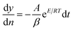
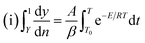
Thermal analysis is the means through which information concerning the thermal stability of the investigated complexes is obtained. In order to decide the number and stage of decomposition of water/hydroxyl or solvent molecules and whether they are inside or outside the coordination sphere TGA provides the ample information.71–73 The evaluation of kinetic and thermodynamic parameters involved in pyrolysis of compounds subjected to the investigation has gained keen interest based on choice of method out of various ways developed so far. In the present work Freeman and Carroll (FC) differential method, Horowitz and Metzger method, Coats and Redfern method and Broido method have been used to deal with the comparison studies of such methods to explore the thermodynamic and kinetic aspects of the concerned thermal behaviour of the representative complex.
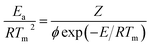
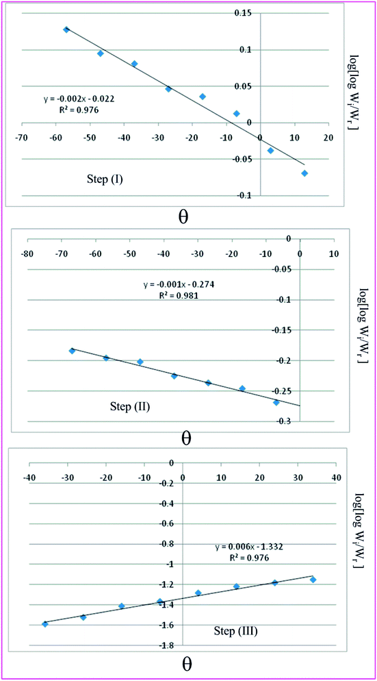
Freeman and Carroll, using Arrhenius equation gave the following equation:74
| |
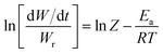 | (i) |
where
W is the total loss in weight up to time
t,
Wf is the weight loss at the completion of the reaction.
R is the gas constant and d
W/d
t is the weight time gradient,
Z is the pre-exponential factor and
Ea is the energy of activation.
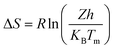
A plot of  against 1/T should be linear for decomposition following 1st order kinetics. The slope of plot gives the value of Ea, while the intercept is equal to lnZ, from which the pre exponential factor Z can be calculated. Having known the value of Z, the change in entropy ΔS can be calculated using equation
| |
 | (ii) |
where,
KB is the Boltzmann's constant,
h is Planck's constant and
Tm is the DTG peak temperature.
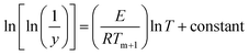
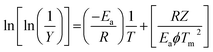
Horowitz and Metzger approximation involves the following expressions:75
| |
 | (v) |
where
W = mass loss at the completion of the reaction,
Wr =
W∞ −
W,
W is the mass loss at time ‘
t’,
Tm is the peak temperature,
R the gas constant,
θ =
T −
Tm and other terms same meaning as described earlier.
A plot of  against θ should gives a straight line with slope
  , from which from which Ea can be obtained. The frequency factor Z may be calculated using equation as
| |
 | (vi) |
where
ϕ is the constant heating rate, the thermodynamic parameters can be calculated as in previous case.
The Coats–Red fern equations are in the following form:76
| |
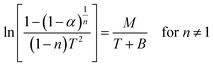 | (vii) |
| |
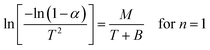 | (viii) |
where
α represents the fraction of sample decomposed at time
t, defined by
| |
 | (ix) |
W0,
Wt and
W∞ are the weight of sample before the degradation, at temperature
t °C and after total conversion respectively.
T is the derivative peak temperature
Ea,
R,
A and
ϕ are the heat of activation, the universal gas constant, pre-exponential factor and heating rate respectively.
The correlation coefficient ‘r’ was computed using the least square method for different values of n (n = 0.33, 0.5, 0.66 and 1), by plotting the LHS of eqn (iii) or (iv) versus T × 10−3
The n values which gave the best fit (n ≈ 1) were chosen as the order parameter for the decomposition stage of interest. From the intercept and linear slope of such stage, the A and Ea values were determined. ΔS was also computed using the relationship;
| |
 | (x) |
Δ
H and Δ
G are calculated using
eqn (ii) and
(iii); where
k is the Boltzmann's constant and
h is the Planck's constant.
Broido has developed a model and put forward a simple and sensitive graphical method for the treatment of TGA data.77 According to this method the weight at any time t (Wt) is related to the fraction of initial molecular weight as shown below
| |
 | (xi) |
where
W0 is the initial weight of the materials and
Wa is the weight of residue at the end of decomposition:
For isolated pyrolysis,
| |
 | (xii) |
and if
T is linear fraction of time
t, therefore:
| |
 | (xv) |
where,
β = d
T/
t, the heating rate.
Eqn (xv) is integrated as:
| |
 | (xvi) |
For the first order kinetics (n = 1) in which complex degrades usually:
| |
 | (xvii) |
On integrating and taking log of both sides of eqn (xvii), following equation is obtained.
| |
 | (xviii) |
Thus a plot of  vs. 1/T yields straight line, whose slope is directly related to Ea:
| | |
−Ea = slope × 2.303 × R
| (xix) |
where
Ea is the activation energy and
R is the gas constant. Application of this method is used to determine the kinetic parameter for the complexes.
| |
 | (xx) |
where,

and
Z can be calculated from the relation

The thermogram of the representative compound provided ample proof in all the methods reflecting the order of the decomposition of the order (n) of unity. The kinetic and thermodynamic parameters of the thermal degradation of the complexes namely, activation energy (Ea), enthalpy (ΔH), entropy (ΔS) and free energy changes (ΔG) were also calculated against the methods described above. The relevant parameters of each involved method at each step of decomposition were evaluated and are given Tables 7 and S1–S13.† The respective graphical presentations have also been given in Fig. 8–11. As all the methods employed in the study have certain advancements or limitations over one another. Hence, the different values and the comparative presentation confirm these assumptions. The summary of overall results can be explained as:
Table 7 Overall TGA evaluated thermodynamic parameters of (3)
| S. no. |
Methods |
Decomp. step |
Peak temp. (K) |
Ea (kJ mol−1) |
ΔH (kJ mol−1) |
ΔS (kJ mol−1) |
ΔG (kJ mol−1) |
lnZ (s−1) |
R2 |
| 1 |
Freeman Carroll |
1st |
530 |
24.543 |
20.136 |
−0.243 |
148.923 |
0.798 |
0.942 |
| 2nd |
710 |
18.781 |
12.878 |
−0.260 |
197.478 |
−0.9 |
0.804 |
| 3rd |
907 |
95.386 |
87.845 |
−0.020 |
105.475 |
11.4 |
0.966 |
| 2 |
Horowitz |
1st |
530 |
10.757 |
6.350 |
−0.242 |
134.610 |
0.955 |
0.976 |
| 2nd |
710 |
9.652 |
3.749 |
−0.248 |
179.829 |
0.473 |
0.981 |
| 3rd |
907 |
94.508 |
−102.049 |
−0.334 |
404.987 |
−9.66 |
0.976 |
| 3 |
Coats & Redfern |
1st |
530 |
−1.6196 |
−6.026 |
−0.230 |
115.875 |
2.322 |
0.967 |
| 2nd |
710 |
−0.472 |
−6.375 |
−0.231 |
157.635 |
2.582 |
0.900 |
| 3rd |
907 |
0.311 |
−7.230 |
0.232 |
203.194 |
2.611 |
0.957 |
| 4 |
Broido method |
1st |
530 |
0.078 |
−4.327 |
−0.104 |
50.793 |
17.521 |
0.982 |
| 2nd |
710 |
0.048 |
−5.855 |
−0.324 |
235.895 |
−8.652 |
0.961 |
| 3rd |
907 |
0.096 |
−7.440 |
−0.324 |
286.424 |
−8.455 |
0.982 |
| 5 |
Average |
1st |
530 |
8.440 |
4.033 |
−0.205 |
112.550 |
5.399 |
0.967 |
| 2nd |
710 |
7.002 |
1.100 |
−0.266 |
192.710 |
−1.624 |
0.911 |
| 3rd |
907 |
47.575 |
7.218 |
−0.227 |
250.02 |
−1.026 |
0.970 |
 |
| | Fig. 8 Freeman Carroll plots for the three thermal decomposition steps of complex 3. | |
 |
| | Fig. 9 Horowitz–Metzger plots for the three thermal decomposition steps of complex 3. | |
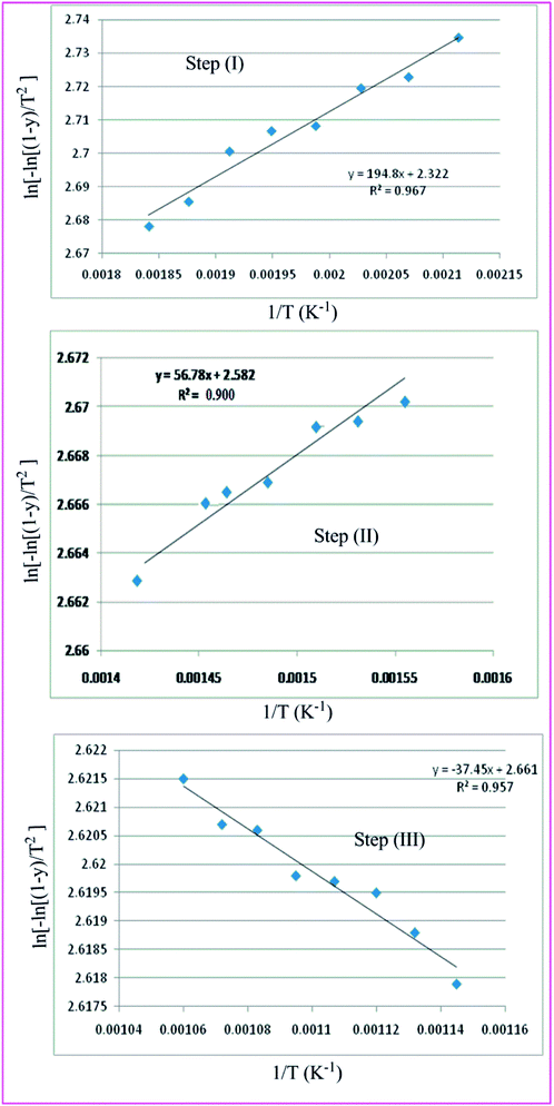 |
| | Fig. 10 Coats Redfern the three thermal decomposition steps of complex 3. | |
 |
| | Fig. 11 Broido the three thermal decomposition steps of complex 3. | |
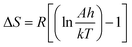
The value of change in entropy is an important factor describing the thermal stability of a coordination core. Low negative value of this factor is an indicative of more stable excited form as compared to the respective reactants of pyrolysis.78 In the later steps, numerical assignment shows increasing trend for the values of ΔG, although no regular trend is observed in the values of either Ea or ΔH. It is because of the fact that TΔS increases from one step to another, override in the values of ΔH is noticeable. Increasing values of ΔG for the subsequent steps of a given complex shows that the rate of mass loss will be lower than that of the precedent species.79,80 The structural rigidity of the remaining compound gets increased after the expulsion of one or more species, as compared with the precedent complex. From the values of ΔG we may confirm the coordination core where there attains increase in its value. It is known that the order has no intrinsic meaning, but is rather a mathematical smoothing parameter.81 In the present case the reaction order of all the decomposition stages of all the methods are found to nearly equal to one.
DFT based geometry optimization
The optimized geometry of both the model compounds furnished the zero point energy 280.99 kcal mol−1 for the representative complex, whereas 267.22 kcal mol−1 was the result obtained for the respective ligand. It directly reflects that the stability pronounces more in complex because of lower energy content. The various bond lengths, bond angles and dihedral angles generated from the equilibrium structure of one of the representative complex 2, using Gaussian 09 software are given in the Table 8. The computed bond lengths, such as, Mo(36)–O(6), Mo(36)–O(18), Mo(36)–O(35), Mo(36)–N(30), Mo(36)–N(31) and Mo(36)–N(33) in the present complex are 2.08248, 2.22730, 1.99819, 2.25960, 1.87183 and 1.82578 Å, respectively. The significant computed bond angles in the complex, such as, Mo(36)–O(35)–H(58), O(6)–Mo(36)–O(18), O(6)–Mo(36)–N(30), O(6)–Mo(36)–N(31), O(6)–Mo(36)–N(33), O(6)–Mo(36)–O(35), O(18)–Mo(36)–N(30), O(18)–Mo(36)–N(31), O(18)–Mo(36)–N(33), O(18)–Mo(36)–O(35), N(30)–Mo(36)–N(31), N(30)–Mo(36)–N(33), N(30)–Mo(36)–O(35), N(31)–Mo(36)–N(33), N(31)–Mo(36)–O(35), N(33)–Mo(36)–O(35) 123.52°, 165.10°, 86.98°, 95.96°, 98.15°, 88.80°, 78.50°, 87.88°, 96.19°, 85.17°, 90.97°, 174.23°, 79.65°, 91.09°, 169.27°, 97.76° respectively, suggest the octahedral structure of the present as well as the other complexes under investigation. The optimized structure of the representative complex is shown in Fig. 12. One of the interesting facts about the calculated bond angles is the prediction of linear nitrosyl group for the model complex by considering the bond angles like Mo(36)–N(33)–O(34), 176.807° and Mo(36)–N(31)–O(32), 172.092°.
Table 8 Optimized parameters of the representative complex 2
| S. no. |
Atom connectivity |
Bond length (angstrom) |
Atom connectivity |
Bond angle (°) |
Atom connectivity |
Dihedral angle (°) |
| 1 |
N(1)–N(2) |
1.4169 |
N(2)–N(1)–C(5) |
111.1227 |
C(5)–N(1)–N(2)–C(3) |
−0.6383 |
| 2 |
N(1)–C(5) |
1.3824 |
N(2)–N(1)–C(7) |
118.5364 |
C(7)–N(1)–N(2)–C(3) |
178.9895 |
| 3 |
N(1)–C(7) |
1.4305 |
C(5)–N(1)–C(7) |
130.3396 |
N(2)–N(1)–C(5)–C(4) |
−0.0469 |
| 4 |
N(2)–C(3) |
1.3357 |
N(1)–N(2)–C(3) |
106.2830 |
N(2)–N(1)–C(5)–O(6) |
178.3201 |
| 5 |
C(3)–C(4) |
1.4550 |
N(2)–C(3)–C(4) |
111.4977 |
C(7)–N(1)–C(5)–C(4) |
−179.6179 |
| 6 |
C(3)–C(13) |
1.5063 |
N(2)C–(3)–C(13) |
117.1144 |
C(7)–N(1)–C(5)–O(6) |
−1.2509 |
| 7 |
C(4)–C(5) |
1.4418 |
C(4)–C(3)–C(13) |
131.3541 |
N(2)–N(1)–C(7)–8(C) |
178.9105 |
| 8 |
C(4)–C(14) |
1.4302 |
C(3)–C(4)–C(5) |
104.3830 |
N(2)–N(1)–C(7)–C(12) |
−0.9442 |
| 9 |
C(5)–O(6) |
1.3079 |
C(3)–C(4)–C(14) |
129.3448 |
C(5)–N(1)–C(7)–C(8) |
−1.5450 |
| 10 |
O(6)–Mo(36) |
2.0825 |
C(5)–C(4)–C(14) |
126.2483 |
C(5)–N(1)–C(7)–C(12) |
178.6002 |
| 11 |
C(7)–C(8) |
1.4131 |
N(1)–C(5)–C(4) |
106.7018 |
N(1)–N(2)–C(3)–C(4) |
1.0728 |
| 12 |
C(7)–C(12) |
1.4132 |
N(1)–C(5)–O(6) |
122.5241 |
N(1)–N(2)–C(3)–C(13) |
179.1989 |
| 13 |
C(8)–C(9) |
1.4060 |
C(4)–C(5)–O(6) |
130.7492 |
N(2)-C(3)–C(4)–C(5) |
−1.0998 |
| 14 |
C(8)–H(37) |
1.0818 |
C(5)–O(6)–Mo(36) |
123.8363 |
N(2)–C(3)–C(4)–C(14) |
177.1843 |
| 15 |
C(9)C–(10) |
1.4070 |
N(1)–C(7)–C(8) |
121.4570 |
C(13)–C(3)–C(4)–C(5) |
−178.8776 |
| 16 |
C(9)–H(38) |
1.0875 |
N(1)–C(7)–C(12) |
118.4472 |
C(13)–C(3)–C(4)–C(14) |
−0.5936 |
| 17 |
C(10)–C(11) |
1.4089 |
C(8)–C(7)–C(12) |
120.0955 |
N(2)–C(3)–C(13)–H(42) |
−123.0107 |
| 18 |
C(10)–H(39) |
1.0872 |
C(7)–C(8)–C(9) |
119.3591 |
N(2)–C(3)–C(13)–H(43) |
−3.6297 |
| 19 |
C(11)–C(12) |
1.4037 |
C(7)–C(8)–H(37) |
119.8808 |
N(2)–C(3)–C(13)–H(44) |
115.5143 |
| 20 |
C(11)–H(40) |
1.0877 |
C(9)–C(8)–H(37) |
120.7601 |
C(4)–C(3)–C(13)–H(42) |
54.6664 |
| 21 |
C(12)–H(41) |
1.0829 |
C(8)–C(9)–C(10) |
120.9753 |
C(4)–C(3)–C(13)–H(43) |
174.0474 |
| 22 |
C(13)–H(42) |
1.0972 |
C(8)–C(9)–H(38) |
118.9494 |
C(4)–C(3)–C(13)–H(44) |
−66.8086 |
| 23 |
C(13)–H(43) |
1.0942 |
C(10)–C(9)–H(38) |
120.0753 |
C(3)–C(4)–C(5)–N(1) |
0.6517 |
| 24 |
C(13)–H(44) |
1.0972 |
C(9)–C(10)–C(11) |
119.1756 |
C(3)–C(4)–C(5)–O(6) |
−177.5308 |
| 25 |
C(14)–C(15) |
1.5222 |
C(9)–C(10)–H(39) |
120.4110 |
C(14)–C(4)–C(5)–N(1) |
−177.7028 |
| 26 |
C(14)–N(30) |
1.3441 |
C(11)–C(10)–H(39) |
120.4133 |
C(14)–C(4)–C(5)–O(6) |
4.1147 |
| 27 |
C(15)–H(45) |
1.0961 |
C(10)–C(11)–C(12) |
120.6755 |
C(3)–C(4)–C(14)–C(15) |
14.6302 |
| 28 |
C(15)–H(46) |
1.0927 |
C(10)–C(11)–H(40) |
120.0669 |
C(3)–C(4)–C(14)–N(30) |
−169.2415 |
| 29 |
C(15)–H(51) |
2.7989 |
(12)–C(11)–H(40) |
119.2576 |
C(5)–C(4)–C(14)–C(15) |
−167.431 |
| 30 |
C(15)–H(59) |
1.0919 |
C(7)–C(12)–C(11) |
119.7189 |
C(5)–C(4)–C(14)–N(30) |
8.6973 |
| 31 |
C(16)–C(17) |
1.4486 |
C(7)–C(12)–H(41) |
119.0313 |
N(1)–C(5)–O(6)–Mo(36) |
−169.9575 |
| 32 |
C(16)–C(22) |
1.3905 |
C(11)–C(12)–H(41) |
121.2498 |
C(4)–C(5)–O(6)–Mo(36) |
7.9777 |
| 33 |
C(16)–N(30) |
1.4094 |
C(3)–C(13)–H(42) |
112.0380 |
C(5)–O(6)–Mo(36)–O(18) |
−5.5974 |
| 34 |
C(17)–O(18) |
1.2861 |
C(3)–C(13)–H(43) |
108.2810 |
C(5)–O(6)–Mo(36)–N(30) |
−19.2260 |
| 35 |
C(17)–C(26) |
1.3807 |
C(3)–C(13)–H(44) |
112.1750 |
C(5)–O(6)–Mo(36)–N(31) |
−109.8906 |
| 36 |
O(18)–Mo(36) |
2.2273 |
H(42)–C(13)–H(43) |
108.3076 |
C(5)–O(6)–Mo(36)–N(33) |
158.1447 |
| 37 |
N(19)–N(20) |
1.4288 |
H(42)–C(13)–H(44) |
107.8519 |
C(5)–O(6)–Mo(36)–O(35) |
60.4738 |
| 38 |
N(19)–(24) |
1.4344 |
H(43)–C(13)–H(44) |
108.0491 |
N(1)–C(7)–C(8)–C(9) |
−179.9293 |
| 39 |
N(20)–C(21) |
1.4790 |
C(4)–C(14)–C(15) |
118.1067 |
N(1)–C(7)–C(8)–H(37) |
0.1013 |
| 40 |
N(20)–C(22) |
1.4083 |
C(4)–C(14)–N(30) |
121.0630 |
C(12)–C(7)–C(8)–C(9) |
−0.0769 |
| 41 |
C(21)–H(47) |
1.0909 |
C(15)–C(14)–N(30) |
120.7153 |
C(12)–C(7)–C(8)–H(37) |
179.9537 |
| 42 |
C(21)–H(48) |
1.0991 |
C(14)–C(15)–H(45) |
112.9048 |
N(1)–C(7)–C(12)–C(11) |
179.8937 |
| 43 |
C(21)–H(49) |
1.0925 |
C(14)–C(15)–H(46) |
108.8040 |
N(1)–C(7)–C(12)–H(41) |
−0.0733 |
| 44 |
C(22)–C(23) |
1.5003 |
C(14)–C(15)–H(51) |
83.6577 |
C(8)–C(7)–C(12)–C(11) |
0.0369 |
| 45 |
C(23)–H(50) |
1.0964 |
C(14)–C(15)–H(59) |
110.9281 |
C(8)–C(7)–C(12)–H(41) |
−179.9301 |
| 46 |
C(23)–H(51) |
1.0919 |
H(45)–C(15)–H(46) |
107.4605 |
C(7)–C(8)–C(9)–C(10) |
0.0714 |
| 47 |
C(23)–H(52) |
1.0983 |
H(45)–C(15)–H(51) |
56.0457 |
C(7)–C(8)–C(9)–H(38) |
−179.9715 |
| 48 |
C(24)–C(25) |
1.4085 |
H(46)–C(15)–H(51) |
163.0053 |
H(37)–C(8)–C(9)–C(10) |
−179.9595 |
| 49 |
C(24)–C(29) |
1.4101 |
H(46)–C(15)–H(59) |
107.9014 |
H(37)–C(8)–C(9)–H(38) |
−0.0025 |
| 50 |
C(25)–C(26) |
1.4055 |
H(51)–C(15)–H(59) |
76.8812 |
C(8)–C(9)–C(10)–C(11) |
−0.0251 |
| 51 |
C(25)–H(53) |
1.0845 |
C(17)–C(16)–C(22) |
107.0607 |
C(8)–C(9)–C(10)–H(39) |
179.9615 |
| 52 |
C(26)–C(27) |
1.4084 |
C(17)–C(16)–N(30) |
116.4175 |
H(38)–C(9)–C(10)–C(11) |
−179.9817 |
| 53 |
C(26)–H(54) |
1.0866 |
C(22)–C(16)–N(30) |
136.2783 |
H(38)–C(9)–C(10)–H(39) |
0.0050 |
| 54 |
C(27)–C(28) |
1.4087 |
C(16)–C(17)–O(18) |
125.9228 |
C(9)–C(10)–C(11)–C(12) |
−0.0160 |
| 55 |
C(27)–H(55) |
1.0867 |
C(16)–C(17)–N(19) |
107.7631 |
C(9)–C(10)–C(11)–H(40) |
−180.0051 |
| 56 |
C(28)–C(29) |
1.4054 |
O(18)–C(17)–N(19) |
126.2938 |
H(39)–C(10)–C(11)–C(12) |
179.9973 |
| 57 |
C(28)–H(56) |
1.0869 |
C(17)–O(18)–Mo(36) |
108.5794 |
H(39)–C(10)–C(11)–H(40) |
0.0083 |
| 58 |
C(29)–H(57) |
1.0867 |
C(17)–N(19)–N(20) |
108.6248 |
C(10)–C(11)–C(12)–C(7) |
0.0099 |
| 59 |
N(30)–Mo(36) |
2.2596 |
C(17)–N(19)–C(24) |
127.2127 |
C(10)–C(11)–C(12)–H(41) |
179.9762 |
| 60 |
N(31)–O(32) |
1.2258 |
N(20)–N(19)–C(24) |
122.6405 |
H(40)–C(11)–C(12)–C(7) |
179.9991 |
| 61 |
N(31)–Mo(36) |
1.8718 |
N(19)–N(20)–C(21) |
116.7843 |
H(40)–C(11)–C(12)–H(41) |
−0.0347 |
| 62 |
N(33)–O(34) |
1.2199 |
N(19)–N(20)–C(22) |
107.0216 |
C(4)–C(14)–C(15)–H(45) |
−75.6720 |
| 63 |
N(33)–Mo(36) |
1.8258 |
C(21)–N(20)–C(22) |
122.5219 |
C(4)–C(14)–C(15)–H(46) |
43.5349 |
| 64 |
O(35)–Mo(36) |
1.9982 |
N(20)–C(21)–H(47) |
109.4412 |
C(4)–C(14)–C(15)–H(51) |
−124.5978 |
| 65 |
O(35)–H(58) |
0.9770 |
N(20)–C(21)–H(48) |
111.7617 |
C(4)–C(14)–C(15)–H(59) |
162.0808 |
| 66 |
|
|
N(20)–C(21)–H(49) |
108.5134 |
N(30)–C(14)–C(15)–H(45) |
108.1856 |
| 67 |
|
|
H(47)–C(21)–H(48) |
109.0236 |
N(30)–C(14)–C(15)–H(46) |
−132.6075 |
| 68 |
|
|
H(47)–C(21)–H(49) |
108.2197 |
N(30)–C(14)–C(15)–H(51) |
59.2598 |
| 69 |
|
|
H(48)–C(21)–H(49) |
109.8128 |
N(30)–C(14)–C(15)–H(59) |
−14.0616 |
| 70 |
|
|
C(16)–C(22)–N(20) |
109.0522 |
C(4)–C(14)–N(30)–C(16) |
174.9123 |
| 71 |
|
|
C(16)–C(22)–C(23) |
130.3368 |
C(4)–C(14)–N(30)–Mo(36) |
−29.3835 |
| 72 |
|
|
N(20)–C(22)–C(23) |
120.4189 |
C(15)–C(14)–N(30)–C(16) |
−9.0602 |
| 73 |
|
|
C(22)–C(23)–H(50) |
111.3545 |
C(15)–C(14)–N(30)–Mo(36) |
146.644 |
| 74 |
|
|
C(22)–C(23)–H(51) |
109.6027 |
C(14)–C(15)–H(51)–C(23) |
−114.8123 |
| 75 |
|
|
C(22)–C(23)–H(52) |
112.3257 |
H(45)–C(15)–H(51)–C(23) |
122.0302 |
| 76 |
|
|
H(50)–C(23)–H(51) |
107.3773 |
H(46)–C(15)–H(51)–C(23) |
106.9489 |
| 77 |
|
|
H(50)–C(23)–H(52) |
107.8412 |
H(59)–C(15)–H(51)–C(23) |
−1.5508 |
| 78 |
|
|
H(51)–C(23)–H(52) |
108.1619 |
C(22)–C(16)–C(17)–O(18) |
−173.3069 |
| 79 |
|
|
N(19)–C(24)–C(25) |
118.8474 |
C(22)–C(16)–C(17)–N(19) |
5.1364 |
| 80 |
|
|
N(19)–C(24)–C(29) |
120.2177 |
N(30)–C(16)–C(17)–O(18) |
1.9510 |
| 81 |
|
|
C(25)–C(24)–C(29) |
120.9133 |
N(30)–C(16)–C(17)–N(19) |
−179.6057 |
| 82 |
|
|
C(24)–C(25)–C(26) |
119.1193 |
C(17)–C(16)–C(22)–N(20) |
−7.1042 |
| 83 |
|
|
C(24)–C(25)–H(53) |
119.9464 |
C(17)–C(16)–C(22)–C(23) |
167.7644 |
| 84 |
|
|
C(26)–C(25)–H(53) |
120.9216 |
N(30)–C(16)–C(22)–N(20) |
179.0453 |
| 85 |
|
|
C(25)–C(26), (27) |
120.5469 |
N(30)–C(16)–C(22)–C(23) |
−6.0861 |
| 86 |
|
|
C(25)–C(26)–H(54) |
119.3406 |
C(17)–C(16)–N(30)–C(14) |
145.8735 |
| 87 |
|
|
C(27)–C(26)–H(54) |
120.1122 |
C(17)–C(16)–N(30)–Mo(36) |
−12.9098 |
| 88 |
|
|
C(26)–C(27)–C(28) |
119.7778 |
C(22)–C(16)–N(30)–C(14) |
−40.6926 |
| 89 |
|
|
C(26)–C(27)–H(55) |
120.1215 |
C(22)–C(16)–N(30)–Mo(36) |
160.5240 |
| 90 |
|
|
C(28)–C(27)–H(55) |
120.0984 |
C(16)–C(17)–O(18)–Mo(36) |
10.4761 |
| 91 |
|
|
C(27)–C(28)–C(29) |
120.2899 |
N(19)–C(17)–O(18)–Mo(36) |
−167.6845 |
| 92 |
|
|
C(27)–C(28)–H(56) |
120.1302 |
C(16)–C(17)–N(19)–N(20) |
−1.2310 |
| 93 |
|
|
C(29)-C(28)–H(56) |
119.5706 |
C(16)–C(17)–N(19)–C(24) |
164.8452 |
| 94 |
|
|
C(24)–C(29)–C(28) |
119.3367 |
O(18)–C(17)–N(19)–N(20) |
177.2049 |
| 95 |
|
|
C(24)–C(29)–H(57) |
119.9739 |
O(18)–C(17)–N(19)–C(24) |
−16.7189 |
| 96 |
|
|
C(28)–C(29)–H(57) |
120.6705 |
C(17)–O(18)–Mo(36)–O(6) |
−26.4786 |
| 97 |
|
|
C(14)–N(30)–C(16) |
125.0868 |
C(17)–O(18)–Mo(36)–N(30) |
−12.5851 |
| 98 |
|
|
C(14)–N(30)–Mo(36) |
123.2236 |
C(17)–O(18)–Mo(36)–N(31) |
78.8398 |
| 99 |
|
|
C(16)–N(30)–Mo(36) |
107.9961 |
C(17)–O(18)–Mo(36)–N(33) |
169.7075 |
| 100 |
|
|
Mo(36)–O(35)–H(58) |
123.5183 |
C(17)–O(18)–Mo(36)–O(35) |
−92.9858 |
| 101 |
|
|
O(6)–Mo(36)–O(18) |
165.0647 |
C(17)–N(19)–N(20)–C(21) |
−144.7408 |
| 102 |
|
|
O(6)–Mo(36)–N(30) |
86.9854 |
C(17)–N(19)–N(20)–C(22) |
−3.0788 |
| 103 |
|
|
O(6)–Mo(36)–N(31) |
95.9567 |
C(24)–N(19)–N(20)–C(21) |
48.4139 |
| 104 |
|
|
O(6)–Mo(36)–N(33) |
98.1548 |
C(24)–N(19)–N(20)–C(22) |
−169.9242 |
| 105 |
|
|
O(6)–Mo(36)–O(35) |
88.7987 |
C(17)–N(19)–C(24)–C(25) |
50.2825 |
| 106 |
|
|
O(18)–Mo(36)–N(30) |
78.5034 |
C(17)–N(19)–C(24)–C(29) |
−128.0426 |
| 107 |
|
|
O(18)–Mo(36)–N(31) |
87.8804 |
N(20)–N(19)–C(24)–C(25) |
−145.4292 |
| 108 |
|
|
O(18)–Mo(36)–N(33) |
96.1922 |
N(20)–N(19)–C(24)–C(29) |
36.2457 |
| 109 |
|
|
O(18)–Mo(36)–O(35) |
85.1668 |
N(19)–N(20)–C(21)–H(47) |
−47.8118 |
| 110 |
|
|
N(30)–Mo(36)–N(31) |
90.9729 |
N(19)–N(20)–C(21)–H(48) |
73.0582 |
| 111 |
|
|
N(30)–Mo(36)–N(33) |
174.2325 |
N(19)–N(20)–C(21)–H(49) |
−165.7069 |
| 112 |
|
|
N(30)–Mo(36)–O(35) |
79.6522 |
C(22)–N(20)–C(21)–H(47) |
176.8915 |
| 113 |
|
|
N(31)–Mo(36)–N(33) |
91.0906 |
C(22)–N(20)–C(21)–H(48) |
−62.2385 |
| 114 |
|
|
N(31)–Mo(36)–O(35) |
169.2742 |
C(22)–N(20)–C(21)–H(49) |
58.9964 |
| 115 |
|
|
N(33)–Mo(36)–O(35) |
97.7632 |
N(19)–N(20)–C(22)–C(16) |
6.3785 |
| 116 |
|
|
C(15)–H–(51)–C(23) |
102.0338 |
N(19)–N(20)–C(22), (23) |
−169.0870 |
| 117 |
|
|
|
|
C(21)–N(20)–C(22)–C(16) |
145.3274 |
| 118 |
|
|
|
|
C(21)–N(20)–C(22)–C(23) |
−30.1381 |
| 119 |
|
|
|
|
C(16)–C(22)–C(23)–H(50) |
−128.0683 |
| 120 |
|
|
|
|
C(16)–C(22)–C(23)–H(51) |
−9.4058 |
| 121 |
|
|
|
|
C(16)–C(22)–C(23)–H(52) |
110.8553 |
| 122 |
|
|
|
|
N(20)–C(22)–C(23)–H(50) |
46.3056 |
| 123 |
|
|
|
|
N(20)–C(22)–C(23)–H(51) |
164.9681 |
| 124 |
|
|
|
|
N(20)–C(22)–C(23)–H(52) |
−74.7707 |
| 125 |
|
|
|
|
C(22)–C(23)–H(51)–C(15) |
60.2175 |
| 126 |
|
|
|
|
H(50)–C(23)–H(51)–C(15) |
−178.6863 |
| 127 |
|
|
|
|
H(52)–C(23)–H(51)–C(15) |
−62.5489 |
| 128 |
|
|
|
|
N(19)–C(24)–C(25)–C(26) |
−178.6483 |
| 129 |
|
|
|
|
N(19)–C(24)–C(25)–H(53) |
0.0665 |
| 130 |
|
|
|
|
C(29)–C(24)–C(25)–C(26) |
−0.3353 |
| 131 |
|
|
|
|
C(29)–C(24)–C(25)–H(53) |
178.3795 |
| 132 |
|
|
|
|
N(19)–C(24)–C(29)–C(28) |
179.5510 |
| 133 |
|
|
|
|
N(19)–C(24)–C(29)–H(57) |
1.1207 |
| 134 |
|
|
|
|
C(25)–C(24)–C(29)–C(28) |
1.2610 |
| 135 |
|
|
|
|
C(25)–C(24)–C(29)–H(57) |
−177.1693 |
| 136 |
|
|
|
|
C(24)–C(25)–C(26)–C(27) |
−0.7502 |
| 137 |
|
|
|
|
C(24)–C(25)–C(26)–H(54) |
179.4331 |
| 138 |
|
|
|
|
H(53)–C(25)–C(26)–C(27) |
−179.4521 |
| 139 |
|
|
|
|
H(53)–C(25)–C(26)–H(54) |
0.7313 |
| 140 |
|
|
|
|
C(25)–C(26)–C(27)–C(28) |
0.8981 |
| 141 |
|
|
|
|
C(25)–C(26)–C(27)–H(55) |
−179.6406 |
| 142 |
|
|
|
|
H(54)–C(26)–C(27)–C(28) |
−179.2867 |
| 143 |
|
|
|
|
H(54)–C(26)–C(27)–H(55) |
0.1747 |
| 144 |
|
|
|
|
C(26)–C(27)–C(28)–C(29) |
0.0439 |
| 145 |
|
|
|
|
C(26)–C(27)–C(28)–H(56) |
178.9355 |
| 146 |
|
|
|
|
H(55)–C(27)–C(28)–C(29) |
−179.4175 |
| 147 |
|
|
|
|
H(55)–C(27)–C(28)–H(56) |
−0.5259 |
| 148 |
|
|
|
|
C(27)–C(28)–C(29)–C(24) |
−1.1085 |
| 149 |
|
|
|
|
C(27)–C(28)–C(29)–H(57) |
177.3106 |
| 150 |
|
|
|
|
H(56)–C(28)–C(29)–C(24) |
179.9937 |
| 151 |
|
|
|
|
H(56)–C(28)–C(29)–H(57) |
−1.5872 |
| 152 |
|
|
|
|
C(14)–N(30)–Mo(36)–O(6) |
30.6846 |
| 153 |
|
|
|
|
C(14)–N(30)–Mo(36)–O(18) |
−145.7624 |
| 154 |
|
|
|
|
C(14)–N(30)–Mo(36)–N(31) |
126.5990 |
| 155 |
|
|
|
|
C(14)–N(30)–Mo(36)–N(33) |
−122.4507 |
| 156 |
|
|
|
|
C(14)–N(30)–Mo(36)–O(35) |
−58.6436 |
| 157 |
|
|
|
|
C(16)–N(30)–Mo(36)–O(6) |
−170.0474 |
| 158 |
|
|
|
|
C(16)–N(30)–Mo(36)–O(18) |
13.5055 |
| 159 |
|
|
|
|
C(16)–N(30)–Mo(36)–N(31) |
−74.133 |
| 160 |
|
|
|
|
C(16)–N(30)–Mo(36)–N(33) |
36.8173 |
| 161 |
|
|
|
|
C(16)–N(30)–Mo(36)–O(35) |
100.6244 |
| 162 |
|
|
|
|
H(58)–O(35)–Mo(36)–O(6) |
98.8864 |
| 163 |
|
|
|
|
H(58)–O(35)–Mo(36)–O(18) |
−94.7888 |
| 164 |
|
|
|
|
H(58)–O(35)–Mo(36)–N(30) |
−173.9592 |
| 165 |
|
|
|
|
H(58)–O(35)–Mo(36)–(31) |
−144.5603 |
| 166 |
|
|
|
|
H(58)–O(35)–Mo(36)–N(33) |
0.8193 |
 |
| | Fig. 12 2D and 3D optimized structure of complex 2. | |
DFT based molecular orbital analysis
Highest occupied molecular orbital (HOMO) and lowest unoccupied molecular orbital (LUMO) are also collectively called as frontier orbitals because these are very important parameters for describing chemical behaviour.82 The HOMO is referred as primarily electron donor and the LUMO on the other hand is electron acceptor, and the gap between HOMO and LUMO characterizes the molecular chemical stability.83 Six important molecular orbitals (MOs) namely, third highest [HOMO−2], second highest [HOMO−1], and highest occupied MOs [HOMO], the lowest [LUMO], second lowest unoccupied MOs [LUMO+1] and third lowest unoccupied MOs, [LUMO+1] were worked out for ligand II and its respective dinitrosyl complex 2 as shown in Fig. 13 and 14, respectively. The computed energies of these six molecular orbitals observed for the ligand II are −6.3434 eV, −5.9970 eV, −5.7678 eV, −1.2928 eV, −1.1342 eV and −0.8863 eV respectively, and the energy gaps (ΔE) between [HOMO–LUMO], [HOMO−1–LUMO+1], [HOMO−2–LUMO+2] for the ligand are 4.475 eV, 4.8628 eV and 5.4571 eV, respectively. Similarly four (MOs), viz., [HOMO−2], [HOMO−1], [HOMO], [LUMO], [LUMO+1] and [LUMO+2] are worked out for the complex 2 and the observed energies in the same order are as −5.7847 eV, −5.7104 eV, −5.2048 eV, −2.7100 eV, −1.8741 eV and 0.6602 eV, while the energy gap between [HOMO–LUMO], [HOMO−1–LUMO+1] and [HOMO−1–LUMO+1] are: 2.4948 eV, 3.8363 eV and 5.1245 eV respectively. The electronic fillings of MO's in both ligand and its complex verify their diamagnetic behaviour.
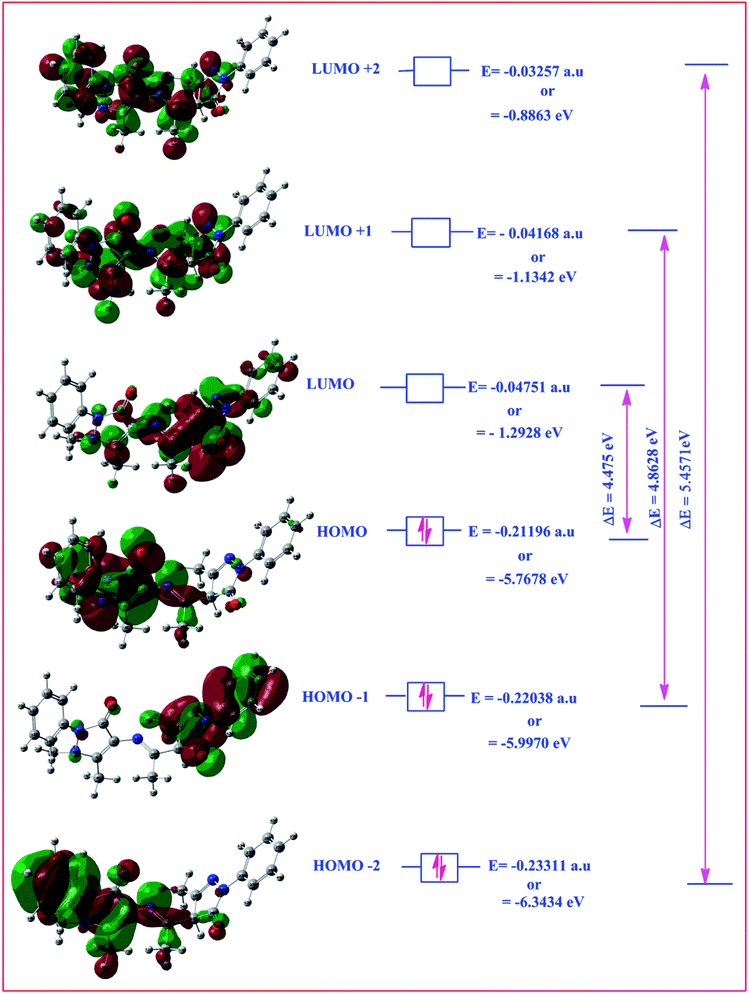 |
| | Fig. 13 HOMO–LOMO structure with energy level diagram of ligand II. | |
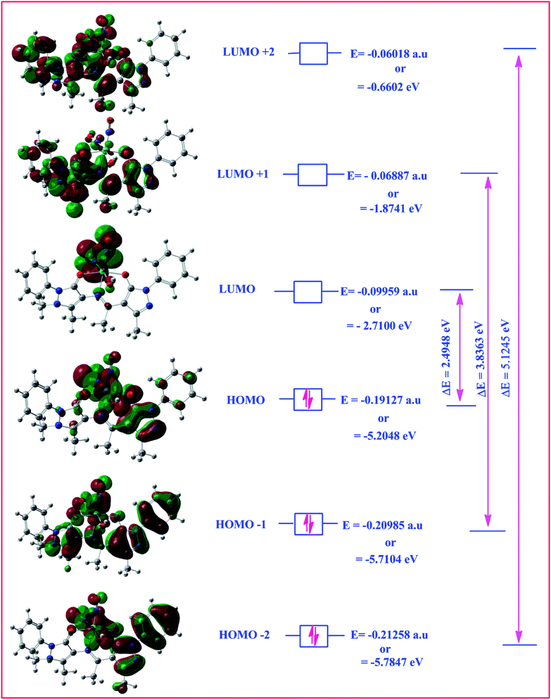 |
| | Fig. 14 HOMO–LOMO structure with energy level diagram of complex 2. | |
The energy of the frontier orbitals for molecules in term of ionization energy (IE) and electron affinity (IA) of the (amphp-aapH) and its complex are fetchable according to Koopmans's theorem.84 Similarly, the absolute electro negativity (χabs) and absolute hardness (η) are related to IA and EA.85 Hard molecules characterize a large HOMO–LUMO gap, and soft molecules show narrow gap.85 The absolute electro negativity (χabs), absolute hardness (η), electrophilicity index (ω) and global softness (S) of the two selected model compounds calculated so far are represented in Table 9.
Table 9 Absolute electronegativity (χabs), absolute hardness (η), electrophilicity index (ω), global softness (S) of (amphp-aapH) (II) and complex [Mo(NO)2(amphp-aap)(OH)] (2)
| Compounds |
χabs (eV) |
η (eV) |
ω (debye per eV) |
S (eV) |
μ (debye) |
| (amphp-aapH) |
3.5303 |
2.2375 |
14.0057 |
0.4469 |
7.9168 |
| [Mo(NO)2(amphp-aap)(OH)] |
3.9574 |
1.2474 |
72.9611 |
0.8017 |
13.4916 |
Antimicrobial study
The antimicrobial activity of the representative complex 1 was tested against some Gram negative, Gram positive and fungal strains of microbes including Pseudomonas, E. coli, Streptococcus and Aspergillus, by agar well diffusion method. The inhibition zones in millimeters of shown by the model complex are given in Table 10. IC50 values of the complex indicate that it has good degree of antimicrobial properties. IC50 values of 128 against Streptococcus, 134 against Pseudomonas, 288 against E. Coli and 219 against Aspergillus have been found. The Petriplates displaying the inhibition zones have been shown in Fig. 15. The increase in the biological activity of the metal complexes can be explained on the basis of chelation theory and overtones concept.86–88 According to chelation theory, the delocalization of π electrons over the whole chelate ring enhances the lipophilicity and the polarity of the metal atom is reduced due to the overlap of the ligand orbital and partial share of positive charge of metal atom with ligands.89–91 So, increase in lipophilic character results in an increase in permeability through the lipid layers of cell membrane and the metal binding sites on enzymes of microorganism are blocked. Overtone's concept is based on cell permeability, wherein the lipid membrane that surrounds the cell favours the passage of only the lipophilic materials due to which lipo-solubility is an important factor, which controls the antimicrobial action.92 It is observed that different compounds show antimicrobial activity of low variation range against bacterial and fungal species. This difference depends either on the impermeability of the cells of the microorganism which, in case of Gram positive is single layered and in the case of Gram negative is multilayered structure or differences in ribosomes of microbial cells. It can possibly be concluded that the chelation increased the activity of these complexes. The present results show that dinitrosyl molybdenum Schiff base complexes possess better cytotoxicity than the corresponding Schiff base ligand against the same microbes. Although the complexes are active, they did not reach the effectiveness of the conventional bactericide ofloxacin and fungicide fluconazole. However, it may be mentioned that the activity index (A.I.) given against each concentration, Fig. 16, showing excellent biological effects in case of the complex:
Table 10 Antimicrobial screening of [Mo(NO)2(dha-aap)(H2O)]
| Strain |
ZIa and AIa at 100 μg mL−1 con. |
ZI and AI at 75 μg mL−1 con. |
ZI and AI at 50 μg mL−1 con. |
1 μg mL−1 (std.) |
| ZI |
AI |
ZI |
AI |
ZI |
AI |
| Z. I. is the zone of inhibition and A. I. is the activity index at the particular concentration of the sample. |
| Streptococcus |
42.75 |
0.91 |
39.0 |
0.83 |
31.25 |
0.67 |
46.75(Ofloxacin) |
| Pseudomonas |
41.50 |
0.92 |
37.0 |
0.82 |
29.75 |
0.66 |
45.25(Ofloxacin) |
| E. coli |
24.50 |
0.74 |
21.50 |
0.65 |
17.75 |
0.53 |
33.25(Ofloxacin) |
| Aspergillus |
26.50 |
0.85 |
22.50 |
0.72 |
16.75 |
0.54 |
31.0(Fluconazole) |
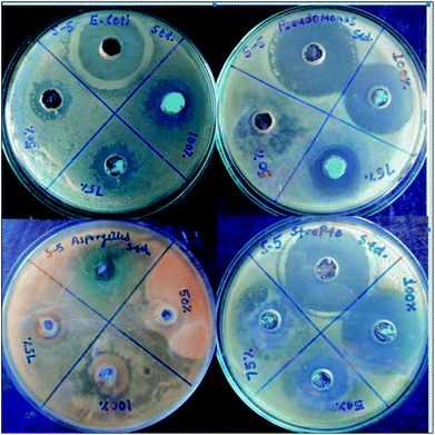 |
| | Fig. 15 Petri-plates showing zones of antimicrobial actions at different concentrations by the complex 1. | |
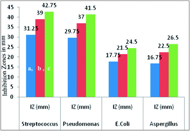 |
| | Fig. 16 Graphical presentation of inhibition zones against the particular strains at different concentrations (a = 50 μg mL−1, b = 75 μg mL−1 and c =100 μg mL−1) shown by complex 1. | |
It is noteworthy to state here that the inhibition zones were shown to have remarkably increased on increasing the concentration of the compounds under investigation.
Antiproliferative effects on colo-205 human cancer cells
Expression of nitric oxide in cancerous cells triggered the possible applications of nitrosyl complexes in treating cancer. In the present investigation the selected cancer cell line is related with the dreadful colon cancer which is the second most common cause of cancer-related death after lung cancer. Literature survey shows that risk parameters confined to nutrition and genes result in additive effects of the tumor. On other hand the co-relation of NO (nitric oxide) with apoptosis induction upon COLO 205 represents important asset of the targeted theme. Antiproliferative tests were carried out separately for ligand I and its respective complex using MTT assay.93 Doxorubicin with 2% dimethylsulfoxide (DMSO) was used as standard control. Fig. 17 shows the exhibited dose-dependent antiproliferative activity against colo-205 human cancer cells of the target compounds and significantly reduced the growth rate of colo-205 cancer cells. It has been shown that the dinitrosyl complex of molybdenum bears better cytotoxic activity as compared to the corresponding Schiff base. The related data of cell inhibition and cell survival have been given in Table 11. From IC50 values 53.13 in the Schiff base and 10.51 in its complex, it is established that latter bears more anticancer potentiality. Both the biological assays are found supportive in the assumption that the complexes bears better biological relevance as compared to the free ligands. The reasons lying behind this factual observation can be explained on the basis of theoretical results also. Electron density plots and charge populations analysis are the tools which help to build up insights regards the potential characteristics of a molecule.94,95
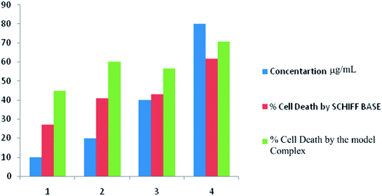 |
| | Fig. 17 Dose dependant anti-proliferative data of the model compounds I and 1. | |
Table 11 Antiproliferative data of (dha-aapH) ligand and its dinitrosyl complex
| |
Control absorbance |
Concentration μg mL−1 |
Absorbance |
% cell survival |
% cell death |
| (dha-aapH) |
1.21 |
10 |
0.118 |
90.24 |
27.11 |
| 20 |
0.284 |
76.53 |
40.83 |
| 40 |
0.311 |
74.30 |
43.06 |
| 80 |
0.536 |
55.70 |
61.65 |
| [Mo(NO)2(dha-aap)(OH)] (I) |
1.47 |
10 |
0.188 |
87.21 |
44.76 |
| 20 |
0.243 |
83.47 |
60.27 |
| 40 |
0.360 |
75.51 |
56.46 |
| 80 |
0.421 |
71.36 |
60.61 |
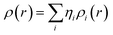
Molecular charge analysis and electron density plots as biological speculative tools
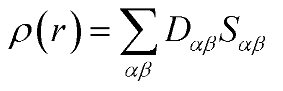
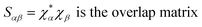
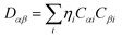
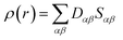
Drug/medicinal properties depicted by compounds are mainly focused with regard to lipophilicity, size and charge analysis. Depending on the electronic charge on the chelating atoms one may depict the bonding capability of a molecule. In order to quantify and compare specific interactions pertaining to the pictorial presentation of orbitals, numerical values serve as the keys to intensify their value. In case of donation versus back donation in transition metals and σ/π bonding it may prove helpful by assigning charges to the constituent atoms of a molecule. Pictorial presentation of orbitals are instant informative, however for the purpose to quantify and compare specific interactions numerical values are the keys to intensify the informative representation.96–99 For instance, donation versus back donation in transition metal complexes, single, double and triple bonding in organic compounds. Assigning charges to atoms is very useful idea for performing a rough idea of charge distribution in a molecule. The total electron density is expanded in terms of molecular orbitals and then each orbital can be extrapolated in terms of a set of atomic orbitals (the basis set).| |
 | (xxi) |
 and ηi accounts for the orbital occupation
| |
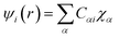 | (xxii) |
So,| |
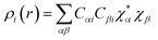 | (xxiii) |
So,| |
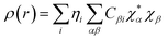 | (xxiv) |
If we interchange the summation indices, which basically means we change the order in which we sum up all the individual terms:
| |
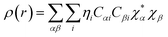 | (xxv) |
| |
 | (xxvi) |
is the density matrix and we write
ρ(
r) in a simplified form,
| |
 | (xxvii) |
Population analysis methods divide up DαβSαβ to obtain numbers that tell us where the electron density in a system resides. A few of more common wave function population analyses methods include Mulliken, Lowdin, Roby, Mayer, Cioslowski, Charge decomposition analysis (CDA) and Natural Bond Order (NBO).100–105
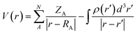
Population methods also assign each atom a partial charge. Each atom centre is positively charged core (charge ZA) surrounded by shielding electron, once we know how much electron density each atom has we can determine the atomic partial charge
| | |
qA = ZA − ∫ρA(r)dr
| (xxviii) |
However, there is a problem; the charge can be distributed in different ways by different methods qualitatively. As there is no observable property associated with the “partial charge” and also there isn't any reference value to which computed values can be compared. Thus there is also no way to evaluate the accuracy. It is very important not to over interpret data provided by population methods as partial charges are artificial, they do not present an observable property of atoms or molecules.
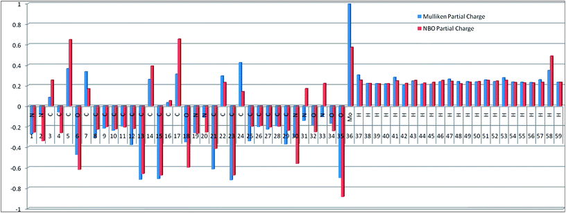
One localization ad population analysis method that very popular is the natural bond order analysis. In this method natural atomic orbitals that are effective orbitals of an atom in the particular molecular environment (rather than isolated or in gas phases) are determined. There are also the maximum occupancy orbitals. NBOs are localized at few centre MOs that reflect Lewis like bonding structure. The natural atomic charges of a representative complex, [Mo(NO)2(amphp-aap)(OH)] obtained by NBO and Mulliken population analysis with B3LYP/LANL2DZ basis set are compared in Fig. 18. The comparison between Mulliken's net charges and the atomic natural ones is not an easy task since the theoretical background of the two methods was very different. Looking at the results there are surprising differences between the Mulliken's and the NBO charges. The observation of the data of the complex 2 shows that the atoms namely C3, C5, C7, C14, C16, C17,C22, C24, Mo36 and all hydrogen bear positive charge both in NBO and Mulliken analyses. The remaining atoms possess negatively charges over them in both the analysis. It is noticeable that N33 atom of one of the two NO ligands, is negatively charged in Mulliken scale but has positive partial charge in NBO analysis. This demonstrates the redistribution of charges when compared with the NPA analysis of representative Schiff base.
| |
 | (xxix) |
 |
| | Fig. 18 Graphical presentation of Mulliken and NBO population analysis of complex 2. | |
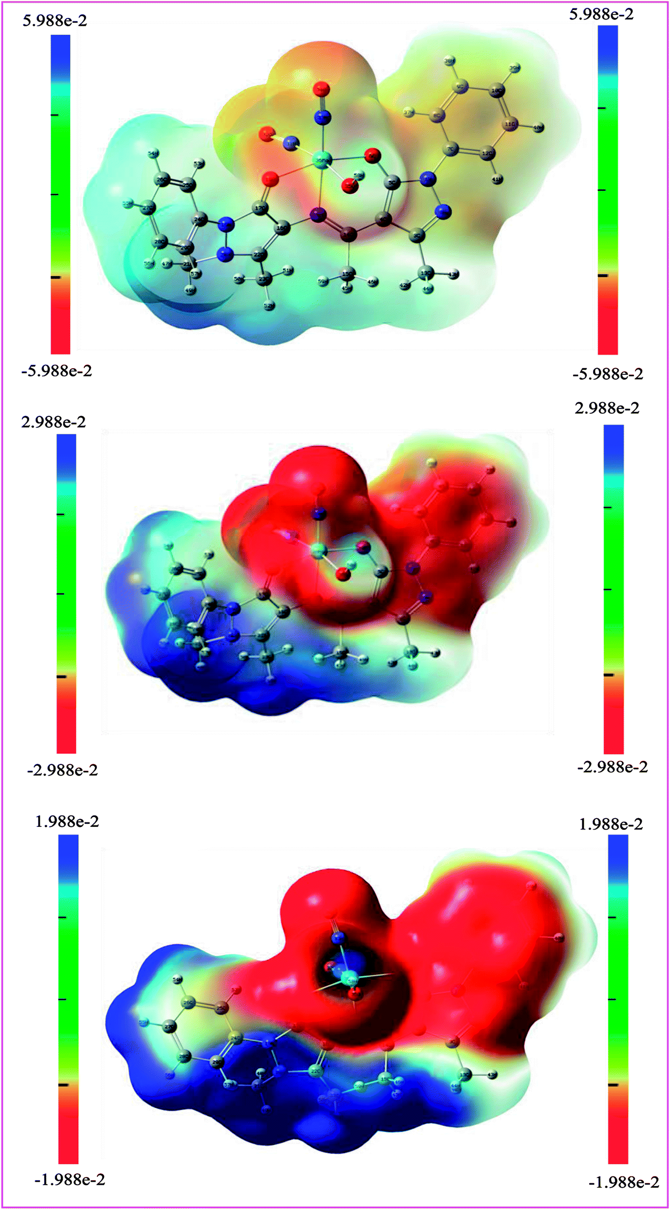
The MESP diagram is used to understand the interactive behavior of a molecule, in that negative regions can be regarded as nucleophilic centers, whereas the positive regions are potential electrophilic sites. The molecular electrostatic potentials of the model complex is given in Fig. 19, displaying molecular shape, size and electrostatic potential values. The MESP map of the complex indicates the coordination sphere is the region of most negative potential. The hydrogen and nitrogen atoms in a ligand bear the region of maximum positive charge. It is noteworthy here that the two hydrogens attached to the electronegative oxygen of the coordinated water molecule are most electropositive. The predominance of green region in the MESP surfaces corresponds to a potential halfway between the two extremes red and dark blue color.106 A scheme has been developed by changing numerical assignment decreased by one unit, a stage reached when the two most electropositive and the most electronegative region become quite distinctive as shown in Fig. 19.
 |
| | Fig. 19 Electron density plot and incremental distinction of highly electropositive and highly electronegative regions of complex 2. | |
Conclusions
The comparative experimental and theoretical study of pyrazolone Schiff base dinitrosylmolybdenum(0) complexes revealed that the complexes bear a cis-octahedral geometry. The experimental and theoretical data were found in excellent agreement with one another. The evaluation of thermal chemistry using different methods indicate the Freeman Carrol method exhibits quite different readings as compared with other three methods regarding the TG-based kinetic and thermodynamic studies. In vitro anticancer and antimicrobial actions also exhibited high potent anticancer and antimicrobial activity of the compounds. Overall, the investigation suggests that the compounds reported so far are good future tools to be biologically tested against more virulent diseases.
Conflicts of interest
No conflict(s) of interest is declared by the authors.
Acknowledgements
The authors thankfully acknowledge Vice Chancellor, R. D. University Jabalpur, India, for his support in developing the lab infrastructure. SAIF, IIT Mumbai, UGC networking Centre Hyderabad Central University, PBRI, Bhopal, Food Science Department Kashmir University and IIT, Chennai are also gratefully acknowledged for rendering necessary lab facilities.
References
- A. Fejzic and S. Cavar, Bull. Chem. Technol. Bosnia Herzegovina, 2014, 42, 1–4 Search PubMed.
- J. Wang, R. P. Woldring, G. D. Roman-Melendez, A. M. McClain, B. R. Alzua and E. N. G. Marsh, ACS Chem. Biol., 2014, 9, 1929–1938 CrossRef CAS PubMed.
- P. Hanzelmann and H. Schindelin, Proc. Natl. Acad. Sci. U. S. A., 2004, 101, 12870–12875 CrossRef PubMed.
- P. Hanzelmann, G. Schwarz and R. R. Mendel, J. Biol. Chem., 2002, 277, 18303–18312 CrossRef CAS PubMed.
- R. C. Maurya and J. M. Mir, Int. J. Appl. Sci. Eng. Res., 2014, 5, 282–321 Search PubMed.
- J. M. Mir, S. Roy, P. K. Vishwakarma and R. C. Maurya, J. Chin. Adv. Mater. Soc., 2018, 6, 282–300 Search PubMed.
- S. M. O. Quintal, H. I. S. Nogueira, H. M. Carapuca, V. Felix and M. G. B. Drew, J. Chem. Soc., Dalton Trans., 2001, 0, 3196–3201 RSC.
- L. Lisnard, P. Mialane, A. Dolbecq, J. Marrot and F. Secheresse, Inorg. Chem. Commun., 2003, 6, 503–505 CrossRef CAS.
- B. Modec, J. V. Brencic, E. M. Burkholder and J. Zubieta, Dalton Trans., 2003, 0, 4618–4625 RSC.
- R. Villanneau, R. Delmont, A. Proust and P. Gouzerh, Chem.–Eur. J., 2000, 6, 1184–1192 CrossRef CAS.
- L. J. Csanyi, J. Mol. Catal. A: Chem., 2010, 322, 1–6 CrossRef CAS.
- R. Hille, Chem. Rev., 1996, 96, 2757–2816 CrossRef CAS PubMed.
- M. Nair, L. H. Nair and D. Thankamani, J. Serb. Chem. Soc., 2011, 76, 221–233 CrossRef CAS.
- T. Yonemura, J. Nakata, M. Kadoda, M. Hasegawa, K. Okamoto, T. Ama, H. Kawaguchi and T. Yasui, Inorg. Chem. Commun., 2001, 4, 661–663 CrossRef CAS.
- T. Yonemura, T. Hashimoto, M. Hasegawa, T. Ikenoue, T. Ama and H. Kawaguchi, Inorg. Chem. Commun., 2006, 9, 183–186 CrossRef CAS.
- T. Yonemura, Acta Crystallogr., 2009, 65, 1463–1464 Search PubMed.
- A. Sen and R. R. Thomas, Organometallics, 1982, 1, 1251–1254 CrossRef CAS.
- A. Keller and R. Matusiak, J. Mol. Catal., 1999, 142, 317–324 CrossRef CAS.
- A. Keller, J. Mol. Catal., 1993, 78, 15–18 CrossRef.
- A. Keller and R. Matusiak, J. Mol. Catal., 1996, 104, 213–219 CrossRef CAS.
- D. D. Thomas, C. Corey, J. Hickok, Y. Wang and S. Shiva, Redox Biol., 2018, 15, 277–283 CrossRef CAS PubMed.
- L. T. Elrod and E. Kim, Inorg. Chem., 2018, 57, 2594–2602 CrossRef CAS PubMed.
- F. Caron, M. Rivallan, S. Humbert, A. Daudin, S. Bordiga and P. Raybaud, J. Catal., 2018, 361, 62–72 CrossRef CAS.
- L. L. Thomson, F. G. Lawton, R. G. Knowles, J. E. Basley, V. Riversomoreno and S. Moncada, Cancer Res., 1994, 54, 1352–1354 Search PubMed.
- S. Taysi, C. Uslu, F. Akcay and M. Y. Sutbeyaz, Surg. Today, 2003, 33, 651–654 CrossRef CAS PubMed.
- C. S. Cabs, J. E. Brenman, K. D. Aldape, D. S. Bredt and M. A. Isrnael, Cancer Res., 1995, 55, 727–730 Search PubMed.
- S. Reveneau, L. Arnould, G. Jolimoy, S. Hilpert, P. Lejeune, V. Saint-Giorgio, C. Belichard and J. F. Jeannin, Lab. Invest., 1999, 79, 1215–1225 CAS.
- J. Prazma, P. Pertrusz, W. Mims, S. S. Ball and M. C. Weissler, Otolaryngol.--Head Neck Surg., 1995, 113, 541–549 Search PubMed.
- D. X. West, S. B. Padhye and P. B. Sonawane, Struct. Bonding (Berlin), 1991, 76, 1–50 CrossRef CAS.
- A. Mortensen and J. Lykkesfeldt, Nitric Oxide, 2014, 36, 51–57 CrossRef CAS PubMed.
- S. Majumder, S. Sinha, J. H. Siamwala, A. Muley, H. R. Seerapu, G. K. Kolluru, V. Veeriah, S. Nagarajan, S. R. C. Sridhara, M. K. Priya, M. Kuppusamy, S. Srinivasan, S. Konikkat, G. Soundararajan, S. Venkataraman, U. Saran and S. Chatterjee, Nitric Oxide, 2014, 36, 76–86 CrossRef CAS PubMed.
- A. C. B. A. Wanschel, V. M. Caceres, A. I. S. Moretti, A. B. Cardoso, H. F. de Carvalho, H. P. de Souza, F. R. M. Laurindo, R. C. Spadari and M. H. Krieger, Nitric Oxide, 2014, 36, 58–66 CrossRef CAS PubMed.
- M. Bahra, V. Kapil, V. Pearl, S. Ghosh and A. Ahluwalia, Nitric Oxide, 2012, 26, 197–202 CrossRef CAS PubMed.
- C. H. Hu and D. R. Chong, Chem. Phys. Lett., 1996, 262, 733–736 CrossRef CAS.
- L. C. J. Thomas, W. C. Bauschlicher Jr and B. M. Hall, J. Phys. Chem. A, 1997, 101, 8530–8539 CrossRef.
- M. Zhou and L. Andrews, J. Phys. Chem. A, 2000, 104, 3915–3925 CrossRef CAS.
- D. Bykov, M. Plog and F. Neese, J. Biol. Inorg Chem., 2014, 19, 97–112 CrossRef CAS PubMed.
- A. S. Azizyan, T. S. Kurtikyan, G. G. Martirosyan and P. C. Ford, Inorg. Chem., 2013, 52, 5201–5205 CrossRef CAS PubMed.
- G. F. Caramori, A. G. Kunitz, D. F. Coimbra, L. C. Garcia and D. E. P. Fonseca, J. Braz. Chem. Soc., 2013, 24, 1487–1496 CAS.
- P. F. Wu, S. C. Liu, Y. J. Shieh, T. S. Kuo, G. H. Lee, Y. Wang and Y. C. Tsai, Chem. Commun., 2013, 49, 4391 RSC.
- F. Neese, J. Biol. Inorg. Chem., 2006, 11, 702–711 CrossRef CAS PubMed.
- J. P. Perdew, Phys. Rev. B, 1986, 33, 8822–8824 CrossRef.
- A. D. Becke, J. Chem. Phys., 1986, 8, 4524–4529 CrossRef.
- W. A. Zoubi, S. G. Mohamed, A. A. S. Al-Hamdani, A. P. Mahendradhany and Y. G. Ko, RSC Adv., 2018, 8, 23294–23318 RSC.
- W. A. Zoubi, F. Kandil and M. K. Chebani, Arabian J. Chem., 2016, 9, 626–632 CrossRef.
- W. A. Zoubi, F. Kandil and M. K. Chebani, Spectrochim. Acta, Part A, 2011, 79, 1909–1914 CrossRef CAS PubMed.
- M. Shaharyar, A. A. Siddiqui, M. A. Ali, D. Sriram and P. Yogeeswari, Bioorg. Med. Chem. Lett., 2006, 16, 3947–3949 CrossRef CAS PubMed.
- J. F. Li, B. Guan, D. X. Li and C. Dong, Spectrochim. Acta, Part A, 2007, 68, 404–408 CrossRef CAS PubMed.
- G. Bai, J. Li, D. Li, C. Dong, X. Han and P. Lin, Dyes Pigm., 2007, 75, 93–98 CrossRef CAS.
- Z. Lu, Q. Jiang, W. Zhu, M. Xie, Y. Hou, X. Chen and Z. Wang, Aust. J. Chem., 2005, 27, 2267–2274 Search PubMed.
- N. A. Evans, D. E. Rivett and J. F. K. Wilshire, Aust. J. Chem., 2005, 27, 2267–2274 CrossRef.
- B. S. Jensen, Acta Chem. Scand., 199, 13, 1668–1670 CrossRef.
- R. C. Maurya, A. Pandey, J. Chaurasia and H. Martin, J. Mol. Struct., 2006, 798, 89–101 CrossRef CAS.
- W. B. Taylor, Biometrics, 1957, 13, 1–12 CrossRef.
- T. Mosmann, J. Immunol. Res., 1983, 65, 55–63 CAS.
- L. R. Holloway, A. J. Clough, J. Y. Li, E. L. Tao, F. Tao and L. Li, Polyhedron, 2014, 70, 29–38 CrossRef CAS PubMed; M. J. Frisch, G. W. Trucks, H. B. Schlegel, G. E. Scuseria, M. A. Robb, J. R. Cheeseman, G. Scalmani, V. Barone, B. Mennucci, G. A. Petersson, H. Nakatsuji, M. Caricato, X. Li, H. P. Hratchian, A. F. Izmaylov, J. Bloino, G. Zheng, J. L. Sonnenberg, M. Hada, M. Ehara, K. Toyota, R. Fukuda, J. Hasegawa, M. Ishida, T. Nakajima, Y. Honda, O. Kitao, H. Nakai, T. Vreven, J. A. Montgomery, Jr, J. E. Peralta, F. Ogliaro, M. Bearpark, J. J. Heyd, E. Brothers, K. N. Kudin, V. N. Staroverov, T. Keith, R. Kobayashi, J. Normand, K. Raghavachari, A. Rendell, J. C. Burant, S. S. Iyengar, J. Tomasi, M. Cossi, N. Rega, J. M. Millam, M. Klene, J. E. Knox, J. B. Cross, V. Bakken, C. Adamo, J. Jaramillo, R. Gomperts, R. E. Stratmann, O. Yazyev, A. J. Austin, R. Cammi, C. Pomelli, J. W. Ochterski, R. L. Martin, K. Morokuma, V. G. Zakrzewski, G. A. Voth, P. Salvador, J. J. Dannenberg, S. Dapprich, A. D. Daniels, O. Farkas, J. B. Foresman, J. V. Ortiz, J. Cioslowski and D. J. Fox, Gaussian 09, Revision C.01, Gaussian, Inc., Wallingford CT, 2010 Search PubMed.
- GaussView 9.0, Gaussian Inc., Garnegie Office Park, Pittsburgh. PA, USA Search PubMed.
- S. Bayari, S. Saglan and H. F Ustundag, J. Mol. Struct.: THEOCHEM, 2005, 726, 225–232 CrossRef CAS.
- J. Jayabharathi, V. Thanikachalam and M. V. Perumal, Spectrochim. Acta, Part A, 2012, 95, 614–621 CrossRef CAS PubMed.
- R. C. Maurya, D. D. Mishra, S. Mukherjee and P. K. Trivedi, Transition Met. Chem., 1991, 16, 524–527 CrossRef CAS.
- R. C. Maurya, D. D. Mishra, N. S. Rao and N. N. Rao, Synth. React. Inorg. Met.-Org. Chem., 1994, 24, 1013–1025 CrossRef CAS.
- R. C. Maurya, D. D. Mishra, N. S. Rao and N. N. Rao, Bull. Chem. Soc. Jpn., 1995, 68, 1589–1592 CrossRef.
- R. C. Maurya and V. Pillai, Indian J. Chem., 1999, 38A, 736–739 CAS.
- R. C. Maurya, J. Dubey and B. Shukla, Synth. React. Inorg. Met.-Org. Chem., 1998, 28, 1159–1171 CrossRef CAS.
- S. Sarkar, R. C. Maurya and S. C. Chaurasia, Transition Met. Chem., 1976, 1, 49 CrossRef CAS.
- D. Gwost and K. G. Caulton, Inorg. Chem., 1974, 13, 414–417 CrossRef CAS.
- M. P. Perpinan, L. Ballester, A. Santos and A. Monge, Polyhedron, 1987, 6, 1523–1532 CrossRef CAS.
- W. J. Geary, Coord. Chem. Rev., 1971, 7, 81–122 CrossRef CAS.
- J. H. Enemark and R. D. Feltham, in Topics in Inorganic and Organometallic Stereochemistry, ed. G. Geoffroy, Wiley, New York, 1981, vol. 12, pp. 152–215 Search PubMed.
- M. E. Brown, Introduction to Thermal Analysis: Techniques and Applications, Springer Science, 2001, DOI:10.1007/0-306-48404-8.
- H. B. Singh, S. Maheshwari and H. Tomer, Thermochim. Acta, 1983, 64, 47–53 CrossRef CAS.
- K. K. Srivastavaa, S. Srivastavab and Md. T. Alam, Int. J. Pharma Bio Sci., 2013, 2, 26–37 Search PubMed.
- P. P. Kalbende, M. V. Tarase and A. B. Zade, J. Chem., 2012, 2013 DOI:10.1155/2013/846327.
- E. S. Freeman and B. Carroll, J. Phys. Chem., 1958, 62, 394–397 CrossRef CAS.
- H. H. Horowitz and G. Metzger, Anal. Chem., 1963, 35, 1464–1468 CrossRef CAS.
- A. W. Coats and I. P. Redfern, Nature, 1964, 20, 68–69 CrossRef.
- A. Broido, J. Polym. Sci., Part A-2, 1969, 7, 1761–1773 CrossRef CAS.
- A. A. Frost and R. G. Pearson, Kinetics and Mechanism, J. Chem. Educ., 1961, 38, P535 Search PubMed.
- P. B. Maravalli and T. R. Goudar, Thermochim. Acta, 1999, 325, 95–105 CrossRef.
- K. K. M. Yusuf and R. Sreekala, Thermochim. Acta, 1990, 159, 357–368 CrossRef.
- D. B. Brown, E. G. Walton and J. A. Dits, J. Chem. Soc., Dalton Trans., 1980, 845–850 RSC.
- D. Shoba, S. Periandy, M. Karabacak and S. Ramalingam, Spectrochim. Acta, Part A, 2012, 83, 540–552 CrossRef PubMed.
- K. Fukui, Science, 1982, 218, 747–754 CrossRef CAS PubMed.
- C. J. Brabec, N. S. Sariciftci and J. C. Hummelen, Adv. Funct. Mater., 2001, 11, 15–26 CrossRef CAS.
- E. E. Ebenso, T. Arslan, F. Kandemirli, I. Love, M. Saracoglu and S. A. Umoren, Int. J. Quantum Chem., 2010, 110, 2614–2636 CrossRef CAS.
- A. H. Kianfar, L. Keramat, M. Dostani, M. Shamsipur, M. Roushani and F. Nikpour, Spectrochim. Acta, Part A, 2010, 77, 424–429 CrossRef PubMed.
- A. A. Nejo, G. A. Kolawole and A. O. Nejo, J. Coord. Chem., 2010, 63, 4398–4410 CrossRef CAS.
- N. Raman, S. Sobha and A. Thamaraichelvan, Spectrochim. Acta, Part A, 2011, 78, 888–898 CrossRef CAS PubMed.
- T. Rosu, E. Pahontu, C. Maxim, R. Georgescu, N. Stanica and A. Gulea, Polyhedron, 2011, 30, 154–162 CrossRef CAS.
- N. Raman, A. Kulandaisamy, C. Thangaraja and K. Jeyasubramanian, Transition Met. Chem., 2003, 28, 29–36 CrossRef CAS.
- R. Karvembu, C. Jayabalakrishnan, N. Dharmaraj, S. V. Renukadevi and K. Natarajan, Transition Met. Chem., 2002, 27, 631–638 CrossRef CAS.
- Y. Anjaneyulu and R. P. Rao, Synth. React. Inorg. Met.-Org. Chem., 1986, 16, 257–272 CrossRef CAS.
- J. M. Mir, N. Jain, P. S. Jaget and R. C. Maurya, Photodiagn. Photodyn. Ther., 2017, 19, 363–374 CrossRef CAS PubMed.
- J. M. Mir and R. C. Maurya, J. Chin. Adv. Mater. Soc., 2018, 6, 156–168 CrossRef CAS.
- J. M. Mir and F. A. Itoo, J. Mol. Liq., 2017, 247, 1–5 CrossRef CAS.
- R. S. Mulliken, J. Chem. Phys., 1955, 23, 1833–1840 CrossRef CAS.
- J. M. Mir, P. K. Vishwakarma and R. C. Maurya, J. Chin. Adv. Mater. Soc., 2018, 6, 55–80 CrossRef CAS.
- R. C. Maurya, B. A. Malik, J. M. Mir, P. K. Vishwakarma, D. K. Rajak and N. Jain, J. Coord. Chem., 2015, 68, 2902–2922 CrossRef CAS.
- J. M. Mir, N. Jain, P. S. Jaget, W. Khan, P. K. Vishwakarma, D. K. Rajak, B. A. Malik and R. C. Maurya, J. King Saud Univ., Sci., 2017 DOI:10.1016/j.jksus.2017.06.006 , in press.
- J. M. Mir, N. Jain, B. A. Malik, R. Chourasia, P. K. Vishwakarma, D. K. Rajak and R. C. Maurya, Inorg. Chim. Acta, 2017, 467, 80–92 CrossRef CAS.
- J. M. Mir, R. C. Maurya and P. K. Vishwakarma, Karbala Int. J. Mod. Sci., 2017, 3, 212–223 CrossRef.
- R. C. Maurya, B. A. Malik, J. M. Mir, P. K. Vishwakarma, D. K. Rajak and N. Jain, J. Mol. Struct., 2015, 1099, 266–285 CrossRef CAS.
- R. C. Maurya, B. A. Malik, J. M. Mir and P. K. Vishwakarma, J. Mol. Struct., 2015, 1083, 343–356 CrossRef CAS.
- P. K. Vishwakarma, J. M. Mir and R. C. Maurya, J. Chem. Sci., 2016, 128, 511–522 CrossRef CAS.
- J. M. Mir, R. C. Maurya, D. K. Rajak, B. A. Malik, P. S. Jaget and N. Jain, Karbala Int. J. Mod. Sci., 2017, 3, 153–164 CrossRef.
- R. C. Maurya, B. A. Malik, J. M. Mir and A. K. Sharma, J. Coord. Chem., 2014, 67, 3084–3106 CrossRef CAS.
Footnote |
| † Electronic supplementary information (ESI) available: Refer supplemental material for Tables S1–S13 and Fig. S1–S9. See DOI: 10.1039/c8ra05956j |
|
| This journal is © The Royal Society of Chemistry 2018 |
Click here to see how this site uses Cookies. View our privacy policy here. 
 Open Access Article
 This Open Access Article is licensed under a Creative Commons Attribution-Non Commercial 3.0 Unported Licence
 * and
Ram Charitra Maurya
* and
Ram Charitra Maurya
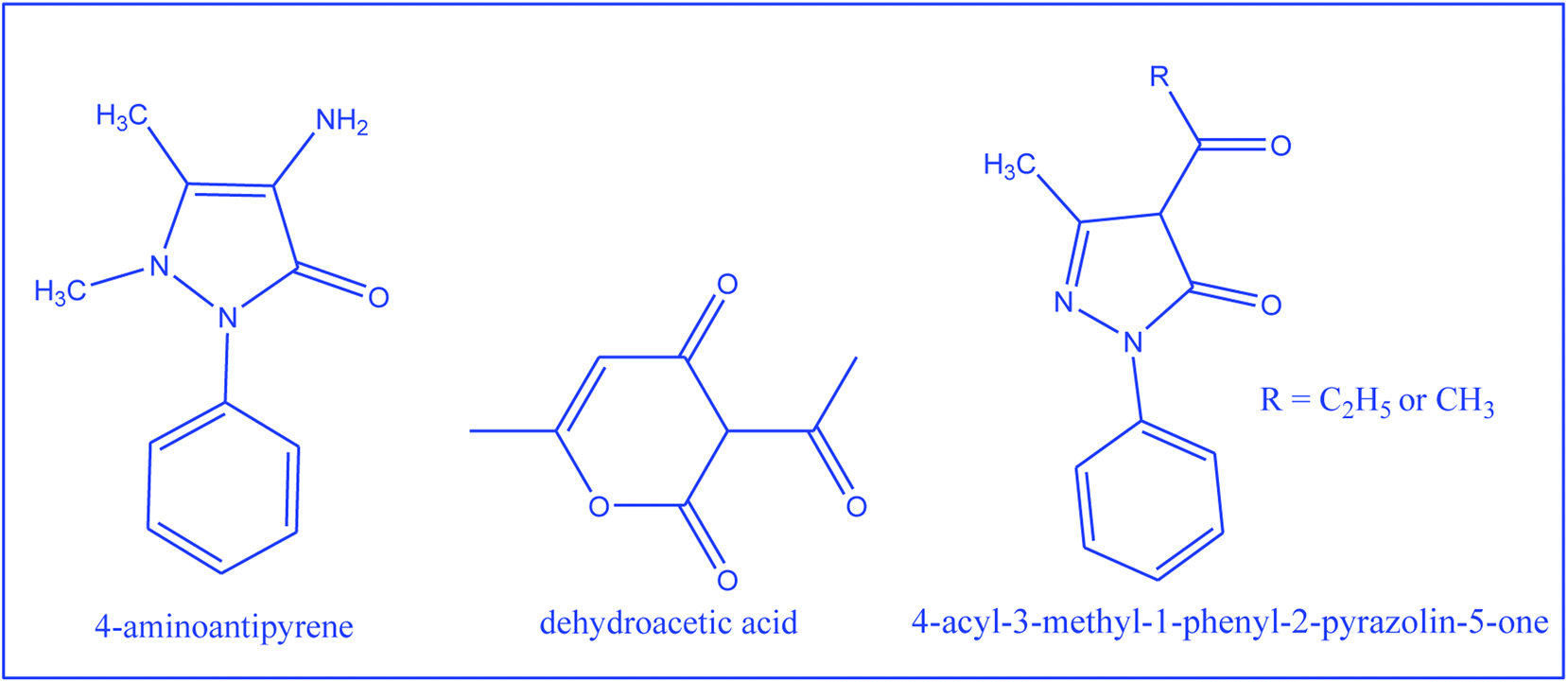
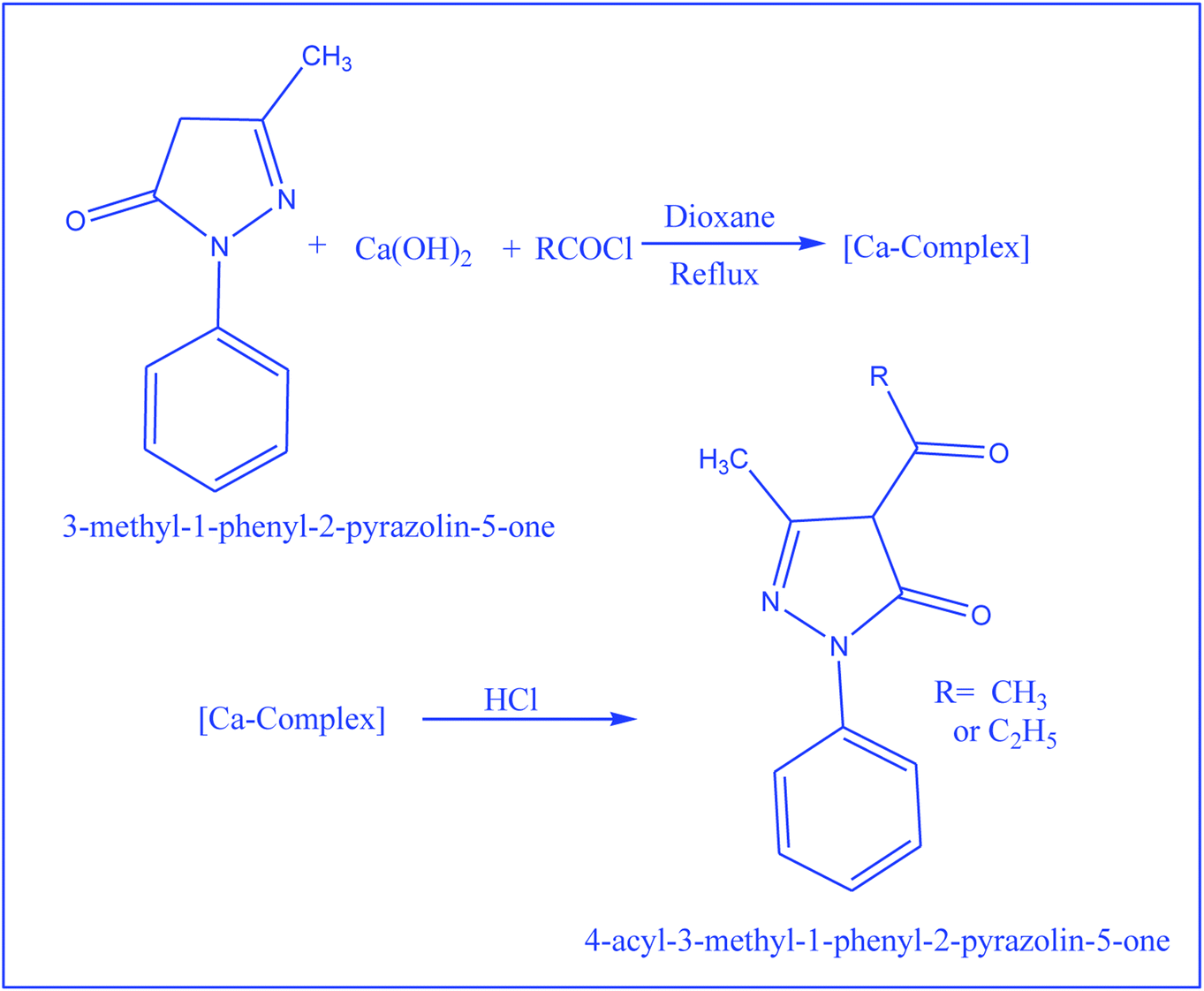

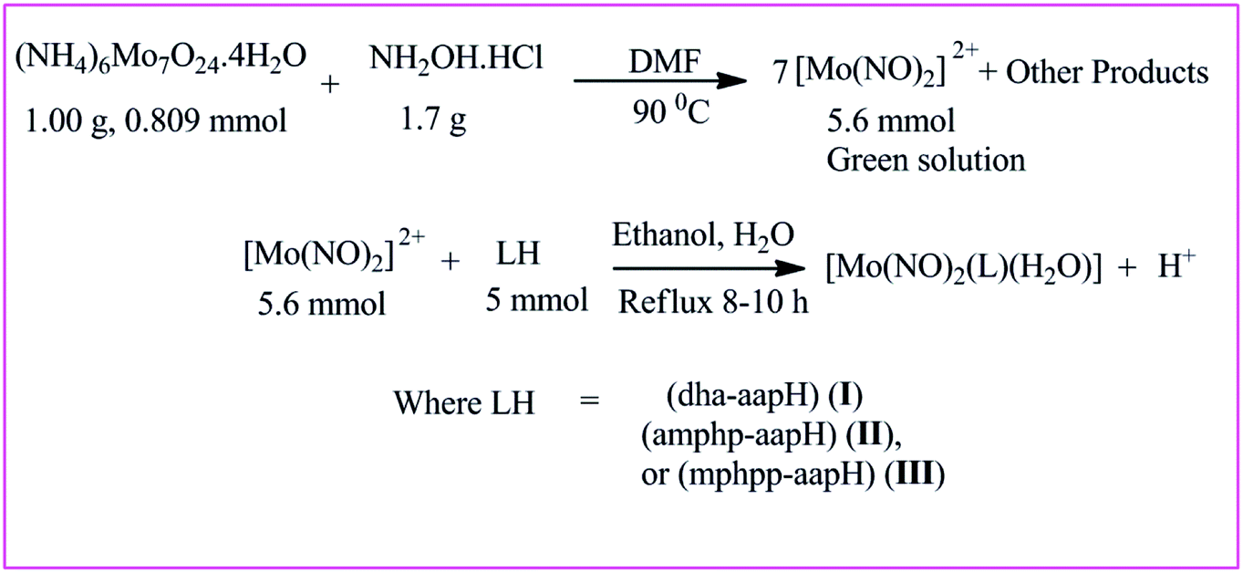
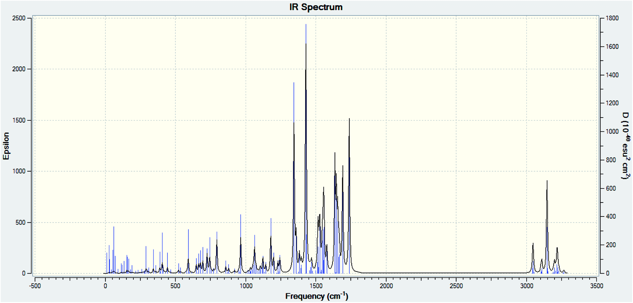
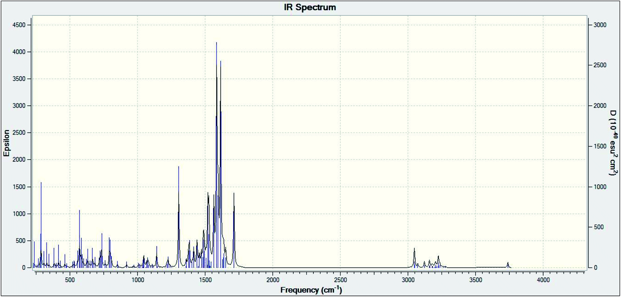
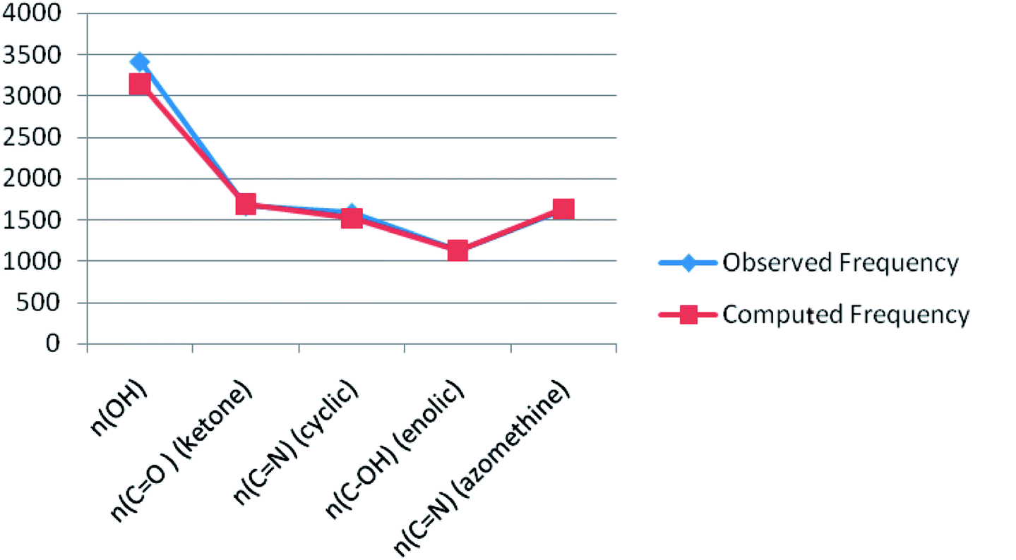
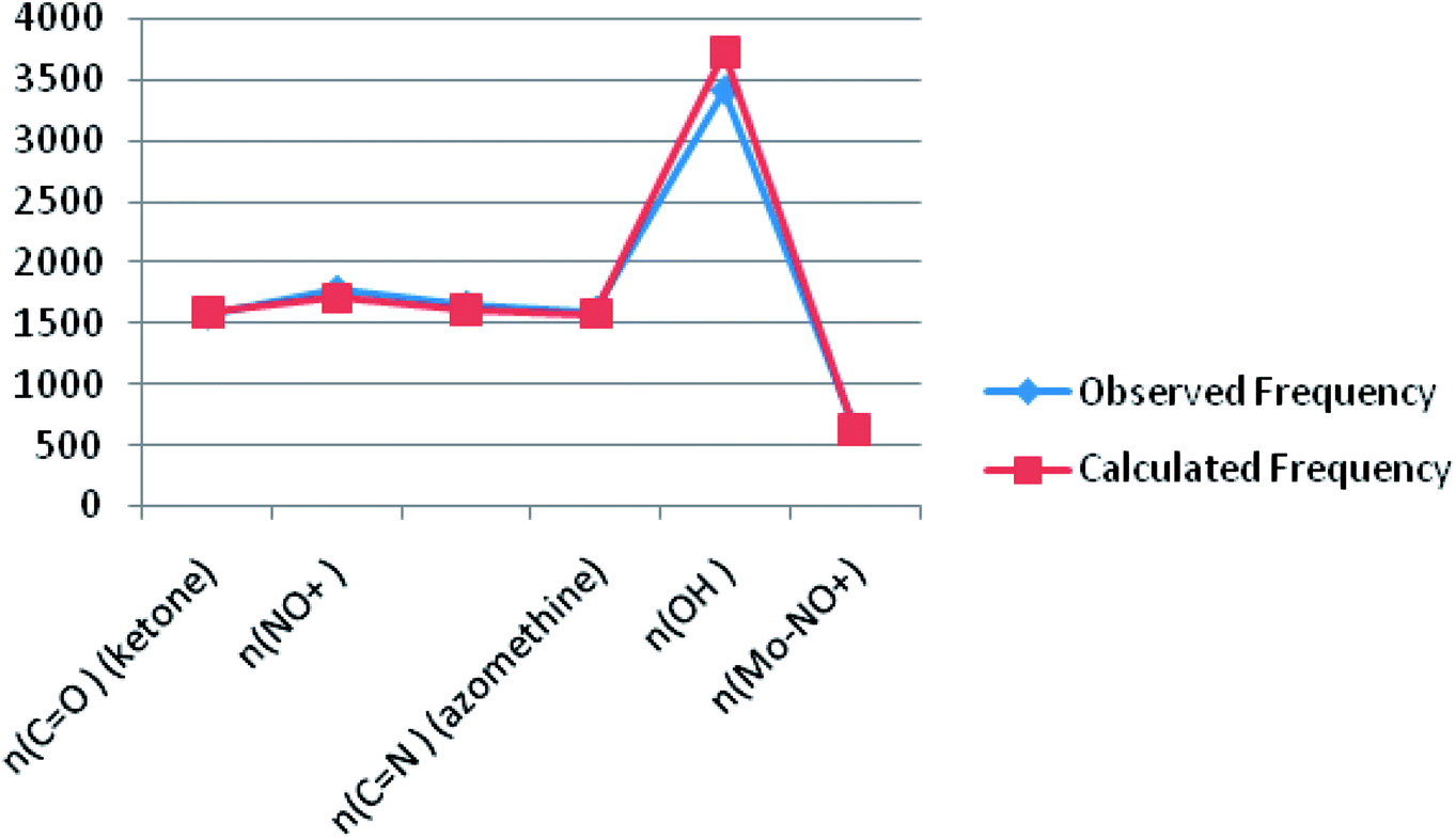
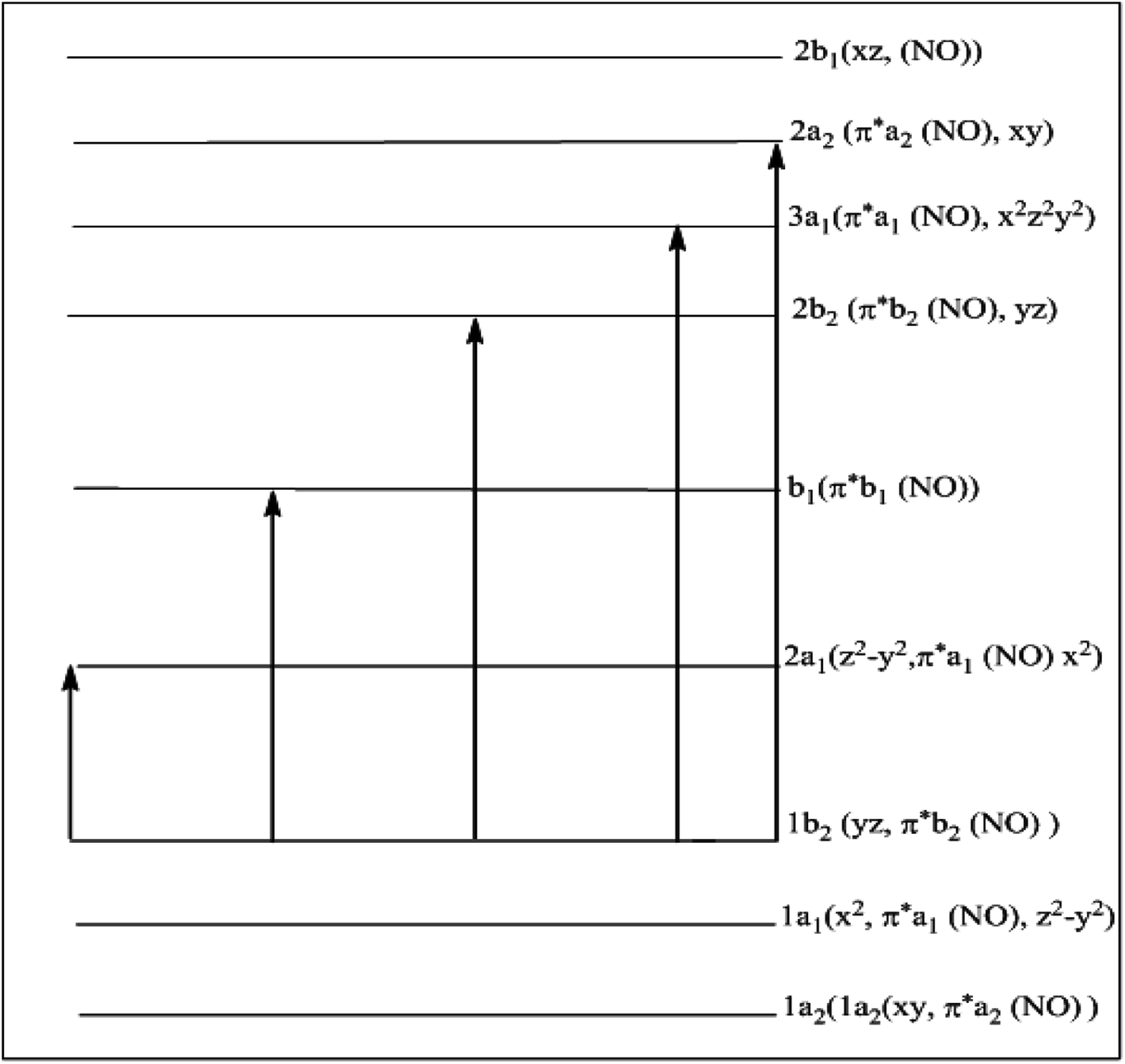


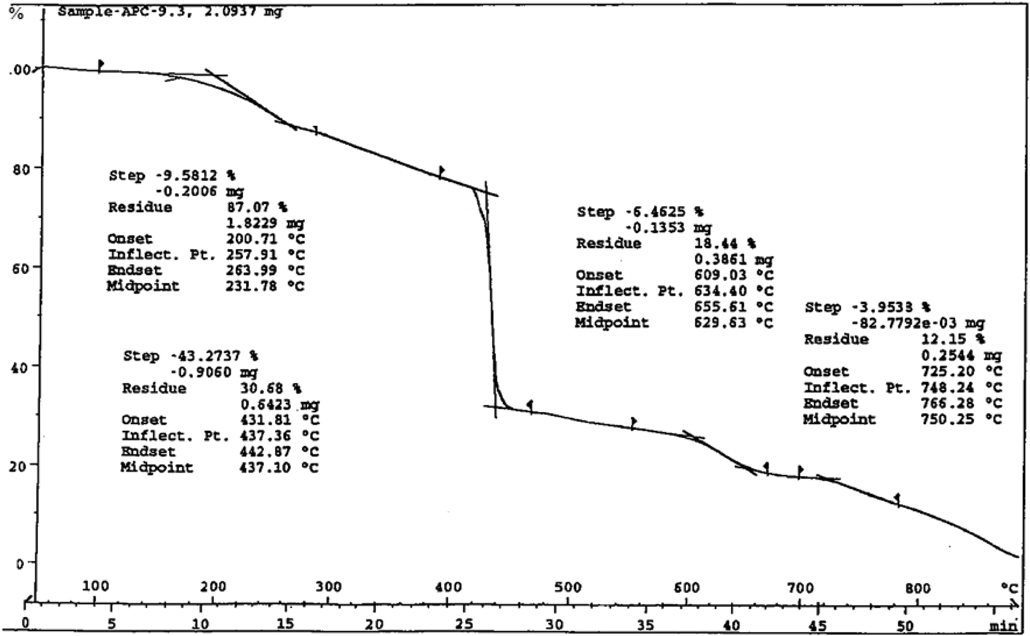
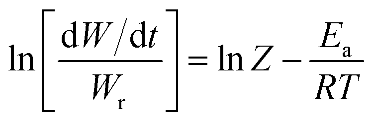
 against 1/T should be linear for decomposition following 1st order kinetics. The slope of plot gives the value of Ea, while the intercept is equal to ln
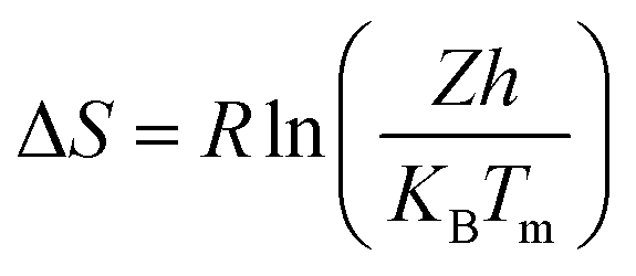
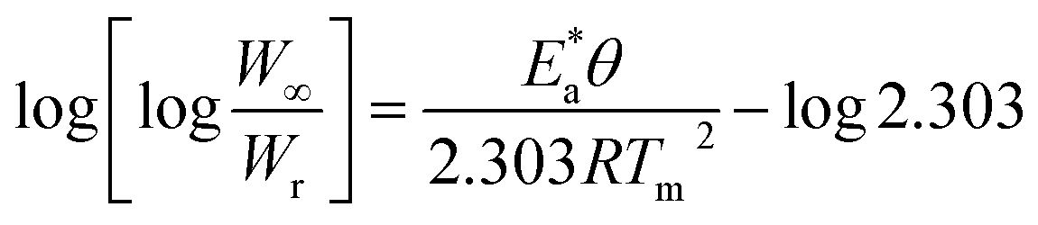
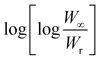 against θ should gives a straight line with slope
 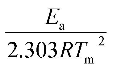 , from which from which Ea can be obtained. The frequency factor Z may be calculated using equation as
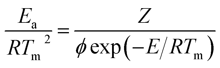
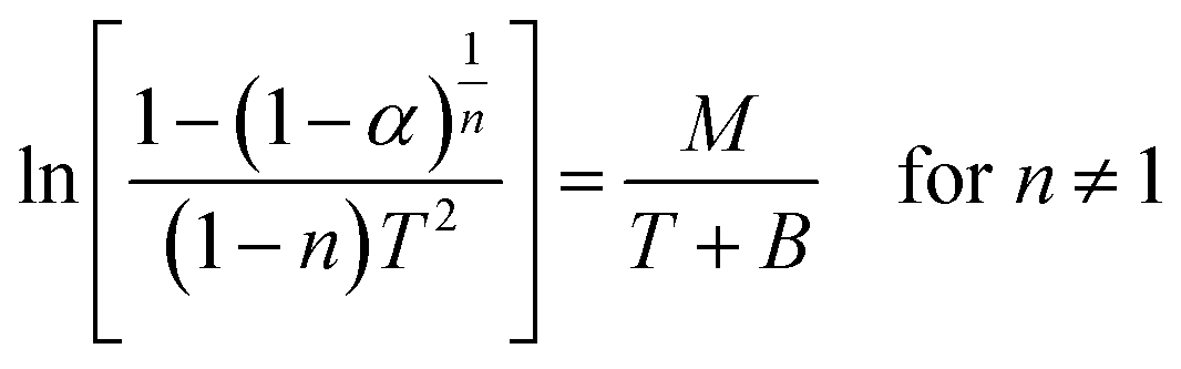
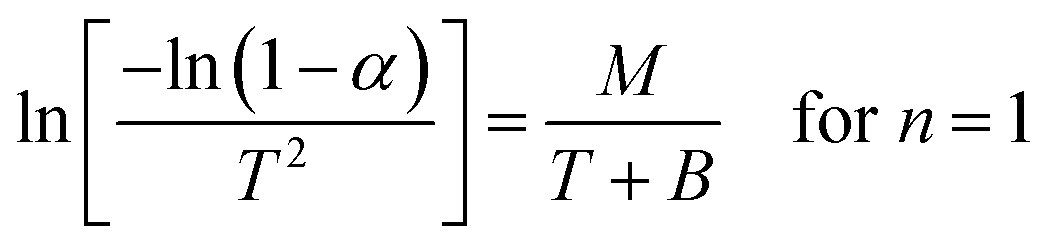
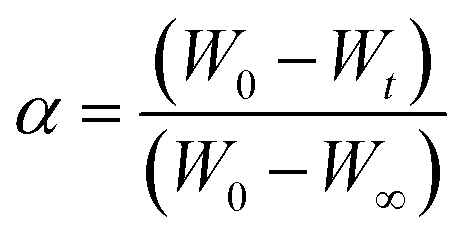
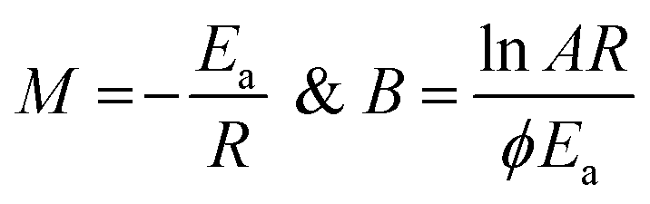
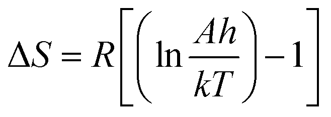
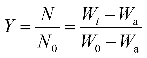
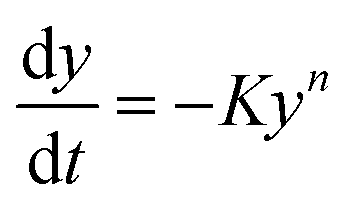
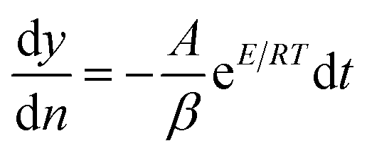

 vs. 1/T yields straight line, whose slope is directly related to Ea:
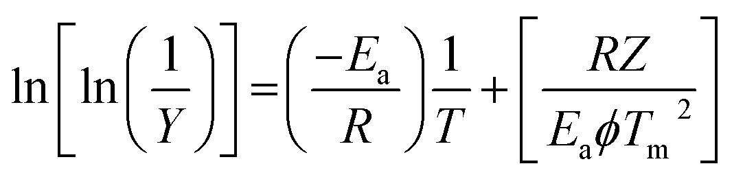
 and Z can be calculated from the relation
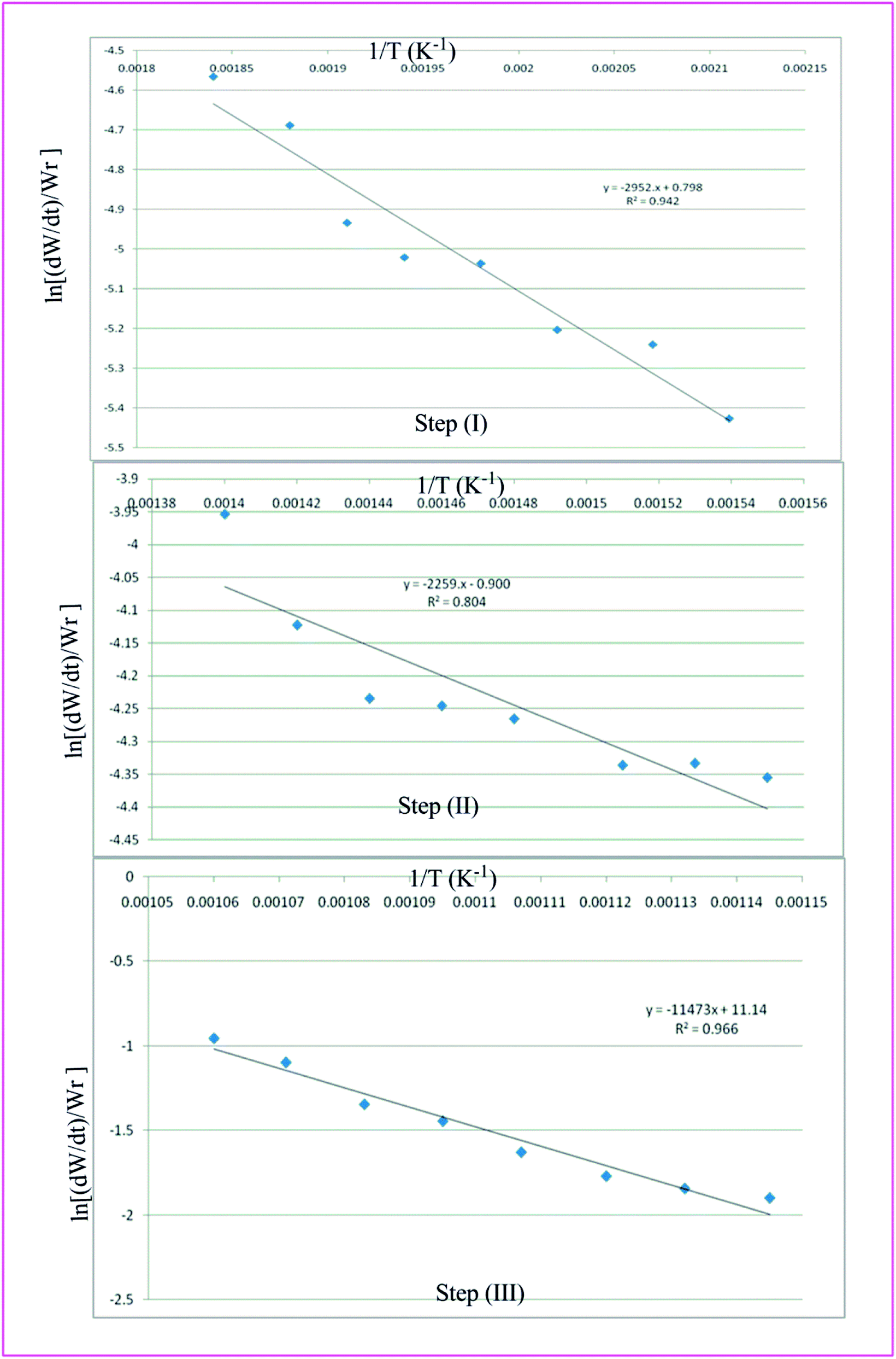

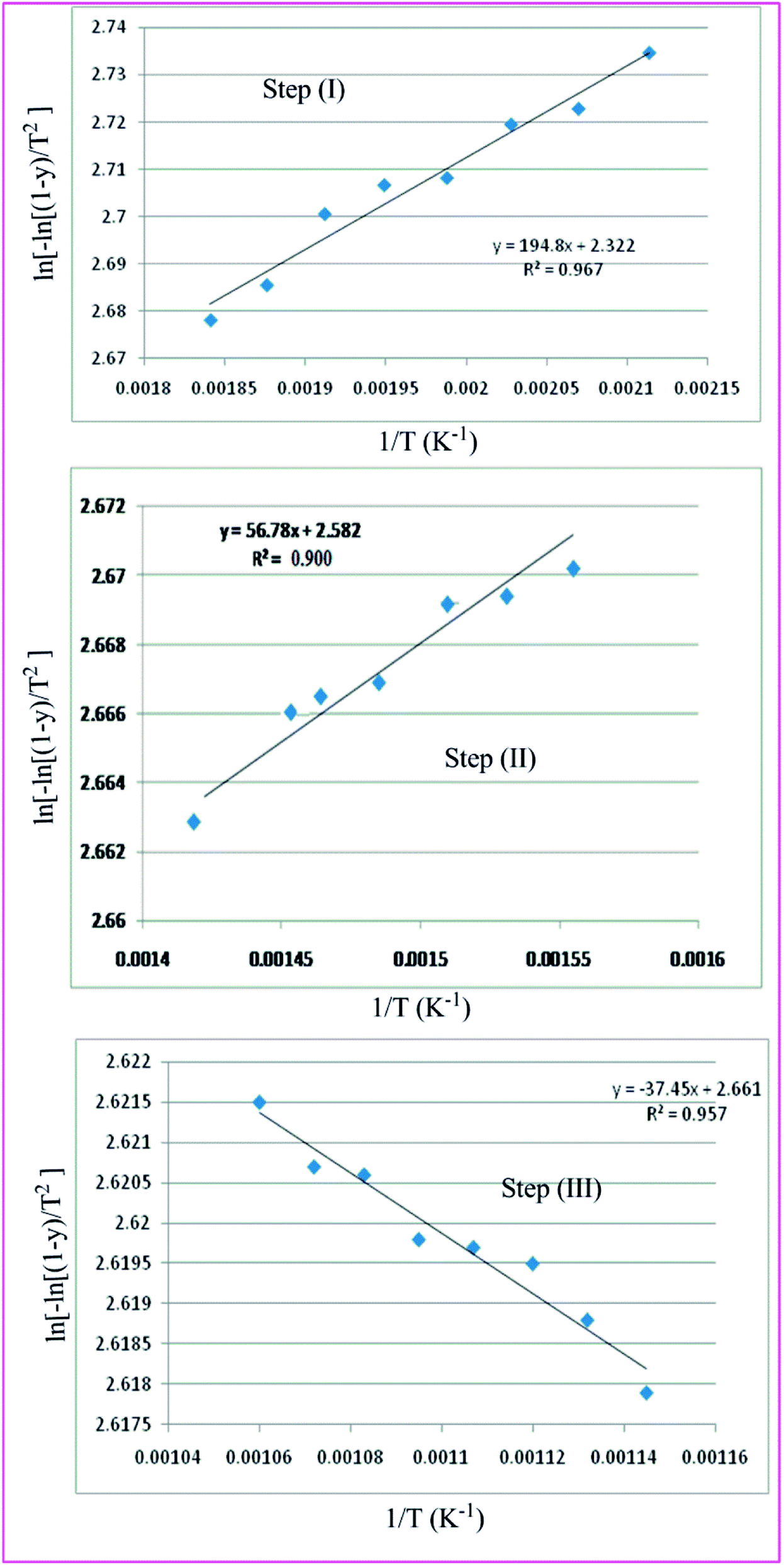
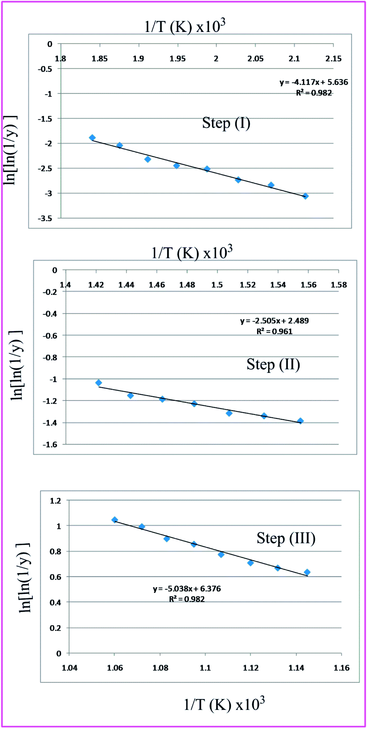

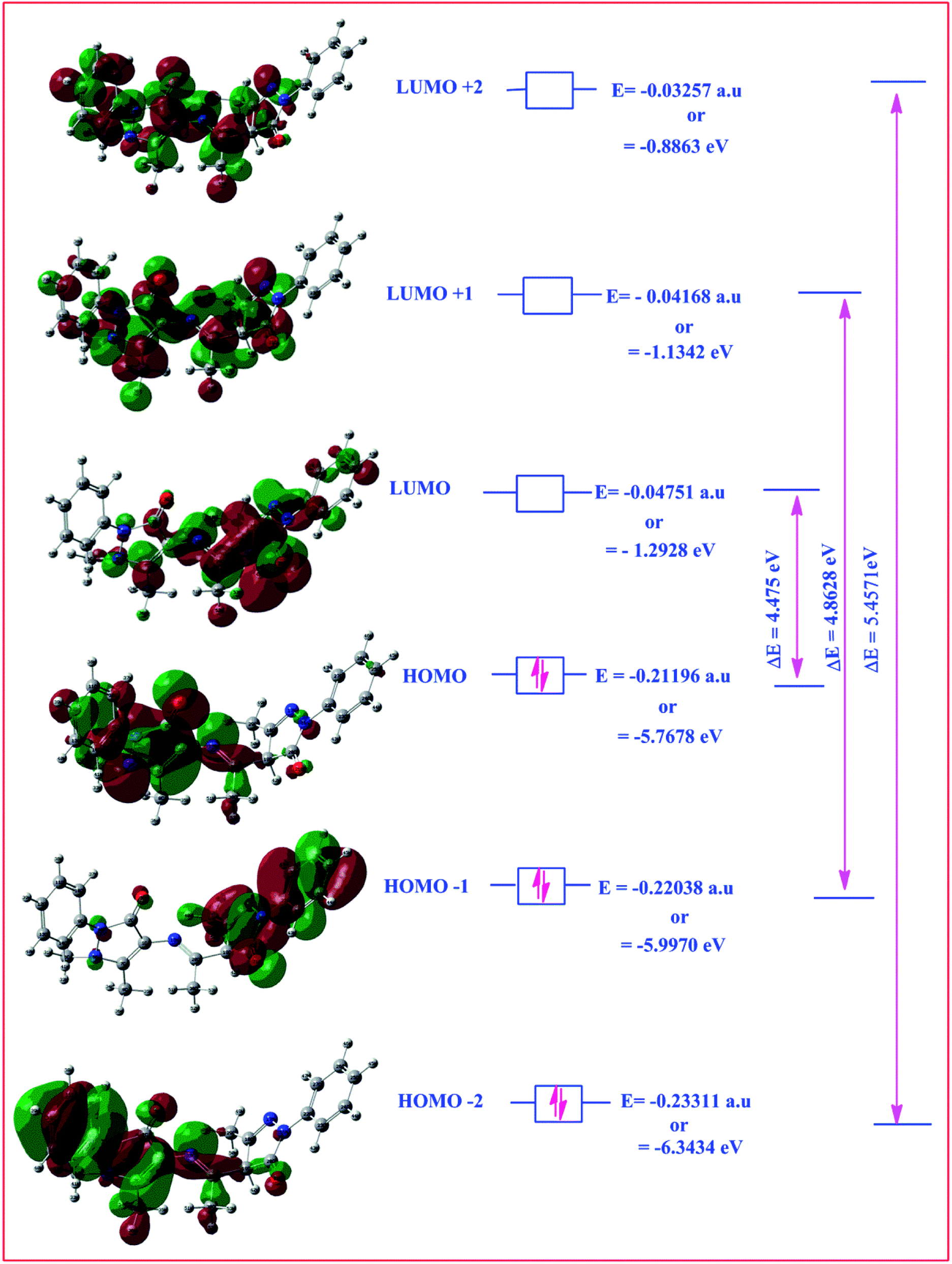
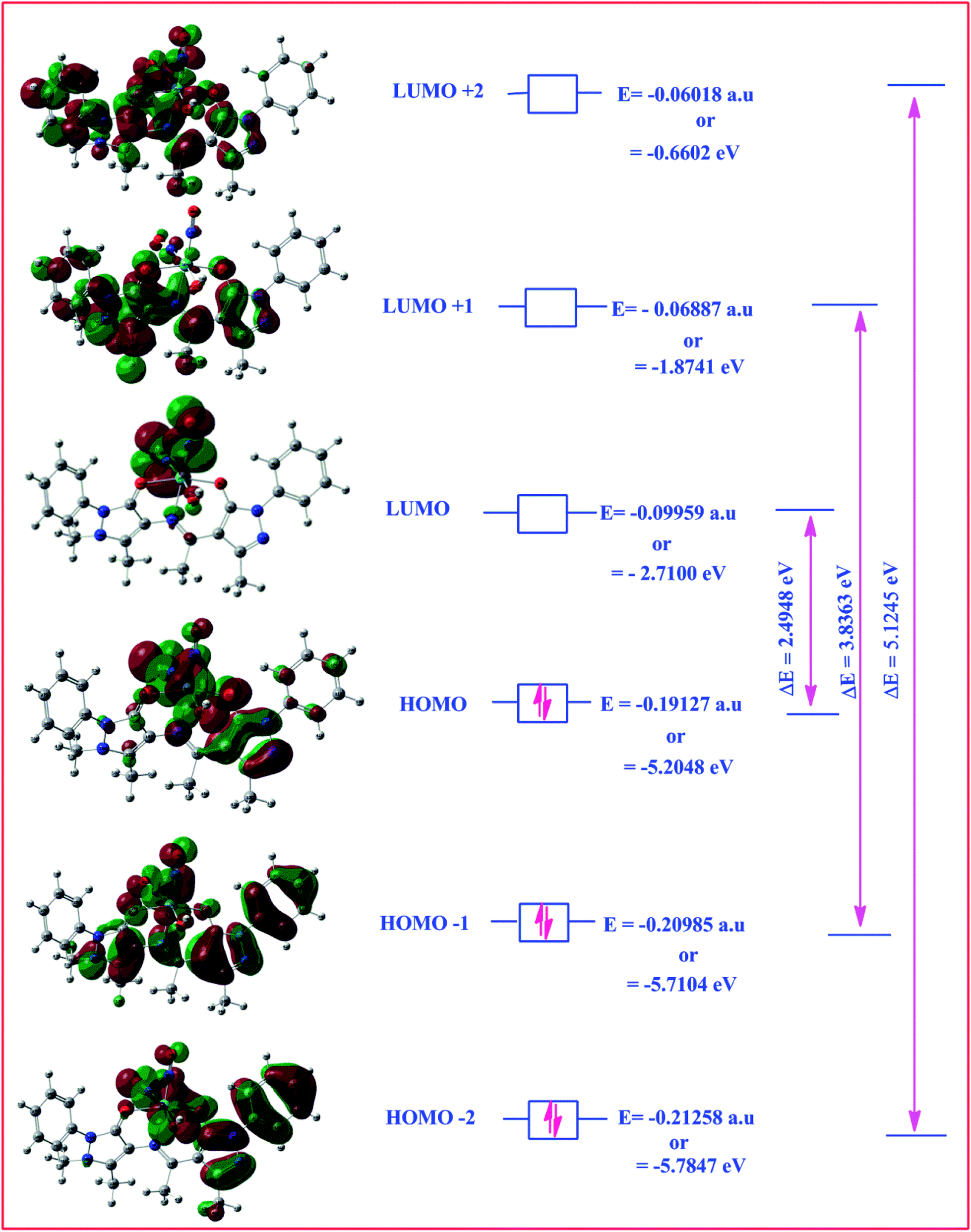
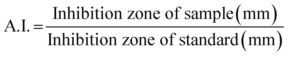

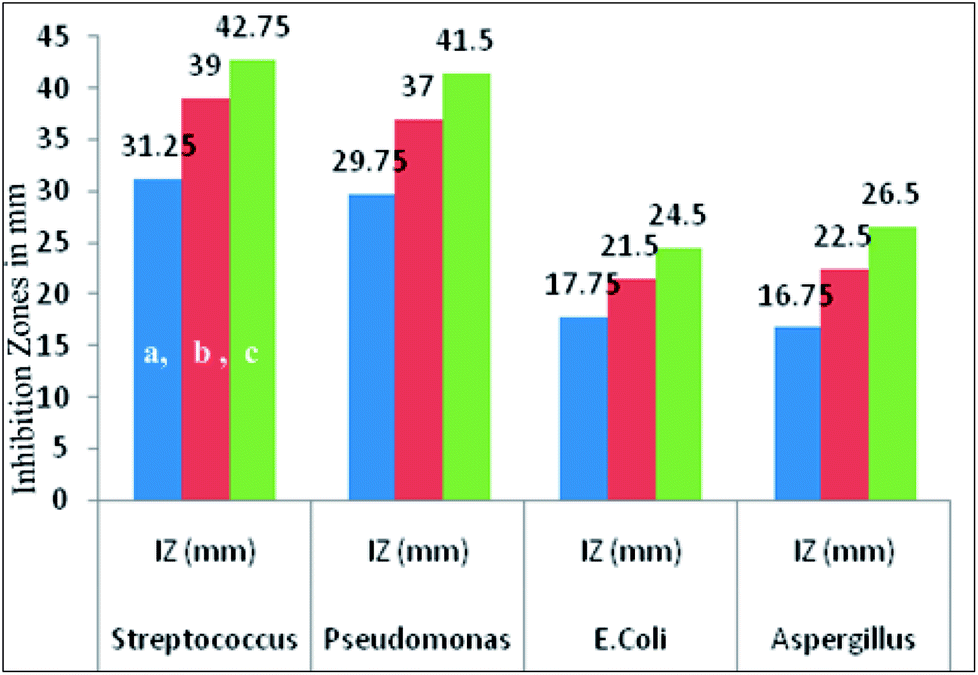

 and ηi accounts for the orbital occupation
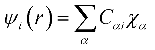
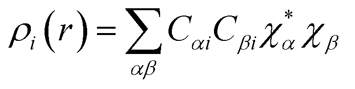
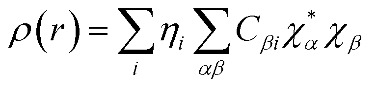
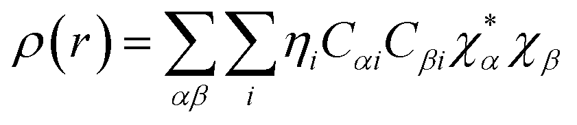
 is the density matrix and we write ρ(r) in a simplified form,