Heat transfer effect in scaling-up a fluidized bed reactor for propylene polymerization

Abstract

The effects of operating conditions and scaling-up on reactor temperature control and performance in propylene polymerization fluidized bed reactors were studied by phenomenological and CFD models. A phenomenological model with CFD hydrodynamics parameters predicts average information, while a CFD-based reactor model provides local information. Results suggest improved productivity and reactor temperature control by cautiously increasing catalyst feed rate, operating temperature, reactor size and superficial velocity, with consideration of hot spots and catalyst deactivation. High catalyst loading increases productivity but involves risk with regards to the control of oscillating temperature and hot spots. The model identifies an operating window to improve productivity and temperature control and to study operation details. Mixing effect is important to heat transfer but not to propylene conversion. Scaling-up cannot provide similarity of heat transfer. Keeping the same temperature when scaling up from 0.2 to 4 m in diameter requires heat transfer area multiplying factors of 2.43 to 5.26 or lowering the wall temperature by 7 to 18 K. Hot spots are detected with a temperature variation of 10 to 14 K. The results are useful for analyses of laboratory and industrial scale reactors and provide information on scale up.

---

1. Introduction

Polypropylene (PP) polymerization is usually operated in either three-phase slurry or gas fluidized reactors.¹ A slurry mode of operation provides good temperature control due to the liquid solvent being able to provide good heat transfer. However, by the nature of high viscosity of the slurry, the solid content has to be limited. Moreover, an additional evaporation unit is needed. In contrast, a gas-phase polypropylene polymerization fluidized bed is more attractive due to the fact that it can be operated with a high solid loading, requires neither drying nor separation of polymers from solvents and has relatively low environmental impact.^2,3 Nevertheless, heat transfer in a gas-phase fluidized bed is limited, especially in a high-solid-loading mode of operation, due to highly exothermic polymerization and poor heat transfer in the gas phase of the system. Thus, the bed temperature is difficult to control. The temperature of the polymer particles tends to rise, leading to particle overheating, sintering, catalyst deactivation, and loss of control over polymer product properties, including particle morphology. Polymer particles can melt and stick together to form bigger particles or fuse into a sheet or large chunk because the temperature in the reactor is greater than the melting point of the polymer. The fluidized bed operation can then approach a de-fluidized regime. A PP industrial fluidized bed reactor needs to shut down for clearing plastic chunks accumulated in the reactor over time. Thus temperature control is of primary concern to the overall reactor performance. The major challenges in this present work are to achieve faster reactions and higher production of PP with appropriate catalyst feed rate while retaining product quality and overcoming the heat transfer limitations. In addition, the problem of heat transfer limitation in reactor scaling up has to be focused on.

Models for fluidized bed reactors with reasonable simplifications are useful for this challenge. Two modeling approaches—phenomenological model and computational fluid dynamic based model—can be used for modeling the polymerization reactor. A phenomenological model is capable of predicting overall performance, i.e., monomer concentration, polymer production rate, bed temperature, molecular weight in a polymerization reactor as an averaged solution with reasonably computational time. However, the spatial variation of reactor performance cannot be obtained. Fortunately, the conversion of this reaction is in a low range, e.g., less than 10%.^3–5 This model, based on average bed phenomena, can thus sufficiently estimate the operating variables. However, the high degree of heat released from the exothermic polymerization reaction can cause a non-uniform temperature distribution, leading to hotspot generation. CFD-based reactor analysis is able to provide necessary information on the spatial distributions of phase movements and local temperature distribution.

Species balance of multiple components, heat transfer for both phases, and method of moments, can be used for predicting reactor performance by considering the hydrodynamic and transport parameters, which may be treated as constant values for simplicity. Several researchers^5–10 have applied a well-mixed model for polypropylene production. In the literature, the hydrodynamic parameters such as bed expansion and solid holdup were mainly obtained from the correlations based on Geldart A. Polymerization is usually carried out in a wide range of particle sizes, ranged from Geldart A to Geldart B. In addition, the reactor is operated at high temperature and pressure. The available correlations are usually based on cold models and in the regime of Geldart A. Thus the hydrodynamic parameters should be modified such that they better approximate real operating conditions. Hydrodynamics based on hot models obtained by CFD are required so as to obtain key parameters for accurate prediction of heat and mass transfer in a fluidized bed reactor.

Phenomenological models cannot provide local variation of temperature in the reactor, which is useful for monitoring hotspots and the possibility of polymer melting. CFD-based reactor analysis can capture local behavior of gas–solid in a fluidized bed reactor. The temperature distribution can be clearly explored by this model. An Eulerian–Eulerian approach to CFD has been successful to describe the hydrodynamics of gas–solid systems.^11–13 Xu et al. (2012)¹⁴ and Yao et al. (2014)¹⁵ applied CFD to polypropylene in a fluidized bed reactor. Li et al. (2016)¹⁶ used a computational fluid dynamics-discrete element model for studying temperature variation in fluidized beds. In their work, a constant heat source was added into the energy balance equation for the solid phase so as to mimic the propylene polymerization reaction heat. Temperature distribution and hotspots occurrence were found. The extension of Li et al.'s work considered here includes species balance for polymerization for non-uniformity of heat effect.

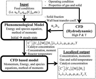
Combining the momentum, energy and species balances in the CFD models with the complex kinetic polymerization model as well as the method of moments can provide the distributions of solid holdup, temperature, polymerization conversion and polymer molecular weight. Although a CFD approach is useful to improve our understanding of this polymerization, it has a limitation in term of simulation time. Therefore, in this work, the limitation will be avoided by seperating the simulation into two levels of study. At the first level, a phenomenological model will be used to predict the overall performance in terms of monomer concentration, polymer production rate, bed temperature, and molecular weight in the polymerization reactor as an averaged solution. Subsequently, the solution obtained from the phenomenological model is used to provide the starting conditions for a CFD model. So as to get more detailed understanding, CFD will be used to provide additional information on local distributions of studied variables as well as hotspots in the fluidized bed reactor.

A heat transfer limitation problem can occur during reactor scaling up from a laboratory scale to industrial scale. To keep hydrodynamic similarity, Glicksman^17,18 proposed a set of non-dimensional parameters by non-dimensionalizing the governing equations of motion for the fluids and the solids in a fluidized bed. In addition, similarity in weight space time should be a criterion in order to have reactor performance similarity. These two criteria of similarities were used in the scaling-up work.

The aim of this work is to develop models at two levels and point out the utility of such an approach for carrying out simulations of a fluidized bed reactor for propylene polymerization. To improve productivity and change product properties, the operating variables studied are catalyst feed rate, operating temperature, hydrogen feed, reactor size and superficial velocity, and the sensitivity to operation window will be examined. In addition, local distributions of phase movements and local temperature distribution will be also studied in order to avoid polymer overheating, hot spots and possibility of polymer melting. The combination model presented in this work is unique and will be useful for improving the understanding of propylene polymerization in fluidized bed reactors and analysis both of a laboratory reactor and industrial reactor.

2. Mathematical model

Two models—a phenomenological model and a CFD-based model—are developed in this work. The phenomenological model is capable of predicting average monomer concentration, polymer production rate, bed temperature, and molecular weight in a polymerization reactor as an averaged solution. Meanwhile the CFD-based model is able to provide the local distributions of phase movements and the local temperature distribution. CFD simulation has a limitation in term of simulation time. Therefore, in this work, the phenomenological model is used to provide starting conditions for the CFD based model, as shown in Fig. 1. The phenomenological model is based on a well-mixed model which consists of energy balance, species balance for gas and solid phases and moment equations. The solid holdup and heat transfer parameters in this model were obtained from CFD hydrodynamic simulation based on high temperature and pressure conditions (see Fig. 1). The solutions for concentration of each species, concentration of catalyst, moments, and reactor temperature obtained from the phenomenological model were used to initialize the CFD-based model for local parameters studies.

Fig. 1 The schematic of coupling CFD and phenomenological model.

2.1 Phenomenological model

The fluidized bed reactor in this work is operated with a continuous feed of gas and solid catalyst. In the simulation, the product removal rate is accounted for, and the reactor performance is monitored as a function of time. The gas and solid flows are assumed to be those of a well-mixed continuous reactor. Heat and mass transfer between bubble and emulsion phase are fast and also relatively unimportant since almost pure propylene is used as a feed. Hence the difference of monomer concentrations in the bubble and emulsion are expected to be quite small. The volume fraction of solid, temperature and concentrations of gas and solid are treated as uniform in the reactor, with each value represented as its average. However, they vary with operation time.

The solid holdup in the reactor is a significant factor in the definition of reactor performance and is usually obtained from available correlations.^19,20 Available correlations are not suitable for a fluidized bed reactor operated in severe conditions. The solid holdup obtained for high temperature and pressure in this work is obtained from the CFD hydrodynamic model to supersede the usual cold model correlations.

A transient mass balance for gas and solid phases based on a well-mixed model for each species then can be shown as follows.

The gas phase species balance is written as the terms of convection, accumulation, and reaction:

where u₀ is the superficial velocity of gas (m s⁻¹), α_s the solid holdup in the reactor, A the cross sectional area of fluidized bed reactor (m²), R_g,i the production rate of species i in the gas phase (kmol m⁻³ s⁻¹), [C_i] the concentration of species i in the gas phase (kmol m⁻³), [C_i]_in the inlet concentration of species i in gas phase (kmol m⁻³). Index i refers to propylene or hydrogen.

The unsteady-state species conservation equation for the solid phase:

where q_cat is the volumetric flow rate of catalyst feeding (m³ s⁻¹), [C_s,j] the concentration of species j in the solid phase (kmol m⁻³), [C_s,j]_in the inlet concentration of species j in the solid phase (kmol m⁻³), R_s,j the production rate of species j in the solid phase. Index j refers to one of dead polymer, active catalyst, non-active catalyst or dead catalyst. Q₀ is the volumetric flow rate of polymer removal (m³ s⁻¹) to maintain the solid level. The mass solid balance equation considers the polymer production rate and the solid catalyst feed rate:

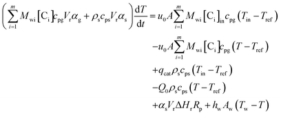
An energy balance based on a pseudo-homogeneous phase is used to predict the temperature of the reactor. In the system, heat is mainly generated from propagation. The unsteady-state energy equation is as follows:

where R_p is the rate of propagation (kmol m⁻³ s⁻¹), A_w the reactor wall area (m²), M_wi the molecular weight of species i, T_w the reactor wall temperature (K), T the reactor temperature (K), c_pg the heat capacity of gas (kJ kg⁻¹ K⁻¹), c_ps the heat capacity of solid (kJ kg⁻¹ K⁻¹), ΔH_r the heat of propagation polymerization (kJ kmol⁻¹), and h_w the heat transfer coefficient between bed to wall (W m⁻² K⁻¹). The bed-to-wall heat transfer coefficient significantly depends on hydrodynamics in the bed.^21–23

The local bed-to-wall heat transfer coefficient was calculated from the following equation:

where T_w is the wall temperature, T_b the bulk temperature, x the distance from the computational node to the heating wall.

The temperature gradient and phase holdups in eqn (5) were calculated in each computational node in the computational domain using CFD model.

The effective thermal conductivity, k_eff, consists of molecular and turbulent thermal conductivities.²⁴ The latter is derived using the analogy between heat and momentum transfer. Therefore, the effective thermal conductivity can be written as:

where k_q is the molecular thermal conductivity for q phase (W m⁻¹ K⁻¹), Pr_t the turbulent Prandtl number.

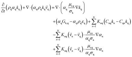
The turbulent viscosity of phase q, μ_t,q, is obtained from solving the conservation of turbulent kinetic energy and turbulent dissipation in CFD hydrodynamic and KTGF models as mentioned in Section 2.4.

2.2 Kinetic rate

The mechanism of propylene polymerization in gas and solid phases is shown in Table 1. It consists of the steps of initiation, propagation, chain transfers, site transformation and deactivation.²⁵ Active catalyst in the solid phase reacts with propylene monomer to form an active monomer. Then, the active monomer reacts repeatedly with propylene to form active dimers and continues to form longer polymer chains. Propagation of active polypropylene with monomer to form longer active polymer chain then proceeds. Finally, the active polymer terminates and becomes a dead polymer chain in either of two mechanisms: chain transfer or termination. The kinetic rate constants for each reaction rate is defined as a function of temperature as Arrhenius' law, with frequency factors and activation energy in terms of a one-site kinetic model, as presented in Table 1.^26–28

Table 1 Polypropylene reaction mechanism and kinetic rate constants

Step of polypropylene polymerization	Reaction	Frequency factor	Activation energy (kcal mol^−1)
(1) Chain initiation		kiM = 1.165 × 10^8 mg^3 kg mol^−1 s^−1	10.5
(2) Chain propagation		kp = 1.370 × 10^9 mg^3 kg mol^−1 s^−1	10.5
(3) Chain transfer
- Transfer to monomer		ktrM = 4.404 × 10^5 mg^3 kg mol^−1 s^−1	10.5
- Transfer to hydrogen		ktrH = 1.528 × 10^7 mg^3 kg mol^−1 s^−1	10.5
(4) Chain termination
- Active polymer deactivation		kd = 9.219 × 10^2 s^−1	10.5
- Catalyst deactivation		kd = 9.219 × 10^2 s^−1	10.5

---

The propagation and deactivation steps are essential steps to define activity of catalysts and productivity. Previously, Zacca and coworkers²⁷ have used a one-site model in good agreement with the experimental data of Drusco and Rinaldi.²⁹ Only small differences between a one-site and a two-site model in terms of overall yield and productivities in polypropylene reactor were found. One site of catalyst was good enough for evaluating the overall yield, productivities and averaged molecular weight, which is our main objective here. Likewise a single lumped model of the reaction rate is adequate for the purpose of this work, giving a reasonable calculation time. The rate constants for this polymerization at 69 °C are obtained from literatures,^27,28 and the activation energy is obtained from Boor.²⁶ The frequency factor and activation energy for this polymerization are shown in Table 1. The reaction rate expressions can be written as shown in eqn (7)–(13) in Table 2.where [C_M] is the concentration of monomer (kmol m⁻³), [C_s,C*] the molar concentration of active catalyst (kmol m⁻³), the molar concentration of active polymer of length i (kmol m⁻³), [C_H2]the concentration of hydrogen (kmol m⁻³), i the degree of polymerization, the molar concentration of active polymer of length 1 or active monomer (kmol m⁻³), and [C_Pi] the molar concentration of dead polymer of length i (kmol m⁻³).

Table 2 Reaction rate expressions for each species

Species	Production rate
Monomer		(7)
Hydrogen		(8)
Active catalyst		(9)
Dead catalyst		(10)
Active chains with length i = 1		(11)
Active chains with length i ≥ 2		(12)
Dead polymer		(13)

---

2.3 Method of moments

A method of moments permits one to solve for moments of chain length distribution with relatively small computational effort. Average chain length can then be easily calculated from the moments and is used for predicting average molecular weight.^5,9,30 Eqn (7)–(13) give the reaction rates based on chain length, which can then be modified into the form of moments by applying the method of moments.^31–33 The zeroth moments of active polymer and dead polymer can be defined as the summation of active and dead polymer, as shown in eqn (14):where λ₀ is the total active polymer, a key parameter determining propagation rate, and μ₀ the total dead polymer. Following this procedure, eqn (7)–(13) are modified in terms of zeroth moment as shown in eqn (15)–(20):

R_M = −k_iM[C_s,C*][C_M] − (k_p + k_trM)[C_M]λ₀ (15)

R_H2 = −k_trH[C_H2]λ₀ (16)

R_C* = −k_iM[C_s,C*][C_M] + k_trM[C_M]λ₀ + k_trH[C_H2]λ₀ − k_d[C_C*] (17)

R_Cs,d = k_dλ₀ + k_d[C_s,C*] (18)

R_λ0 = k_iM[C_s,C*][C_M] − λ₀(k_trM[C_M] + k_trH[C_H2] + k_d) (19)

R_μ0 = λ₀(k_trM[C_M] + k_trH[C_H2] + k_d) (20)

Solving the equations of mass balances, eqn (15)–(20), combined with the kinetic rates in Table 1, the solutions of concentrations of monomer (C_M) and hydrogen (C_H2) in gas phase, concentrations of active (C_s,C*) and dead (C_s,Cd) catalyst can be obtained. In addition, the moments—i.e. zero, first and second moments—of active polymer (λ₀,λ₁,λ₂) and the same of dead polymer (μ₀,μ₁,μ₂) can be calculated using a moment balance:

where R_s,k is the production rate of moments (kmol m⁻³ s⁻¹) and [C_k] the concentration of each moment (kmol m⁻³). Here index k refers to order of moments, while [C_k] refers to λ₀,λ₁,λ₂,μ₀,μ₁,μ₂. The higher moments, (λ₁,λ₂,μ₁,μ₂), are also solved for using the moment conservation equations for predicting molecular weight. The method of moments for first and second moments of active polymer and dead polymer are expressed as follows:

The rate of reaction for higher moments can be written as in eqn (24)–(27):

R_λ1 = k_iM[C_s,C*][C_M] − λ₁ (k_trM[C_M] + k_trH[C_H2] + k_d) + k_p[C_M]λ₀ (24)

R_λ2 = k_iM[C_s,C*][C_M] − λ₂(k_trM[C_M] + k_trH[C_H2] + k_d) + k_p[C_M](2λ₁ + λ₀) (25)

R_μ1 = λ₁(k_trM[C_M] + k_trH[C_H2] + k_d (26)

R_μ2 = λ₂(k_trM[C_M] + k_trH[C_H2] + k_d (27)

Ultimately, using the following equation, the number and weight average molecular weight (M̄_n,M̄_w) are determined:³⁰

2.4 Mathematical model based on CFD

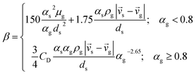
Gas–solid propylene polymerization in a fluidized bed reactor was investigated using a CFD approach for local information prediction. The mathematical models in the overall CFD approach based on conservation for mass, momentum, energy, and species are summarized in Table 3. The interphase momentum transfer coefficient is obtained from Gidaspow's correlations.³⁴ The corresponding shear stress for solid phase is estimated from the kinetic theory of granular flow (KTGF). Granular temperature is proportional to the kinetic energy of the random motion of the particles. The granular temperature transport equations for solid phase is provided by Ding and Gidaspow¹³ as shown in Table 3. Assuming that the granular energy is in steady state and dissipated locally, the convection and diffusion were neglected. Chen³⁵ and coworker has indicated that the results show no significant differences in using this simplification. The granular temperature transport equation can be simplified to an algebraic equation. The closure transport coefficients for solving granular temperature transport equation are listed in Table 4. The Reynold stress related to turbulent viscosity is estimated from the standard k–ε turbulent model. The turbulent kinetic energy, k, and the turbulent dissipation rate, ε, for phase q are obtained by solving eqn (40) and (41) in Table 3. The solutions of turbulent kinetic energy and turbulent dissipation rate of phase q were used to calculate turbulent viscosity aswhere q represents either gas or solid phase and C_μ the turbulent model constant. Further details can be found in the standard k–ε turbulence model proposed by Launder and Spalding.³⁶ The energy balances for gas and solid phases assume that the reactions occur on the solid phase;¹⁵ heat of reaction is thus released to the solid phase. No reaction occurs in the gas phase. The energy balances are written in terms of heat convection and conduction, energy dissipation, heat from species diffusion, heat transfer between phases and heat of polymerization. The interphase heat transfer coefficient between gas and solid is estimated by the Ranz–Marshall equation.³⁷ Polymerization reactor contains gas and solid phases. The gas phase consists of propylene, hydrogen and nitrogen, while the solid phase in the reactor consists of active catalyst, non-active catalyst, dead catalyst and polymer. The species equation can be written in terms of accumulation, convection, diffusion, transfer rate between gas and solid phases and reaction rate.

Table 3 Conservation equations

Equations

Continuity equation for gas and solid phases

(31)

(32)

Momentum balance equations for gas and solid phases

(33)

(34)

Energy balance equations for gas and solid phases

(35)

(36)

Species balance equations for gas and solid phases

(37)

(38)

Granular temperature transport equations for solid phase

(39)

Conservation equation for turbulent kinetic energy

(40)

Conservation equation for turbulent dissipation rate

(41)

---

Table 4 Constitutive equations

Constitutive equations

Solid pressure³⁸

P_s = α_sρ_sθ + 2g₀α_s²ρ_sθ(1 + e)

Radial distribution function³⁹

Solid bulk viscosity³⁹

Solid shear viscosity³⁴

μ_s = μ_s,collision + μ_s,kinetic + μ_s,friction

Diffusion coefficient for granular temperature³⁴

Collisional dissipation of solid fluctuating kinetic energy³⁹

Energy exchange between gas and solid³⁴

ϕ_gs = −3βθ

Interphase momentum transfer coefficient³⁴

Interphase heat transfer coefficient³⁷

Stress tensor

Gas phase

Solid phase

Reynolds stress

---

2.5 Simulation conditions

In this work, a fluidized bed reactor used for polymerization of propylene is continuously fed with propylene, nitrogen and hydrogen at the bottom of the fluidized bed. Hydrogen is a terminator. Solid catalyst particles with a size of 500 microns are also fed continuously at the bottom of the reactor. Polymer product is removed from the bottom of reactor to maintain the level of the bed.

Here a fluidized bed reactor of height 8 m and 2 m in diameter is used in a 2D CFD approach in order to reduce simulation time. The feed and reactor conditions are shown in Table 5. The effects of key process parameters including those of feed catalyst rate, temperature, gas velocity, hydrogen concentration are studied as shown in Table 6.

Table 5 Feed and reactor conditions

	Value
Gas phase
Concentration of each species in feed gas mixture
- Propylene (kmol m^−3)	1.267
- Hydrogen (kmol m^−3)	0.01–0.03
- Nitrogen (kmol m^−3)	0.056
Solid phase
Density, ρs (kg m^−3)	910
Diameter, ds (μm)	500
Mass fraction of each specie in solid catalyst
- Active catalyst	0.008
- Non-active catalyst	0.992
Operating conditions
Pressure, (bar)	25

---

Table 6 Studied effects of operating conditions

Simulation case	u0/umf	Solid loading (kg)	Reactor temperature (K)	Catalyst feed (mg s^−1)	Hydrogen feed concentration (kmol m^−3)
Effect of superficial gas velocity	1.5	2333	330	18.3	0.02
	2.25	3500		27.5
	3	4666		36.7
Effect of feed and wall temperature	2.25	3500	325	27.5	0.02
			330
			335
Effect of catalyst feed	2.25	3500	330	19.2	0.02
				27.5
				35.8
Effect of hydrogen feed concentration	2.25	3500	330	27.5	0.01
					0.02
					0.03

---

2.6 Scaling up

Scale-up of fluidized bed reactors is an attractive challenge. It can be carried out with appropriate criteria so as to obtain similarities in hydrodynamic and reactor performance. The traditional approach focuses on finding scaling laws for various sets of dimensionless numbers.^17,18 Glicksman et al.¹⁷ proposed a set of constant dimensionless parameters obtained by non-dimensionalizing the governing equations of motion for the fluids and the solids in a fluidized bed with expectation to obtain hydrodynamic similarity upon scaling up. Glickman's set of dimensionless numbers are ρ_s/ρ_g, u₀²/gD, u₀/u_mf, G_s/ρ_su₀ and H/D. Nevertheless, scaling up by hydrodynamic similarity is not able to directly predict behavior in a fluidized bed with polymerization. Polymerization does not scale proportionally with increasing reactor size. To maintain polymerization similarity, the weight space time, which is the ratio of the weight of solid particles to the flow rate of monomer, should be fixed in order to have a similar reactor performance. This work studies the effect of scale-up using two different criteria—Set I based on weight space time (τ) similarity and Set II based on H/D similarity—with two different catalyst feed rates.

The scaling relationships and operating conditions of the base case and scaled fluidized beds used for all cases studied are shown in Table 7.

Table 7 Set of dimensionless group for scaling up with different operating conditions and scaling up criteria

	Reactor diameter (m)	ρs/ρg (—)	u0^2/gD × 10^4 (—)	u0/umf (—)	Gs/ρsu0 × 10^5 (—)	H/D (—)	W/FA0 (s)
Set I, 0.044 mg s^−1	0.2	24.4	7.25	2.25	4.10	6.13	251
	2	24.4	7.25	2.25	4.10	1.22	251
	4	24.4	7.25	2.25	4.10	0.87	251
Set I, 0.087 mg s^−1	0.2	24.4	7.25	2.25	8.06	6.13	251
	2	24.4	7.25	2.25	8.06	1.22	251
	4	24.4	7.25	2.25	8.06	0.87	251
Set II, 0.044 mg s^−1	0.2	24.4	7.25	2.25	4.10	6.13	251
	2	24.4	7.25	2.25	4.10	6.13	793
	4	24.4	7.25	2.25	4.10	6.13	1121
Set II, 0.087 mg s^−1	0.2	24.4	7.25	2.25	8.06	6.13	251
	2	24.4	7.25	2.25	8.06	6.13	793
	4	24.4	7.25	2.25	8.06	6.13	1121

---

2.7 Simulation methodology

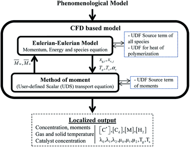
The results from the phenomenological model, with hydrodynamic CFD results of solid fraction and wall heat transfer coefficient, are used as input conditions to solve the Eulerian–Eulerian two-fluid model equations of momentum, continuity, species and energy. To set up the species equations, source terms of gaseous and solid species in terms of complex polymerization rates as a function of moments are included via adding User-Defined Functions (UDF) of source terms. In addition, user-defined equations for transport scalar of each moment (λ₀,λ₁,λ₂,μ₀,μ₁,μ₂), coupled with moments reaction rates, are included. A source term of heat released from polymerization in a UDF form is included in the energy equation. Simulations were carried out in a transient mode. All of the above equations are solved simultaneously via CFD method to provide local mass fraction of each species, phase holdup, phase velocity, phase temperature and active and dead polymer concentrations as seen in Fig. 2. Active and dead polymer concentrations are used for molecular weight calculation. In the present work, all the simulations were carried out in the commercial software ANSYS Fluent 15.0.

Fig. 2 Schematic of coupling CFD with user-defined function.

Inlet velocity, temperature and compositions were specified at the inlet boundary. Pressure with zero gradient conditions of temperature and concentration was defined at the outlet boundary. No slip conditions were specified at the wall for both gas and solid phases. A constant temperature was specified at the wall. The simulation with the time step of 10⁻³ s and a convergence criterion of 10⁻⁵ for each scale residual component with 50 iterations per time step was used.

Grid independency has been checked to ensure that accurate results were obtained. In grid independence studies, the hydrodynamics of systems with three sizes of grid—14,400, 25 600 and 32 400 cells—are simulated. The system with a grid of 25 600 cells offers both good precision and appropriate computational effort and is used to calculate all results.

3. Results and discussion

The results of this work are divided into two main parts: the results based on the phenomenological model and the model based on CFD.

3.1 Results based on phenomenological model

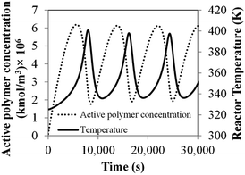
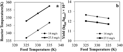
Comprehensive simulated results were obtained to evaluate the effect of the key process parameters—i.e., superficial velocity, feed temperature, catalyst feed rate, hydrogen concentration and reactor size—on production yield, conversion and bed temperature. The results from phenomenological model are as given in the following subsections:

3.1.1 Effect of catalyst feed rate. Typically, catalyst feed rate is increased to obtain higher polymer production rate. To get a picture of the necessary precautions, the catalyst feed rate was varied from 14 to 41.2 mg s⁻¹ holding constant gas feed rate at three different constant feed temperatures so as to show the effects of catalyst feed rate on the reactor temperature and product yield (which the product yield is the production rate per catalyst feed rate). A large reactor size of 2 m diameter, which is on the order of semi-industrial scale, was used. Fig. 3 shows the reactor temperature–time plot for different catalyst feed rates and for various fixed feed temperatures. In the low range of catalyst feed rate (14 to 27.5 mg s⁻¹), the reactor temperature increases with catalyst feed rate. From the start up until 40 000 s, the temperature increases with time and becomes constant. Nevertheless, product yield is not changed significantly with catalyst feed rate. Over the range of higher catalyst feed rate, i.e. 35.8 to 41.2 mg s⁻¹, the reactor temperature fluctuates strongly and can surge up to 400 K. Fig. 3a shows that using the feed temperature of 325 K and the catalyst feed rate of 35.8 mg s⁻¹, the reactor temperature oscillates considerably, over a range of approximately 36 K. With higher catalyst feed rates, 38.5 mg s⁻¹, the reactor temperature overshoot is much higher, and the reactor cannot be operated due to overheating and melting down of the polymer. Then the bed temperature sharply drops from its peak value mainly due to fast active polymer termination arising from high temperature as shown in Fig. 4. The reactor temperature peak lags the active polymer concentration by approximately 2000 seconds. Using the highest catalyst feed rate, 41.2 mg s⁻¹, the bed temperature surges, leading to a runaway condition caused by high active polymer production and its associated high exothermic heat. Fig. 3a–c gives result for different feed temperatures; though exact values differ, for a given catalyst feed rate, reactor temperature follows a similar trend, regardless of feed temperature. However, the amplitude of reactor temperature oscillation is persistently very high for a low feed temperature of 325 K, due to occurring of less catalyst deactivation and active polymer termination, leading to a higher reaction rate and a higher reactor temperature (see Fig. 3a). Such a low-feed temperature condition should be avoided. On the other hand, for higher feed temperatures, less fluctuation of reactor temperature was found due to higher deactivation and termination leading to a lower reaction rate with less heat released (see Fig. 3c); in such a case, the overshooting is minor. Practically, propylene polymerization manufacture is not operated with high range of reactor temperature oscillation because wide range of polymer properties and hotspots has to be avoided. Nevertheless, temperature oscillation behavior upon increasing catalyst flow rate has also found by Ghasem,⁴⁰ Hatzantonis⁷ and Hyanek.⁴¹ Several other papers have also indicated this behavior in polyethylene production. In conclusion, the catalyst feed rate mostly affects the bed temperature. Operating with too high a catalyst feed rate contributes to temperature fluctuation, which leads to overheating and unprofitable catalyst consumption. Using the higher catalyst feed rates (38.5, 41.2 mg s⁻¹), the feed temperature must be increased cautiously so as to moderate both the active catalyst and active polymer concentrations, avoiding overheating, despite these temperature giving higher polymer production rates. The bed temperature is more important to control and focus on than yield in order to improve operability of the polymerization system.

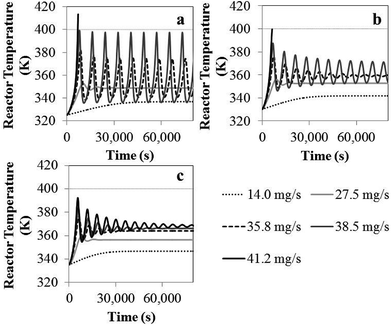Fig. 3 Reactor temperature as a function of time for different catalyst flow rate and feed temperatures: (a) 325 K, (b) 330 K, (c) 335 K.

Fig. 4 Active polymer concentration and reactor temperature as a function of time for feed temperature of 325 K and catalyst flow rate of 38.5 mg s⁻¹.

3.1.2 Effect of feed temperature. The feed temperature was varied from 325 to 335 K, and the wall temperature was set the same as the feed temperature. Results are shown in Fig. 5. In the former, the bed temperature can be seen to increase with the feed temperature for both catalyst flow rate. In the latter, the effect of feed gas temperature on the polymer yield per weight catalyst can be seen. The feed temperature has almost no effect on the polymer yield, which decreases slightly with increasing reactor temperature, as shown in Fig. 5b. This observation was also found experimentally by Wang and coworkers.⁴² In conclusion, the feed temperature mainly affects the reactor temperature. The product yield is not affected significantly by the feed temperature at steady state. Feed temperature adjustment must be of careful concern. Too high a feed temperature should not be used due to an uneconomical product yield.

Fig. 5 (a) Reactor temperature and (b) product yield as a function of feed temperature using a gas superficial velocity of 2.25u_mf and catalyst flow rates of 14 mg s⁻¹ and 27.5 mg s⁻¹.

3.1.3 Effect of superficial gas velocity. The superficial gas velocity, which is a function of gas feed rate in actual operations, affects the hydrodynamics of the system as well as heat and mass transfer. Here it is varied while keeping weight space time constant. Fig. 6 shows the effect of superficial gas velocity on the bed temperature. For low gas velocity (1.5u_mf), the reactor can be easily cooled down due to relatively low solid loading, even though the flow velocity is itself low. At higher gas velocity (2.25u_mf), a proportionally greater solid loading and catalyst feeding are required. The heat removal through the wall at this high loading is not enough—see Fig. 6 for heat transfer coefficients—leading to the highest reactor temperature of all three velocities. However, at the highest gas velocity (3u_mf), considerable movement of solids leads to good mixing and good heat transfer. Thus the bed can be cooled down very well—here one obtains the lowest bed temperature—even though the solid loading is very high. The reactor temperature for the moderate superficial velocity (2.25u_mf) is higher than those for 1.5 and 3u_mf. Using these conditions, the bed temperature oscillated during the initial period of operation. It jumped on the order of 4 °C above the steady state value, leading to undesirable overheating, which is of much concern in commercial operations. Fig. 6 shows the effect of feed velocity on the heat transfer coefficients in the reactor for a constant weight hourly space velocity. Heats of polymerization per mass of product obtained from all cases are similar and on the order of 190 J kg⁻¹ s⁻¹. The heat transfer coefficient increases with gas velocity, as shown in Fig. 6. In conclusion, operation with too low a gas superficial velocity has the disadvantage of poor heat transfer. High feed velocity gives more benefits in terms of heat transfer. Too high a feed velocity has to be avoided because of the entrainment problem.

Fig. 6 Effect of superficial gas velocity at a constant weight hourly space velocity on reactor temperature and heat transfer coefficient.

3.1.4 Effect of hydrogen concentration. Weight average molecular weight of polymer is an important property of any polymerization product. The effect of hydrogen concentration on polymer molecular weight via chain transfer mechanism is studied while keeping constant the other operating conditions. The weight average molecular weight obtained using the hydrogen concentrations of 0.01, 0.02 and 0.03 kmol m⁻³ are approximately 204 000, 167 000 and 141 000, respectively. A higher hydrogen concentration leads to a lower molecular weight because of more chain transfer and thus a shorter chain length. The trend of hydrogen concentration effect on polypropylene molecular weight was also found in Kissin⁴³ and Zhang.⁴⁴

3.1.5 Effect of scale-up. Generally, the purpose of reactor scaling up is to increase the production rate with the same product quality i.e. product yield. Nevertheless, to scale up the fluidized bed reactor with exothermic reaction, the production quality is not only a key parameter to concern. The reactor temperature should be also considered, especially for propylene polymerization reactor. Poor heat transfer may lead to hotspot occurring in the reactor. Consequently, polymer particle can melt and stick together to form bigger particle or fuse into a sheet or chunk resulting in a de-fluidized of particles. Therefore, the objective of this scaling up is to increase production rate with the similarity of product yield and bed temperature. Two different criteria are proposed to scale up fluidized bed reactor. In Set I of polymerization similarity, the weight space time is fixed. In Set II, H/D similarity is required in order to maintain geometric similarity. However, this criterion provides a higher weight space time. A laboratory-scale reactor with a diameter of 0.2 m (m = 1) is scaled up to be a semi-industrial reactor with a diameter of 2 m (m = 10) and finally to a fully industrial-scale reactor with a diameter of 4 m (m = 20). Two base cases are performed with low and high catalyst feed rates, 0.044 and 0.087 mg s⁻¹, respectively. The product yield similarity can be obtained using these two scaled-up parameters as shown in Fig. 7. Nevertheless, two criteria cannot provide reactor temperature similarity as seen in Fig. 8. Obviously, scaling up has more effect on the bed temperature—especially scaling up 10 to 20 times, from a laboratory scale to semi-industrial and industrial scales. Changing from a laboratory to a semi-industrial scale, the bed temperature is hotter. Increasing the reactor diameter from 0.2 m to 2 m, by a factor of 10, the temperature at steady state increases slightly—from 349.4 to 352.7 K for Set I and 351.3 K for Set II. The non-similarity of heat transfer behavior in scaling up has also mentioned in published literature.^45,46

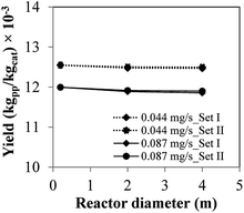Fig. 7 Product yield applying polymerization similarity (Set I) and hydrodynamic similarity (Set II) with catalyst feed rates of 0.044 mg s⁻¹ and 0.087 mg s⁻¹ for the base case (laboratory scale).

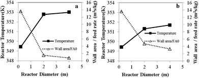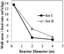
Fig. 8 Effects of reactor scale on reactor temperature and wall area per monomer feed rate for (a) Set I and (b) Set II.

The foregoing differences between heat transfer effects in a small and those in a large reactor depend on the wall area per gas feed rate. As the reactor size increases, the wall surface area per monomer feed rate decreases, resulting in an increase in bed temperature especially in scaling up from 0.2 to 2 m.

In this work, the wall surface area can be obtained using the bed expansion calculated in CFD hydrodynamic simulations. Although the phenomenological model alone cannot provide the bed expansions by itself, in combination with hydrodynamic information from CFD on bed expansion it can provide the wall surface area. Table 8 shows the heat transfer coefficient and wall surface area for different reactor scales following Set I criteria. As the reactor size increases from the laboratory to semi-industrial scale, the heat transfer area per monomer feed rate drops significantly, resulting in an increase in bed temperature. In order to keep the same temperature in scaling up, the heat transfer surface area thus has to be extended. The ways to increase the surface area, such as adding cooling coils, may need to be considered.

Table 8 Heat transfer results for scaling up based on weight space time similarity (Set I)

	Reactor diameter (m)
	0.2	2	4
Volume fraction	0.406	0.369	0.363
Conversion	9.09	9.96	10.01
Reactor temperature, T (K)	349.4	352.8	353.0
Heat transfer coefficient, h (W m^−2 K^−1)	71.30	123.84	164.99
Solid loading (kg)	11	3500	19 799
Bed height at steady state (m)	0.95	3.32	4.77
Reactor heat transfer area, A (m^2)	0.60	20.85	59.99
Heat transfer area/monomer feed rate, A/FA0 (m^2 s kg^−1)	13.57	1.49	0.76
Heat transfer area multiplying factor, f, to keep the same T (349.4 K)	1	4.36	5.26
Adjusted wall temperature to keep same T (349.4 K)	330.15	314.62	312.52

---

Increasing the reactor diameter from 2 to 4 m has less effect on surface area per monomer feed rate than scaling up from 0.2 to 2 m. Table 8 shows that increasing the reactor size to a semi-industrial scale (2 m), the reactor surface area per monomer feed rate is reduced to 1.49 m² s kg⁻¹ in while the bed temperature increases to 352.8 K. In order to maintain the bed temperature of 349.4 K, the desired surface area can be obtained by providing the additional wall surface area. The surface area of the semi-industrial reactor should be increased 4.36 times. That is the surface area of 20.85 m² should be extended to be 90.9 m². To increase the heat transfer area, internal cooling coils or extended surface can be provided. The heat transfer area required to obtain the bed temperature in a semi-industrial scale to match the temperature in a laboratory scale was obtained by trial and error in the full simulation of scaled-up reactors. The required heat transfer area is much larger than available wall surface area with the factor, f, i.e. 4.36. The multiplying factors (f), which can provide the same bed temperatures for all three scales, were obtained and reported in Table 8.

Alternative to extend the wall surface area, the wall temperature can be reduced in order to increase the wall heat removal driving force. The wall temperature for maintaining the same bed temperature was obtained by trial and error of wall temperature in our simulation. In a simulation of scaling up from 0.2 m to 4 m, the wall temperature must be decreased from 330 to 312.5 K to keep a bed temperature of 349.4 K, as shown in Table 8 (the results of other cases are also shown).

Table 9 shows heat transfer parameters in a fluidized bed obtained from Set I scaling-up compared with those from a tubular reactor referred in Nauman,⁴⁵ with the same reaction time throughout. Although the scaling-up from Nauman is for a tubular reactor, it is considered here for comparative discussion. Removal heat from both fluidized bed and tubular reactor is mainly through the wall. In the scaling-up of a tubular reactor with weight space time similarity, the product of heat transfer coefficient and area (hA) can be scaled up by a factor of m^1.7 (see Item 2), as suggested in Nauman.⁴⁵ It was found that increasing from 0.2 m to 4 m, the hA product increased from 43 to 7013 W K⁻¹ for a tubular reactor (Item 2). This can be compared to the simulations in Set I, for which the hA product increases from 43 to 9898 W K⁻¹ (Item 1); note that here the hA product is somewhat higher than that of a tubular reactor.

Table 9 Effect of scaling up on the product of heat transfer coefficient and surface area (hA) in a fluidized bed (using Set I criteria) compared to that in a tubular reactor

	Item	Reactor diameter (m)
		2	4	0.2
	Scaling-up ratio, m	1	10	20
1	hA for fluidized bed with weight space time similarity (W K^−1)	43	2564	9898
2	hA provided for tubular reactor with weight space time similarity = m^1.7 (W K^−1)	43	2159	7013
3	hA suggested for tubular reactor based on heat transfer similarity = m^2.5 (W K^−1)	43	13 620	77 045
4	Adjusted hA (fhA) for fluidized bed with weight space time similarity to maintain the same temperature (W K^−1)	43	11 256	52 061

---

Using weight space time similarity, the reactor temperature cannot be assured constant during scaling up, as indicated in Table 9. Thus, the scaling-up rule based on similarity in heat transfer should be applied. It is suggested that heat transfer similarity in a tubular reactor can be obtained when the hA product has to be scaled up by the factor of m^2.5 (Item 3).⁴⁵ Table 9 shows that as the reactor diameter is increased from 0.2 m to 4 m, the hA product has to be high enough to yield the same bed temperature. It has to be increased from 43 to 77 045 W K⁻¹ in order for a tubular reactor to maintain the reactor temperature of 349.4 K (see Item 3). Referring to this tubular reactor scale-up rule, the hA product in the fluidized bed reactor should be increased in order to maintain the same temperature (see Item 1). In our simulation of a fluidized bed, the heat transfer area multiplying factor, f, has been proposed as shown in Table 8. These multiplying factors are obtained by extensive trial and error in our simulations to keep the same targeted temperature of reactor during the scaling-up process. Table 9 shows that for scaling up from 0.2 to 4 m, the required product of hA for the fluidized bed increases from 43 to 52 061 W K⁻¹ (see Item 4 in Table 9). At 4 m, the hA product of 52 061 W K⁻¹ is required while the hA product of only 9898 W K⁻¹ is available with weight space time similarity (see Item 1). The required hA product is higher (f = 5.26).

The heat transfer parameters in our fluidized bed are of a similar order of magnitude as those in a tubular reactor using the criteria of heat transfer similarity to maintain reactor temperature. They have to be much larger than those obtained from the criteria of weight space time similarity.

Considering reactor scaled up by 20 times based on Set II of hydrodynamic similarity, the criteria yield a slightly lower temperature rise in the order of 1.4 K as shown in Fig. 8. Even though, both criteria give the similar wall heat transfer coefficient, wall surface area from Set II is approximately four times as high as one from Set I. Therefore, heat transfer area multiplying factor for Set II does not require as much as Set I to maintain the same reactor temperature. Moreover, alternative wall temperature reduction for Set II criteria does not need to decrease as low as one from Set I criteria.

In conclusion, to scale up the PP reactor, the overheating of the bed has to be of greater concern than the product yield. Neither criterion (Set I or Set II) can provide heat transfer similarity in scaling up. However, the bed temperature similarity can be achieved by increasing of the wall surface area or decreasing of wall temperature.

3.2 Results based on CFD approach

CFD simulation work was carried out to study the local behavior of reactive flow system. The initializing parameters of the simulation—gas and solid temperatures, gas feed velocity, species concentration, and catalyst concentration—are obtained from the steady-state period of the phenomenological model in order to reduce time required for the full CFD simulation. The simulation results obtained from the model based on CFD can show the local bed temperature variation and other phenomena in the reactor which cannot be provided by the phenomenological model. These simulations can provide information of non-uniformity, overheating and hot spot zones.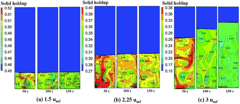

3.2.1 Effect of superficial gas velocity. The superficial velocity of gas, which mainly contains monomer, is varied while keeping constant the solid weight residence time for the sake of keeping the same reaction time for the same feed rate and wall temperature. Thus, the catalyst feed rate is increased proportionally with the monomer feed flow rate as well. Fig. 9 shows the velocity vector plots in a fluidized bed reactor for various feed velocities. Circulation flow of solid particles is found as expected. Fig. 10 shows the contour of solid fraction distribution as well as the isolines indicating quantitative solid fraction at various times of operation for different feed velocities. In starting period of operation before solid movement approaching a steady state, the sold holdup distribution is non-uniform. Bubble behavior can be somewhat captured. However, at a steady state (i.e. 200 s) as the bed fully expended, the solid fraction distribution is rather uniform. The bubble behavior cannot be seen clearly. Many researchers also found bubble behavior in a short time period of operation, i.e. less than 20 s.^35,47 At higher feed velocity, high solid movement and bed expansion lead to lower solid holdup with more uniform distribution. The time-averaged solid volume fraction is 0.489, 0.369 and 0.265 for these three feed velocities.

Fig. 9 Solids velocity vector plots for different superficial gas velocities.

Fig. 10 Contour of solid fraction distribution as well as the isolines indicating quantitative solid fraction at various times of operation for different feed velocities.

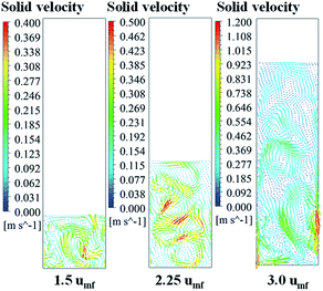
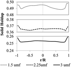
Fig. 11 shows the radial profile of solids holdup averaged between 100 to 200 s for various superficial gas velocities. No significant variation of solid holdup is found with radial position, except near the wall where solid holdup is higher due to the friction between the solid phase and the wall. Similar results have been found in experiments by Wang and co-workers.⁴⁸ At low feed velocity, the radial solid distribution in the bed is relatively non-uniform, while at high feed velocity, more uniformity of solid holdup occurs, as seen in Fig. 11. This characteristic of the radial profile of solid holdup was also found by published literature.^11,49 At low velocity, less bed expansion with high solid holdup was found, leading to less uniformity. On the other hand, at high velocity, high solid movement and bed expansion lead to low solid holdup and more uniformity. The solid holdup can be ranked in order of the cases of 1.5u_mf > 2.25u_mf > 3.0u_mf.

Fig. 11 Radial profiles of solids holdup for different gas superficial velocities.

Fig. 12 shows the contour and radial profiles of monomer concentrations as well as axial profile of monomer conversion for various superficial gas velocities. The monomer decreases slightly with bed height due to monomer being consumed by reaction. However, the conversion of this polymerization is relatively low. Although the flow in the reactor does not behave in a completely well-mixed way (see the vector plot in Fig. 9), the flow has no significant effect on the mass balance.

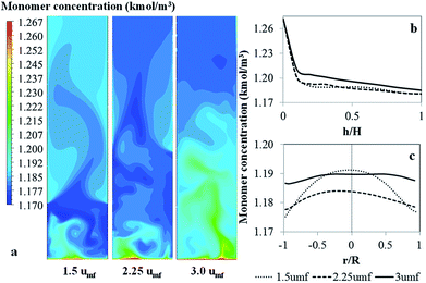Fig. 12 Contour and radial profiles of monomer concentrations as well as axial profile of monomer conversion for various superficial gas velocities.

The assumption of well-mixed flow in the phenomenological model can be applied globally without significant error. However, due to the reaction being highly exothermic, the effect of the flow on the energy balance cannot be ignored. Thus the effects of operating conditions on flow patterns and the local bed temperature are still of significant concern.

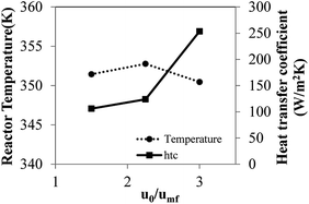
Fig. 13 shows the bed temperature contour plot, and the axial and radial profiles of averaged bed temperature for various superficial gas velocities. The bed temperature is non-uniform due to the reaction being non-isothermal and non-uniformity of flow. The bed is cooler near the cold gas feed zone and rises up along the bed height, but it gradually increases with distance upwards, as shown in Fig. 13b. The temperature difference along the bed height is on the order of 11.1–14.6 K. This axial profile of bed temperature corresponds to the monomer conversion one.

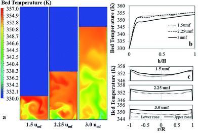Fig. 13 Contour of bed temperature with axial and radial profiles of bed temperature for various superficial gas velocities.

At lower velocity, the radial temperature profile is less uniform. The difference between the maximum and minimum temperatures is 4 K (not including the wall temperature). Compared to the highest velocity (3u_mf), the temperature is lower, and the radial temperature profile is flatter, with a difference between minimum and maximum temperature of 0.87 K. The effect of superficial velocity can be seen in both the radial profile of temperature and the radial profile of monomer concentration, though the effect on one is the opposite of the effect on the other.

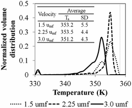
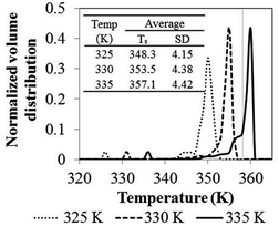
Fig. 14 shows the bed temperature distribution curve in terms of normalized volume distribution. At high feed gas velocity (3u_mf), low mean temperature with less standard deviation (more uniformity of temperature distribution) was found due to high heat transfer and bed expansion. Lower superficial gas velocity creates high solid holdup, leading to higher bed temperature and less uniformity and higher standard deviation than those obtained from high velocity operation. The conversions and product yield change slightly with changes to the superficial gas velocity, as seen in Table 10.

Fig. 14 Bed temperature distribution curves for various superficial gas velocities.

Table 10 Monomer conversion and product yield for all studied effects from CFD

Simulation case	u0/umf	Bed temperature (K)	Catalyst feed rate (mg s^−1)	H2 feed concentration (kmol m^−3)	Conversion (%)	Product yield (kg gcat^−1)
Effect of superficial velocity	1.5	330	27.5	0.02	7.18	12.6
	2.25				7.21	12.7
	3				6.85	12.4
Effect of feed temperature	2.25	325	27.5	0.02	6.85	13.0
		330			7.21	12.7
		335			7.32	12.6
Effect of catalyst feed rate	2.25	330	19.3	0.02	5.32	12.9
			27.5		7.21	12.7
			35.8		9.15	12.4
Effect of hydrogen feed concentration	2.25	330	27.5	0.01	7.22	12.7
				0.02	7.21	12.7
				0.03	7.20	12.6

---

In conclusion, the superficial gas velocity has an effect mainly on the bed temperature and its degree of uniformity with minimal effect on product yield/unit weight of catalyst for the same reaction time, as the system is in a low conversion range. Higher superficial velocity gives more uniformity of bed temperature.

3.2.2 Effect of feed temperature. The feed temperature was varied: 325, 330 and 335 K. Fig. 15 shows the contour of monomer concentration and bed temperature in the bed at various feed temperatures. At the lowest feed temperature (325 K), less monomer is consumed since there is a lower reaction rate, which produces less heat and results in lower bed temperature and more uniformity of the monomer concentration distribution, compared with those at higher feed temperatures (330 and 335 K), as seen in Fig. 15b, the contour of bed temperature, and Fig. 16, the average bed temperatures and their standard deviation. In the cases of 325 and 330 K, no hot spot zone was found. A average bed temperature of 353 K is usually the accepted industrial safety limit.⁵⁰ Thus a hot spot zone in this work is defined as a place where the local bed temperature is above 358 K. Operating above this critical temperature may lead to sticky particle agglomeration in the reactor, leading to de-fluidization operation. At the high feed temperature (335 K), the average bed temperature (357.1 K) is at the acceptable limit, but the hot spot zones constitute 62% of the volume and should be seriously accounted for (see Fig. 16). At this high feed temperature (335 K), the phenomenological model shows a bed temperature of 356 K with no overheating. The CFD simulation provides a bed temperature in a range of 335 to 359.7 K with an overheating zone of 62% by bed volume. The averaged value is 357.1 K which deviates on a little from the value of 356 K obtained in the phenomenological model. The effect of feed temperature on conversion and product yield is also shown in Table 10. It can be seen that the feed temperature has only a small effect on monomer conversion and yield. In conclusion, the uniformity of bed temperature increases with decreasing gas feed temperature. Moreover, operating with too high a temperature reveals a high possibility of hotspots and non-uniformity of bed temperature.

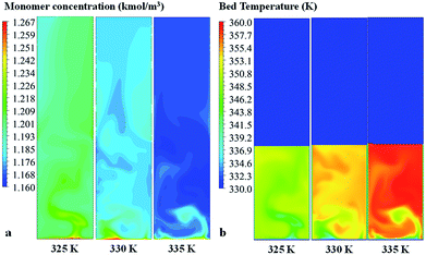Fig. 15 Contour of (a) propylene concentration and (b) bed temperature in the fluidized bed for various feed temperatures.

Fig. 16 Bed temperature distribution for various feed temperatures.

3.2.3 Effect of catalyst feed rate. The effect of catalyst feed rate was studied by varying catalyst feed rate from 19.2 to 35.8 mg s⁻¹. The gas feed flow rate and operation temperature were kept constant. Fig. 17 shows the contours of propylene concentration and bed temperature. With increasing catalyst feed rate, the conversion increases due to there being more available catalyst in the reactor, leading to monomer concentration decreased and thus a high heat of polymerization released (causing higher bed temperature). The hotspots constitute found to be 85% by volume of the bed with a high mean temperature of 359.2 K and more non-uniformity and higher standard deviation of temperature (see Fig. 18). This leads to operation problems as previously mentioned.

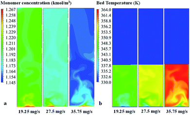Fig. 17 Contours of (a) propylene concentration and (b) bed temperature in the fluidized bed for various catalyst feed rates.

Fig. 18 Bed temperature distribution curves for various catalyst feed rates.

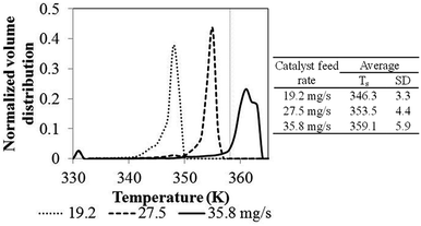
Comparing to phenomenological model, at this high catalyst feed rate (35.8 mg s⁻¹), both results show that the system cannot be operated at the limit temperature wise (358 K), whereas the CFD based model shows a significant problem of hotspots. At the low feed catalyst rates of 19.2 and 27.5 mg s⁻¹, the problem in overheating was not found. In conclusion, the non-uniformity of bed temperature and overheating in the bed has to be of concern when increasing the catalyst flow rate for improving production.

3.2.4 Effect of hydrogen concentration. The effect of hydrogen feed concentration was studied by varying hydrogen concentrations in the feed from 0.01 to 0.03 kmol m⁻³ to control the molecular weight of the product.

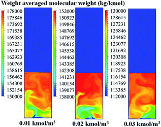
To study its effect on the local distribution of the weight average molecular weight, CFD calculation was carried out from the beginning to 100 seconds of operation. Fig. 19 shows that the weight average molecular weight increases with decreasing hydrogen concentration, due to lower chain transfer to hydrogen. The molecular weight is clearly non-uniform and increases significantly with position along the bed height for all cases studied. Short chain polymer was found near the bed bottom because more fresh catalyst and hydrogen are found near the feed area. On the other hand, longer polymer chain was found near the top of the bed due to a longer residence time with less transfer and termination. The finding is beneficial for positioning product withdrawal outlet.

Fig. 19 Contour of weight average molecular weight in the fluidized bed for various hydrogen feed concentrations at 100 s.

3.2.5 Effect of scale up. Scale-up of fluidized bed reactors is a challenge in chemical reaction engineering, especially when it pertains to a polymerization reactor. From the study on the effect of scaling-up based on the phenomenological model in the Section 3.1.5, product yield does not change with reactor size. Nevertheless, the similarity of heat transfer cannot be simply obtained. For more clear understanding on the heat transfer, this section shows the effect of scaling-up on the distribution of bed temperature for two separate criteria: Set I based on solid weight time (τ) constant and Set II based on Glickman's H/D constant.

Fig. 20a and b show the solid holdup contours for different sizes of fluidized bed reactors using weight time (Set I) and H/D (Set II) constants, respectively. Fig. 20a shows that the ratio of fluidized bed height to bed diameter (H_expand/D) decreases as the reactor is scaled up for Set I (resulting from decreasing of the ratio of initial bed height to diameter (H_ini/D) as the reactor size increases). In spite of there being a lower bed height at the industrial scale, the solid holdup is also lower, as shown in Fig. 20a. Fig. 20b shows the effect of scaling up on the solid holdup based on Set II criteria. H/D constant was carried out by keeping the same ratio of initial solid bed height to reactor diameter (H_ini/D), in expectation that the same ratio of fluidized bed height to diameter (H_expand/D) would also ensure. The results show that the hydrodynamics are not similar for these three scales. As the reactor diameter is increased from 0.2 to 4 m, H_expand/D increases from 4.7 to 5.4 and the solid holdup decreases from 0.41 to 0.36 at the same ratio of u₀/u_mf. Neither criterion provides similar hydrodynamic results. Thus similarity in heat and mass transfer in scaling up is not obtained. One can adjust the superficial gas velocity or particle size to obtain the same solid holdup. Even though, the same solid holdup is obtained, the same heat transfer in the bed cannot be ensured.

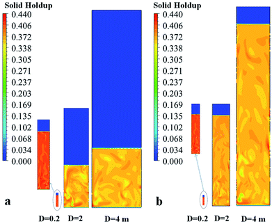Fig. 20 Contours of solid holdup for different reactor scales for (a) Set I with weight space time similarity, and (b) Set II with hydrodynamic similarity.

Fig. 21 and 22 show the contour and radial profiles of bed temperature for different reactor sizes and scaling criteria. For the semi-industrial and industrial scale reactors (D = 2, 4 m, respectively), the magnitudes of bed temperature in Fig. 22 are not much different.

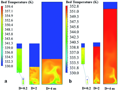Fig. 21 Contour of bed temperature for different reactor scales obtained using (a) Set I with weight space time similarity, and (b) Set II with hydrodynamic similarity.

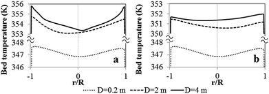Fig. 22 Radial profiles of bed temperature for different reactor scales for (a) Set I and (b) Set II criteria.

In the laboratory reactor scale, the bed temperature is lower and its radial profile is flatter than those of the semi-industrial and industrial reactors due to better heat removal at the smaller scale. It should be noted that, although the solid holdup obtained in the largest scale is lower, the temperature is higher. Scaling up the reactor from the laboratory scale to industrial scale, the temperature increases due to lower wall heat transfer area per unit of feed rate, as seen in Fig. 23. The ratio decreases with rector size.

Fig. 23 Effect of reactor scales on wall area per monomer feed rate for Set I and Set II criteria.

Fig. 24 shows the temperature distribution for various reactor scales calculated using weight time similarity (Set I) criteria. The standard deviation of temperature in the reactor is in the range of 2.9–4.5 K and increases with reactor scale, as shown in Fig. 24. This trend was also found in the results of phenomenological model shown in Section 3.1.5. It confirms that more non-uniformity of bed temperature occurs in a larger scale reactor. In conclusion, neither scaling-up criterion can provide uniformity and similarity of temperature in reactor. Scaling up using Set II criteria provides more uniformity of temperature due to the advantage of higher ratio of wall surface area to monomer feed rate.

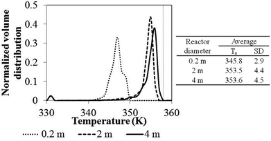Fig. 24 Bed temperature distribution for different reactor scales using weight time similarity (Set I) criteria.

In all, the results based on the CFD approach coupled with phenomenological model gives a new insight of the heat effect and temperature distributions in fluidized bed for propylene polymerization. A better operation, design, and scale up of reactor should be realized.

3.3 Comparison of the results from the phenomenological model and available results in literature

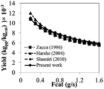
The operating information of polyolefin industrial systems is proprietary and extremely hard to find. Therefore, the results of the phenomenological model used here are compared to previously published simulation work. Fig. 25 shows the comparison in terms of product yield based on the effect of catalyst feed rate for an isothermal operation. A list of simulation parameters used for comparison is shown in Table 11. It can be observed that the product yield predicted from this current model agrees well with the previously published work of Harshe,⁶ Shamiri⁹ and Zacca.²⁷ Polymer properties are basically defined by molecular weight. The mass averaged molecular weight at steady state calculated from this current model compares satisfactory to the work of Shamiri, as they give values of 166 700 and 163 200, respectively. The percent difference is 2.12%. Moreover the calculated results from this model were validated with the previous experimental data obtained by Shamiri.⁵¹ The experiments were carried out in a fluidized bed of 0.1016 m in diameter, feed temperature of 333 K and catalyst flow rate of 3.02 g h⁻¹. The time plots of propylene concentration and reactor temperature obtained from the phenomenological model and the experiments at the same conditions were compared as shown in Fig. 26. It can be observed that the results of this current model show a satisfactory level of agreement with the experimental results of Shamiri.⁵¹ The phenomenological model is applicable and comparable with previous work in terms of product yield and molecular weight. However, from this work, additional information of heat transfer effect is available especially in scaling-up. Detailed information of heat effects in a polymerization fluidized bed reactor obtained from this work is an insight which will be useful for reactor operation, analysis, designs and scaling-up improvement.

Fig. 25 Comparison of results from the phenomenological model with previously published works.

Table 11 Operating conditions and physical parameters used for comparing with previously published work

Operating conditions and physical parameters

T_r (K) = 343.15 V_r (m³) = 50

P (bar) = 25 u₀ (m s⁻¹) = 0.35

Propylene concentration (kmol m⁻³) = 1.267

Hydrogen concentration (kmol m⁻³) = 0.02

Weight fraction of titanium in catalyst = 0.4

Fraction of active titanium = 2%

ρ_s (kg m⁻³) = 910 d_p (micron) = 500

---

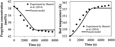Fig. 26 Comparison between experimental data and calculated results of propylene concentration and reactor temperature.

3.4 Practical significance and limitation of the models

The combined model consisting of phenomenological model and CFD-based reactor model can predict various level scales of reactor performance. The former model can provide overall information while the latter can provide local information. The average results suggest improved productivity and reactor temperature control done by cautiously adjusting the operating conditions e.g. increasing catalyst feed rate, operating temperature, reactor size and superficial velocity, with consideration of catalyst deactivation. Improper conditions for increasing productivity can involve a risk with regards to control of oscillating temperature. The model identifies an operating window to improve productivity and temperature control and to study operation details. The local information obtained from the CFD-based reactor model is useful to find the region of hotspots by evaluating the temperature distribution in the reactor. Both models provides information for the selection of the proper operating conditions and safe range of operation. They are useful for analysis of a laboratory reactor and an industrial scale reactor and provide information on scale up. Hydrodynamic and heat transfer similarities in different reactor scales, which can be predicted by this model, are useful for scaling up.

Upon scaling up, the finding shows that heat transfer area is critical for design and need a careful consideration by either increasing the area to satisfy the requirement or increasing temperature driving force by reduction of wall temperature, especially in large scale reactor. CFD spends a large of computational time. If only global information is needed, the phenomenological model is sufficiently applied. The combined model cannot provide details of molecular weight distribution unless more detailed kinetic rates are used. However, with the limitation in term of large computational time, the CFD based model is impractical. Only the phenomenological model can be used. The CFD-based model is based on two-fluid model which assumes a continuum phase of solid particles. Therefore, this model can be applied for different modes of fluidized bed with a small particle size, but not for the one with a large particle size. For instance, a fluidized bed with a spouted mode of operation cannot be studied accurately by this model. Other models, e.g. Lagrangian model, should be used instead.

4. Summary

This work has presented a detailed performance model of propylene polymerization in a continuous fluidized bed reactor, using both a phenomenological model and CFD combined with the method of moment. The phenomenological model provides average bed temperature, monomer concentration, polymer production rate and molecular weight in polymerization reactor. Meanwhile, CFD-based reactor analysis provides distributions of phase movements and temperature. The effects of operating conditions and scaling up on the reactor temperature control were focused on. Based on the results of these two approaches, suggestions can be drawn for improving productivity and reactor temperature control include cautiously increasing catalyst feed rate, operating temperature, hydrogen concentration, reactor size and superficial velocity. The details and highlight of key results are as follows.

• In general, high catalyst loading is beneficial only up to a certain point, beyond which the phenomenological model showed that a sustained oscillation of productivity and reactor temperature occurs.

• The benefits of increasing productivity by increasing catalyst feed rate should be balanced with consideration of hotspots occurrence and control of oscillating temperature. Additionally, the reactor temperature and production yield need to be balanced with consideration of a risk of the hotspot formation.

• Increasing operating temperature does not always increase production rate because of catalyst deactivation. Reactor performance can be identified by the simple well-mixed model to improve productivity and study operation details.

• Propylene conversions from both CFD and the phenomenological model show that the mixing effect is not very significant excepting in hotspot generation.

• Superficial gas velocity strongly affects the fluidized regime and heat transfer. Scaling up using two different criteria—Set I based on weight space time (τ) similarity and Set II based on H/D similarity—can not provide heat transfer similarity.

• In scaling up the PP fluidized bed, the operating temperature in the reactor should be chosen while taking into account the ratio of internal wall area to monomer feed rate and the temperature difference between bulk and wall, as well as hydrodynamic behavior in the reactor.

• To keep the same reactor temperature in scaling up a reactor from 0.2 to 4 m in diameter requires a heat transfer area multiplying factor of 2.43 to 5.26 or lowering the wall temperature in the range of 7 to 18 K.

• The CFD model is therefore more useful than the phenomenological model to find the region of hotspots, as it works by evaluating the temperature distribution in each section of fluidized bed reactor.

• Temperature variations in the range of 10 to 14 K were observed in the top section of the reactor in the CFD model and fall within an acceptable operating window. However, when the operating conditions are changed, CFD should be applied to check again for the possibility of local hotspots.

Both models provide useful information for the selection of appropriate operating conditions and a safe range of operation windows. They are useful for analysis of both laboratory reactors and industrial-scale reactors and provide information on scaling up.

Conflicts of interest

There are no conflicts to declare.

Notation

A	Cross sectional area of fluidized bed reactor, (m^2)
Aw	Reactor wall area, (m^2)
[Ci]	Molar concentration of species i in the gas phase, (kmol m^−3)
[Cs,j]	Molar concentration of species j in the solid phase, (kmol m^−3)
[Ck]	Molar concentration of moments k in solid phase, (kmol m^−3)
CD	Drag function
cpq	Heat capacity of phase q, (kJ kg^−1 K^−1)
ds	Particle diameter, (m)
e	Restitution coefficient between particle
FA0	Monomer flow rate, (kg s^−1)
g0	Radial distribution function
Gs	Solids mass flux, (kg m^−2 s^−1)
Gk,q	Production of turbulent kinetic energy of phase q, (kg m s^−3)
hg	Specific enthalpy of gas phase, (kJ kg^−1)
ΔHr	Heat of propylene polymerization, (kJ kmol^−1)
H	Bed height, (m)
hgs	Heat transfer coefficient between gas and solid, (W m^−2 K^−1)
hw	Wall heat transfer coefficient, (Wm^−2 K^−1)
I	Unit tensor
J⃑g,i	The diffusion flux of gas phase for species i, (kg m^−2 s^−1)
kq	Turbulent kinetic energy of phase q, (m^2 s^−2)
kiM	Frequency factors for initiation, (m^3 kmol^−1 s^−1)
kp	Frequency factors for propagation, (m^3 kmol^−1 s^−1)
ktrM	Frequency factors for chain transfer to monomer, (m^3 kmol^−1 s^−1)
ktrH	Frequency factors for chain transfer to hydrogen, (m^3 kmol^−1 s^−1)
kd	Frequency factors for chain termination, (1/s)
keff,q	Effective thermal conductivity of phase q, (W m^−1 K^−1)
kθs	Diffusion coefficient for granular temperature, (kg m^−1 s^−1)
Knq	Turbulent interphase momentum transfer coefficient between phase n and phase q, (kg m^−3 s^−1)
m	Diameter scale ratio
ṁgs	Mass transfer rate between gas and solid phases, (kg m^−3 s^−1)
M̄n	Number average molecular weight, (kg kmol^−1)
M̄w	Weight average molecular weight, (kg kmol^−1)
Mwi	Molecular weight of species i, (kg kmol^−1)
P	Pressure, (Pa)
Ps	Solids pressure, (Pa)
q⃑g	Heat flux from species diffusion, (W m^−2)
qcat	Volumetric flow rate of catalyst feeding, (m^3 s^−1)
Q0	Volumetric flow rate of polymer removal, (m^3 s^−1)
Q	Heat transfer from the bed to wall, (W m^−3)
Rp	Rate of propagation, (kmol m^−3 s^−1)
Rg,i	Production rate of species i from gas to solid, (kmol m^−3 s^−1)
Rs,j	Production rate of species j in solid phase, (kmol m^−3 s^−1)
Rs,k	Production rate of moments k in solid phase, (kmol m^−3 s^−1)
Ss	Heat production of reaction on solid phase, (kJ m^−3 s^−1)
T	Reactor temperature, (K)
Tq	Temperature of phase q, (K)
Tw	Wall temperature, (K)
u0	Superficial velocity of gas, (m s^−1)
umf	Minimum fluidized velocity, (m s^−1)
v⃑q	Velocity of phase q, (m s^−1)
Vr	Reactor volume, (m^3)
W	Solid loading, (kg)
WTi	Weight fraction of titanium in the catalyst
xq,i	Mass fraction of i species in phase q
XTi	Fraction of titanium atoms that are catalyst sites
x	The distance from the computational node to the heating wall, (m)
MwM	Molecular weight of monomer (kg kmol^−1)

Greek letters

αi	Volume fraction of i phase
β	Inter phase momentum transfer coefficient from gas to solid, (kg m^−3 s^−1)
ξs	Solid bulk viscosity, (Pa s)
εq	Turbulent dissipation rate of phase q (m^2 s^−3)
λi	Molar concentration of ith moment for active polymer on solid, (kmol m^−3); i = 0, 1, 2
μi	Molar concentration of ith moment for dead polymer on solid, (kmol m^−3); i = 0, 1, 2
μq	Viscosity of phase q, (Pa s)
μt,q	Turbulent viscosity of phase q, (Pa s)
θ	Granular temperature, (m^2 s^−2)
	Shear stress tensor, (N m^−2)
	Reynolds stress tensor, (N m^−2)
γθs	Collisional dissipation of solid fluctuating kinetic energy, (kg m^−1 s^−3)
ϕgs	Energy exchange between gas and solid, (kg m^−1 s^−3)
σε	Turbulent Prandtl number for the dissipation rate
σk	Turbulent Prandtl number for the turbulent kinetic energy

Subscriptions

g	Gas phase
s	Solid phase
t	Turbulent

Acknowledgements

This work was financially supported by the Kasetsart University Research and Development Institute (KURDI), the Faculty of Engineering of Kasetsart University, the Centre of Excellence on Petrochemical and Materials Technology (PETROMAT) and the Centre for Advanced Studies in Industrial Technology.

References

1. R. Fan, PhD thesis, Iowa State University, Iowa, 2006.
2. A. Ahmadzadeh, H. Arastoopour, F. Teymour and M. Strumendo, Chem. Eng. Res. Des., 2008, 86, 329–343.
3. J. Y. Kim and K. Y. Choi, Chem. Eng. Sci., 2001, 56, 4069–4083.
4. K. B. McAuley, J. F. MacGregor and A. E. Hamielec, AIChE J., 1990, 36, 837–850.
5. K. B. McAuley, J. P. Talbot and T. J. Harris, Chem. Eng. Sci., 1994, 49, 2035–2045.
6. Y. M. Harshe, R. P. Utikar and V. V. Ranade, Chem. Eng. Sci., 2004, 59, 5145–5156.
7. H. Hatzantonis, H. Yiannoulakis, A. Yiagopoulos and C. Kiparissides, Chem. Eng. Sci., 2000, 55, 3237–3259.
8. A. Shamiri, M. A. Hussain, F. S. Mjalli and N. Mostoufi, Comput. Chem. Eng., 2012, 36, 35–47.
9. A. Shamiri, M. A. Hussain, F. S. Mjalli and N. Mostoufi, Chem. Eng. J., 2010, 161, 240–249.
10. A. Shamiri, S. W. Wong, M. F. Zanil, M. A. Hussain and N. Mostoufi, Chem. Eng. J., 2015, 264, 706–719.
11. S. Benzarti, H. Mhiri and H. Bournot, World Acad. Sci. Eng. Technol., 2012, 6, 111–116.
12. P. Khongprom, A. Aimdilokwong, S. Limtrakul, T. Vatanatham and P. A. Ramachandran, Chem. Eng. Sci., 2012, 73, 8–19.
13. J. Ding and D. Gidaspow, AIChE J., 1990, 36, 523–538.
14. M. Xu, F. Chen, X. Liu, W. Ge and J. Li, Chem. Eng. J., 2012, 207–208, 746–757.
15. Y. Yao, Y. J. He, Z. H. Luo and L. Shi, Adv. Powder Technol., 2014, 25, 1474–1482.
16. Z. Li, M. van Sint Annaland, J. A. M. Kuipers and N. G. Deen, Chem. Eng. Sci., 2016, 140, 279–290.
17. L. R. Glicksman, M. R. Hyre and P. A. Farrell, Int. J. Multiphase Flow, 1994, 20, 331–386.
18. L. R. Glicksman, M. Hyre and K. Woloshun, Powder Technol., 1993, 77, 177–199.
19. D. Kunii and O. Levenspiel, Fluidization engineering, Butterworth-Heinmann, Boston, MA, 2nd edn, 1991.
20. H. Cui, N. Mostoufi and J. Chaouki, Chem. Eng. J., 2000, 79, 133–143.
21. J. C. Chen, J. R. Grace and M. R. Golriz, Powder Technol., 2005, 150, 123–132.
22. P. Basu, Combustion and Gasification in Fluidized Beds, CRC Press, 2006.
23. A. Blaszczuk, W. Nowak and J. Krzywanski, Powder Technol., 2017, 316, 111–122.
24. ANSYS, FLUENT Theory Guide, Northbrook, IL, 2009.
25. Y. P. Zhu, Z. H. Luo and J. Xiao, Comput. Chem. Eng., 2014, 71, 39–51.
26. J. Boor, Ziegler-Natta Catalysts Polymerizations, Academic Press, New York, 1st edn, 1979.
27. J. J. Zacca, J. A. Debling and W. H. Ray, Chem. Eng. Sci., 1996, 51, 4859–4886.
28. Z. H. Luo, P. L. Su, D. P. Shi and Z. W. Zheng, Chem. Eng. J., 2009, 149, 370–382.
29. G. Di Drusco and R. Rinaldi, Hydrocarbon Process., 1984, 55, 113–117.
30. J. B. P. Soares, Chem. Eng. Sci., 2001, 56, 4131–4153.
31. S. Zhu, J. Polym. Sci., Part B: Polym. Phys., 1999, 37, 2692–2704.
32. W. Zhou, E. Marshall and L. Oshinowo, Ind. Eng. Chem. Res., 2001, 40, 5533–5542.
33. R. Wang, Y. Luo, B. Li, X. Sun and S. Zhu, Macromol. Theory Simul., 2006, 15, 356–368.
34. D. Gidaspow, R. Bezburuah and J. Ding, Proc. Seventh Eng. Foundation Conf. Fluid.
35. X. Z. Chen, D. P. Shi, X. Gao and Z. H. Luo, Powder Technol., 2011, 205, 276–288.
36. B. E. Launder and D. B. Spalding, Comput. Methods Appl. Mech. Eng., 1974, 3, 269–289.
37. W. E. Ranz and W. R. Marshall, Chem. Eng. Prog., 1952, 48, 141–146.
38. M. Syamlal, W. Rogers and T. J. O'Brien, MFIX documentation theory guide, 1993.
39. C. K. K. Lun, S. B. Savage, D. J. Jeffrey and N. Chepurniy, J. Fluid Mech., 1984, 140, 223–256.
40. N. M. Ghasem, W. L. Ang and M. A. Hussain, Korean J. Chem. Eng., 2009, 26, 603–611.
41. I. Hyanek, J. Zacca, F. Teymour and W. H. Ray, Ind. Eng. Chem. Res., 1995, 34, 3872–3877.
42. Q. Wang, Y. Lin, Z. Zhang, B. Liu and M. Terano, J. Appl. Polym. Sci., 2006, 100, 1978–1982.
43. Y. V. Kissin, L. A. Rishina and E. I. Vizen, J. Polym. Sci., Part A: Polym. Chem., 2002, 40, 1899–1911.
44. H. X. Zhang, Y. J. Lee, J. R. Park, D. H. Lee and K. B. Yoon, Polym. Bull., 2011, 67, 1519–1527.
45. E. B. Nauman, Chemical Reactor Design, Optimization, and Scaleup, John Wiley & Sons, Inc., Hoboken, New Jersey, New York, 2008.
46. G. Wu, Q. Wang, K. Zhang and X. Wu, Powder Technol., 2016, 304, 120–133.
47. L. Wang, X. Xie, G. Wei and R. Li, Part. Sci. Technol., 2017, 35, 177–182.
48. Z. Wang, D. Bai and Y. Jin, Powder Technol., 1992, 70, 271–275.
49. R. Gujjula and N. Mangadoddy, Part. Sci. Technol., 2015, 33, 593–609.
50. G. B. Meier, G. Weickert and W. P. M. Van Swaaij, J. Polym. Sci., Part A: Polym. Chem., 2001, 39, 500–513.
51. A. Shamiri, M. A. Hussain, F. S. Mjalli, M. S. Shafeeyan and N. Mostoufi, Ind. Eng. Chem. Res., 2014, 53, 8694–8705.

---