
 Open Access Article
 This Open Access Article is licensed under a Creative Commons Attribution-Non Commercial 3.0 Unported Licence
A novel adaptive ensemble classification framework for ADME prediction†
Ming Yang ab,
Jialei Chena,
Liwen Xua,
Xiufeng Shia,
Xin Zhoua,
Zhijun Xia,
Rui An*b and
Xinhong Wang*b
ab,
Jialei Chena,
Liwen Xua,
Xiufeng Shia,
Xin Zhoua,
Zhijun Xia,
Rui An*b and
Xinhong Wang*b
aDepartment of Pharmacy, Longhua Hospital Affiliated to Shanghai University of TCM, Shanghai, People's Republic of China
bDepartment of Chemistry, College of Pharmacy, Shanghai University of Traditional Chinese Medicine, Shanghai, People's Republic of China. E-mail: wxh6020@163.com; anruimw@126.com
First published on 26th March 2018
Abstract
It has now become clear that in silico prediction of ADME (absorption, distribution, metabolism, and elimination) characteristics is an important component of the drug discovery process. Therefore, there has been considerable interest in the development of in silico modeling of ADME prediction in recent years. Despite the advances in this field, there remains challenges when facing the unbalanced and high dimensionality problems simultaneously. In this work, we introduce a novel adaptive ensemble classification framework named as AECF to deal with the above issues. AECF includes four components which are (1) data balancing, (2) generating individual models, (3) combining individual models, and (4) optimizing the ensemble. We considered five sampling methods, seven base modeling techniques, and ten ensemble rules to build a choice pool. The proper route of constructing predictive models was determined automatically according to the imbalance ratio (IR). With the adaptive characteristics of AECF, it can be used to work on the different kinds of ADME data, and the balanced data is a special case in AECF. We evaluated the performance of our approach using five extensive ADME datasets concerning Caco-2 cell permeability (CacoP), human intestinal absorption (HIA), oral bioavailability (OB), and P-glycoprotein (P-gp) binders (substrates/inhibitors, PS/PI). The performance of AECF was evaluated on two independent datasets, and the average AUC values were 0.8574–0.8602, 0.8968–0.9182, 0.7821–0.7981, 0.8139–0.8311, and 0.8874–0.8898 for CacoP, HIA, OB, PS and PI, respectively. Our results show that AECF can provide better performance and generality compared with individual models and two representative ensemble methods bagging and boosting. Furthermore, the degree of complementarity among the AECF ensemble members was investigated for the purpose of elucidating the potential advantages of our framework. We found that AECF can effectively select complementary members to construct predictive models by our auto-adaptive optimization approach, and the additional diversity in both sample and feature space mainly contribute to the complementarity of ensemble members.
Introduction
Nowadays, it is important to introduce early absorption, distribution, metabolism and excretion (ADME) profiling in parallel with optimization of efficacy in drug discovery. The poor ADME properties are largely accountable for drug failure in the late-stage development phase. The early ADME profiling approaches allow for the prioritization of drug candidates over their biopharmaceutical properties. With the advances in combinatorial chemistry and high-throughput techniques, large libraries of chemicals are available, and can be screened at higher throughput. In silico modeling, as compared to the traditional in vitro/vivo test, is lower-cost and time-saving. Over the past few decades, more robust models have been established to predict various ADME properties, including membrane permeability,1,2 intestinal absorption (IA),3,4 oral bioavailability (OB),5–7 human ether-a-go-go related gene binders,8–10 as well as transporter binders.11,12 Most of these models were based on quantitative-structure active relationship (QSAR) approach, ranging from simple multiple linear regression to complex machine learning techniques, such as partial least squares discriminant analysis (PLSDA),13 naive bayes (NB) classifier,10,14 Kohonen self-organizing maps,15 k nearest neighbor (KNN),5,16,17 artificial neural networks (NNET),18 support vector machine (SVM),5,16,17,19 and random forest (RF).5,16,17 However, there remain some challenges when developing these methods. First, unbalanced situations often occurs in ADME data due to the publications biased to the favorable property. It refers to datasets in which samples from some classes greatly outnumber samples from others.20 For the binary ADME classification, the number of unfavorable compounds is much less than favorable ones. Such skewed class distribution has detrimental effects on the performance of conventional classifiers which are driven by accuracy. Several studies balanced data sets by changing the classification cutoff. For instance, Xue et al.21 used 70% as threshold to classify the good IA and poor IA, and 80% was used to differentiate the good OB and the poor OB.22 However, these cutoff values may be unreasonable in practice,23 consequently limiting the application of these predictive models in drug design. In addition, a large number of molecular descriptors were calculated to quantitatively define structural and physicochemical properties when modeling. This high dimensionality makes unbalanced classification hard.24 The samples of minority class tends to be sparse as dimensionality increasing, leading to amplifying the issue of skewed class distribution.25 Some studies24,26–28 reported that the classification performance heavily degenerated when using conventional classifiers for high-dimensional and unbalanced datasets.In order to address the unbalanced problem, a number of techniques can be carried out. These methods can be divided into two main categories: the data level and the algorithm level.20 The data level methods, also named sampling methods, preprocess the training data to make them balanced by increasing the minority class compounds, eliminating the majority class compounds, or the hybrid strategy. Some of the most popular ones are such as oversampling and undersampling. Sampling methods were effective in solving the class unbalanced problem. However, the benefits of these preprocess techniques may vary in characteristics of datasets.20,29 Furthermore, some potential useful data may be omitted when modeling on a very small balanced subset from the original data by some methods such as the undersampling based approaches.30 The algorithm level methods reduce the sensitiveness to class unbalance by modifications of existing classification algorithms. These cost-sensitive methods including the modified SVM,19 RF,31 and classification and regression tree (CART)32 were successfully used to handle the unbalanced problem of predicting IA. Recently, Hai's study33 showed that sampling based methods displayed better performance than the cost-sensitive methods for Caco-2 cell permeability (CacoP) prediction. Moreover, it is not easy to achieve the accurate misclassification cost when applying the cost-sensitive methods.30 Some recent work29,30 found that both the data level and the algorithm level were problem dependent, and the selection of proper strategy was largely based on data characteristics.
Ensemble methods have gained popularity in recent years, and they have been used to handle the unbalanced problem in many studies.34–37 The general idea of ensemble methods lies in the aggregation from several individual models in an attempt to obtain substantial improvement over all individual ones.38 Several studies11,33,39,40 have reported the better performance achieved by ensemble models for ADME prediction. With regard to the construction of ensemble models, some important issues need to be taken into account. The performance of ensemble models is dependent on the choice of constituent individual models. Both the accuracy and the diversity of individual models should be considered.29 Then, how to generate such individual models and how to combine these models should be investigated in the ensemble. When facing high dimensionality simultaneously, it becomes more complex. On the other hand, the larger ADME datasets with higher quality are also required to enhance the generalization ability of the prediction models.
In this paper, we focus on the ensemble based approaches. We attempt to build an adaptive ensemble classification framework (AECF) for different kinds of ADME datasets. With special care to the above issues, AECF consists of four main phases: (1) data balancing, (2) generating individual models, (3) combining individual models, and (4) optimizing the ensemble. It is noted that the performance of an ensemble model can be affected by the way the modeling data are selected, the options of the base classifiers, and the final ensemble rules. The design of AECF may be formulated as a problem in which we look for the optimal combination for constructing a specific ensemble model. The adapting options to frame AECF are from a total selection pool containing five sampling methods, seven base classifiers, and ten ensemble rules. In the first phase, multiple balanced training datasets were created by a specific sampling method. Subsequently, the initial pool of multiple individual models were generated by a genetic algorithm (GA) coupled with a specific classifier from these balanced subsets in the second phase. Then a specific ensemble rule was used to aggregate the classification results of these individual models, and the ensemble model was optimized by an adaptive procedure in the following phases. To assess the effectiveness of our approach, we constructed five updated and different ADME datasets from multiple resources, and AECF was employed to perform the prediction task. The results show that AECF achieved the best performance compared to the individual prediction models, and outperformed the conventional ensemble based techniques including bagging and boosting. The main contributions of our work include:
(1) Five extensive available ADME datasets concerning CacoP, human intestinal absorption (HIA), oral bioavailability (OB), and P-glycoprotein (P-gp) binders (substrates/inhibitors) were constructed, which facilitate to enhance the generalization ability of AECF.
(2) With specially designed for the unbalanced problems, many crucial issues including choice of sample balancing methods, choice of base classifiers, choice of feature space, choice of aggregation rules, and choice of pruning individual models have been taken into account during the development of AECF. The final selection is adaptively based on the data characteristics. Thus, the adaptive characteristics of AECF make it possible to work on the different types of ADME data, and the balanced ADME data is a special case in AECF.
(3) The proposed AECF is a GA based ensemble method. In our framework, each individual model is built on a random balanced subset from the original training data by an independent GA run. Due to the stochastic of both GA and data balancing methods, the diverse and informative feature space can be achieved during evolution, which in turn, maintains the diversity and accuracy of the base classifier. Consequently, the robustness and quality of the prediction task can be improved.
(4) An adaptive procedure was used to optimize the selection of individual models for ensemble after a fitness function of individual models was designed by their diversity and accuracy. After the optimization procedure, the ensemble size was automatically decided, and the better performance was achieved.
Methods and materials
Data source
In our framework, five extensive ADME data sets containing diverse compounds from multiple resources were used for binary classification. The CacoP data set was assembled from a set of 1387 compounds mainly from 13 references. The permeability cutoff value (Papp = 2 × 10⁻⁶ cm s−1) was used.41 The compounds with Papp < 2 × 10⁻⁶ cm s−1 were considered as unfavorable permeability (CacoP−) group, and the others were labelled as CacoP+. As a result, this data set comprised 922 CacoP+ compounds and 465 CacoP− compounds.The HIA data set was collected from 11 references. A reasonable cutoff value of 30% (ref. 19, 23, 42 and 43) for HIA was selected to divide the data set into unfavorable HIA (HIA−) and favorable HIA (HIA+). This leads to the data set of 734 compounds, comprising 632 HIA+ compounds and 102 HIA− compounds.
The OB data set comprising 1076 compounds was assembled from 7 references. Since the OB of most compounds is mainly dependent on absorption, the OB is lower than HIA. In this work, the cutoff value for classification was set to OB = 20%.23,43,44 The compounds with OB < 20% were considered as lower OB (OB−) group, and the others were labelled as OB+. This resulted in the data set comprising 809 OB + compounds and 267 OB− compounds.
The P-gp substrates (PS) data set was derived from 138 references, and the same class assignments provided on the original citations was used. This leads to the data set of 894 compounds, comprising 551 P-gp substrates and 343 P-gp nonsubstrates.
The P-gp inhibitors (PI) data set of 2079 compounds that includes 1240 P-gp inhibitors and 839 P-gp noninhibitors was compiled from our previous work.11 All compounds in five data sets represented by SMILES format are available in ESI Table S1.†
Calculations of molecular descriptors
To quantitatively define structural and physicochemical properties, a large number of molecular descriptors were calculated in this work. For each data set, all the two-dimensional (2D) molecular descriptors and six types of molecular fingerprint sets including MACCS fingerprints, estate fingerprints, substructure fingerprints, Pubchem fingerprints, atom pairs 2D fingerprints, and Klekota–Roth fingerprints from PaDEL45 (version 2.20) software were used. Moreover, eight drug-likeness descriptors (DLDs) generated by desirability functions and their weighted fusion presented by Bickerton46 were also calculated. As a result, 8526 descriptors were calculated for each compound. The descriptions of the descriptors are summarized in ESI Table S2.†Data pre-processing and splitting
The same preprocessing strategy reported in our previous study11 was employed to reduce the number of molecular descriptors for each data set. The near-zero variance descriptors were recognized and discarded. The highly correlated descriptors were sequentially removed until all pairwise correlations were below 0.85. The continuous descriptors with highly skewed distribution were Box-Cox transformed so that the skewness values were below 2.47 Finally, all continuous descriptors were centered and scaled to unit variance for further analysis.To choose representative compounds for modeling and ensure a sufficient number of compounds for validation, a two-step data splitting was performed by duplex algorithm48 for each data set. In the first step, the data set was divided into two partitions of equal size, of which one was stored as training set (TRS), and then the other was further split into two subsets of equal size, which were served as test set (TES) and validation set (VAS), respectively. The division was carried out for each individual class separately in order to keep the same class distribution in different subsets. This resulted in TRS, TES, and VAS composed of 50%, 25%, and 25% of compounds for each data set, respectively.
Adaptive ensemble classification framework (AECF)
AECF is a GA based ensemble framework. The current work is strongly motivated by previously published approaches29,49 for ensemble construction. Diversity and quality are two important issues for the performance of ensemble models. When handling the unbalanced problems, AECF maintains the diversity in both the sample space and the feature space. It is also necessary to note that in our framework the model construction process was based only on TRS, the adaptive selection was based on TES, and VAS was only used to evaluate the final generalization capabilities and performance of the optimal ensemble models. The overview of our proposed framework is illustrated schematically in Fig. 1. It can be seen that the classification framework comprises four main phases as follows.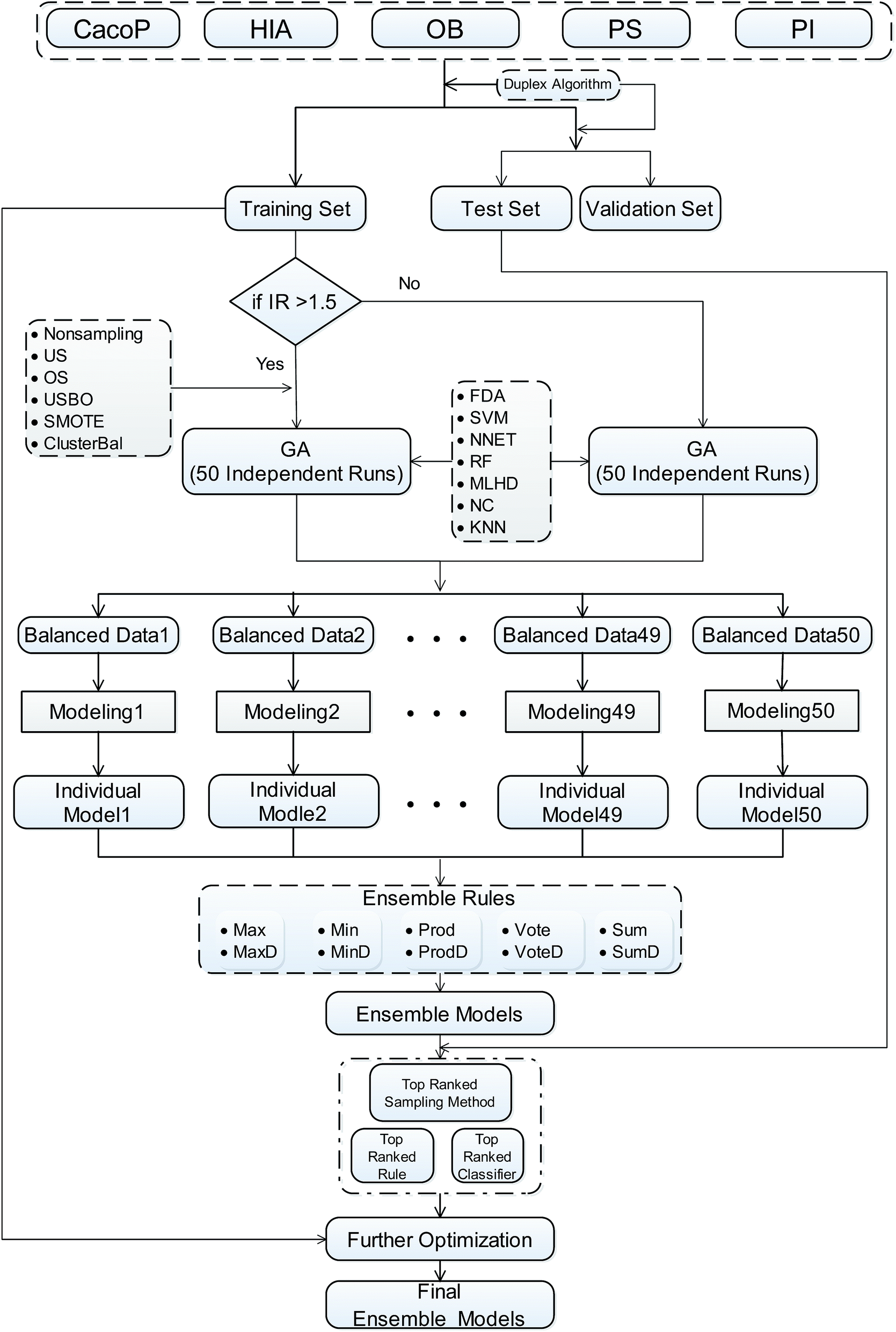 | ||
| Fig. 1 Workflow of the AECF. IR, imbalance ratio. US, undersampling. OS, oversampling. USBO, undersampling combined with bootstrapping. ClusterBal, cluster based balancing. RF, random forest. MLHD, maximum likelihood classifier. NC, nearest centroid classifier. | ||
• Undersampling (US): the majority class compounds are randomly eliminated to match the size of the minority class.
• Oversampling (OS): the minority class compounds are randomly sampled with replacement to match the size of the majority class.
• Synthetic minority oversampling technique (SMOTE): the synthetic samples for the minority class are created based on the k nearest neighbors of the same class, and the number of generated samples depends on the difference in size of the two classes. In this work, five nearest neighbors of the minority class were used to generate the synthetic samples.
• Undersampling combined with bootstrapping (USBO): this is a hybrid sampling method. The majority class compounds are undersampled and the minority class compounds are sampled by bootstrapping.
• Cluster based balancing (ClusterBal): this technique was presented by Sun et al.30 The idea of ClusterBal is that a balanced data set can be obtained by the combination of the subgroup of the majority class and the minority class. In this work, a k-means algorithm was employed to cluster the majority class into K groups. K depended on the IR, and K equaled the rounded IR to integer and no smaller than 2. Then one of these groups was randomly selected to be combined with the minority class, and the new balanced data set was constructed.
Further, nonsampling (NS) as a baseline method, which means that no sampling methods are applied, was also brought into the pool. Thus, after the number of balancing was predefined, multiple balanced subsets from original TRS could be acquired. However, when the TRS was judged as a balanced dataset, the multiple replications of TRS were created.
(i) Initial population of chromosomes with random descriptors: random descriptor sets were created from the original descriptor space. These selected descriptors made up a population of chromosomes, and were used as initially modelling feature vectors to develop base classifiers. Choosing too few descriptors can damage the performance of base classifiers, while using too many descriptors can lead to high computational cost as well as the potential for overfitting. In this study, the number of the selected descriptors was fixed at one twenty-fifth of the number of training instances and no larger than 20 during the GA evolution, and the population size was set to 20.
(ii) Chromosomes evaluation using fitness function: an internal 5-fold cross-validation (CV) was implemented to evaluate chromosomes' fitness during GA runs, and the AUC score (the area under the ROC curve) was taken as the fitness score of the chromosomes. The training set was randomly split into 5 non-overlapping subsets with equal size according to their categories. In each fold, one subset was held out for validation, and the rest were used to train the base classifier. Then this predictive model was applied to the validation subset. This procedure was repeated until every subset was used for validation. The pool of base classifiers includes seven popularly used machine learning techniques. The detailed information of these techniques is listed in Table 1, and the default parameters provided by the tool was used to construct classifiers.
(iii) Design of the GA operator: chromosomes with higher fitness in each generation were selected and then updated by the genetic operators: crossover and mutation. These procedures were repeated until the maximum generation was reached. In this study, the maximum generation was set to 100, and the other GA parameters were default according to Galgo package.51
At the conclusion of GA search, the informative descriptor subset with the highest fitness in the last generation was saved for each balanced training subset, and the corresponding individual model was built on the discriminative descriptor subset using a specific classifier. As a result, multiple individual models were achieved. There are two main advantages of using multiple GA runs in our scheme. First, the feature space can be reduced to improve the accuracy of base classifiers, resulting in individual models with high performance. Second, due to the stochastic of both the GA and data balancing methods, running the algorithm from a different training subset from original data set each time can yield a different discriminative descriptor subset, which promotes the diversity among individual models. Therefore, AECF is able to yield multiple individual models as accurate and diverse as those obtained with wrapper-based feature selection and data balancing.
| Rule | Strategy | Description |
|---|---|---|
| Max | S1 = argmax1≤i≤NP1i, S2 = argmax1≤i≤NP2i | Use the maximum predicted probability of N individual models for each class label |
| Min | S1 = argmin1≤i≤NP1i, S2 = argmin1≤i≤NP2i | Use the minimum predicted probability of N individual models for each class label |
| Prod | 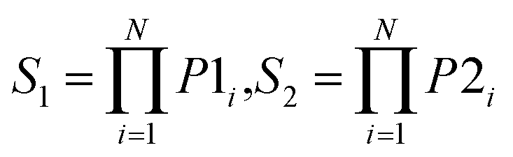 |
Use the product of predicted probability of N individual models for each class label |
| Vote |  |
For the ith model, if P1i ≥ P2i, class G1 gets a vote, otherwise, class G2 gets a vote |
| Sum | 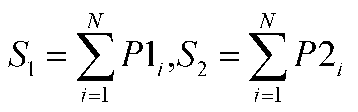 |
Use the summation of predicted probability of N individual models for each class label |
| MaxD |  |
Use the inverse of average distance to adjust the corresponding rule |
| MinD |  |
|
| ProdD | 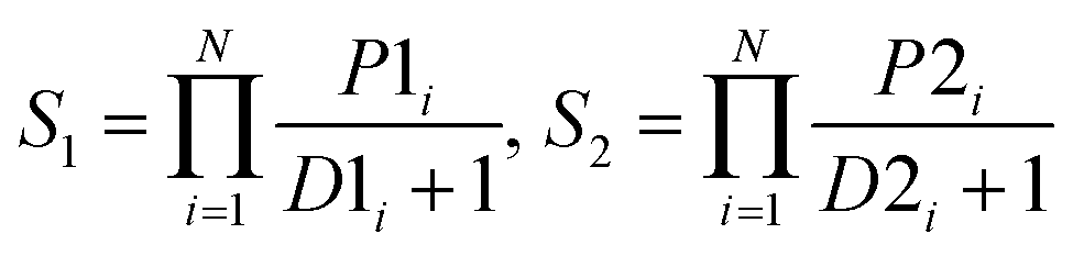 |
|
| VoteD | 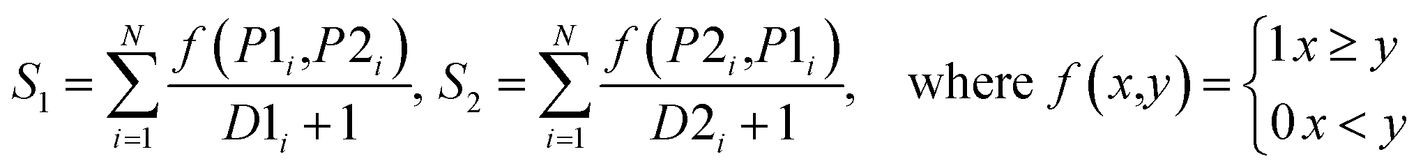 |
|
| SumD | 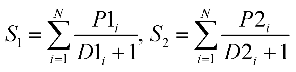 |
Considering that combination schemes tend to be data-specific (none produced the best results for all data sets). Therefore, in the first stage, all combinations of the methods from supplied pools including data balancing methods, base classifiers, and ensemble rules were tested. This resulted in 420 combinations for unbalanced data sets and 70 combinations for balanced data sets. For each combination, an ensemble model was established by the aggregation of multiple individual models. Then, the AUC score on TES was taken as the performance score. The combination with the highest performance was chosen as the adaptive selection. In the current investigation, the number of individual models was set to 50.
After obtaining the best combination of method pools, a further optimization can be invoked to find the best combination of individual models in the second stage, which yields the best ensemble performance. This selection of individual models focuses on finding the most efficient subset of ensembles, rather than combining all available individuals. In the second stage, a forward search algorithm (FSA) was designed. Initially, the goodness of each individual in the pool was evaluated. Individual models were ranked according to their fitness, from the best to the worse, and the top two individuals were firstly selected in the final ensemble. Then the individual model from the (sorted) input list was iteratively added into the ensemble where, at each step the ensemble was evaluated on the hold-out dataset. This procedure was repeated until no further improvements could be obtained. Here, a fitness function Q was defined for assessing the goodness of individual models as follows.
| Q = f(Perf, Div) | (1) |
 | (2) |
 | (3) |
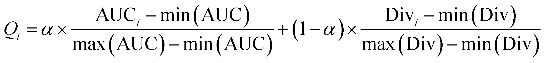 | (4) |
 | ||
| Fig. 2 Auto optimization for α by a rigorous 5-fold cross validation. Perf, the performance score of individual models. Div, the diversity score of individual models. Q, the fitness of individual models. | ||
Model evaluation
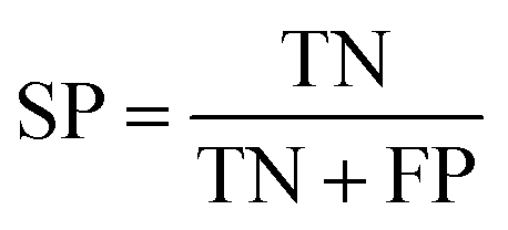
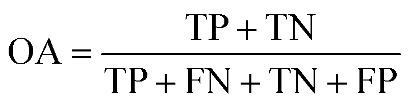
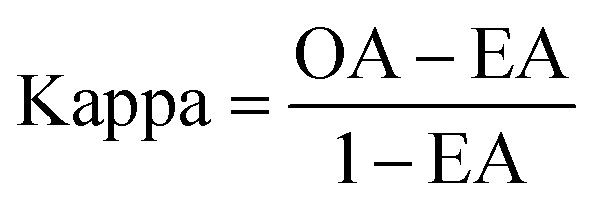
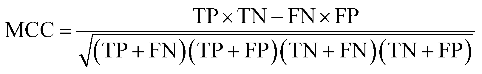
The performance of ensemble models was evaluated via the prediction of the two independent data set (test set and validation set). Considering the imbalanced classification task, several statistical metrics including specificity (SP), sensitivity (SE), overall accuracy (OA), kappa statistic, Matthews's correlation coefficient (MCC), and AUC were used as evaluation criteria. These metrics were calculated as follows:
 | (5) |
 | (6) |
 | (7) |
 | (8) |
 | (9) |
 | (10) |
Applicability domain (AD) analysis
It is necessary to define AD for delineation of interpolation space in which the model can make reliable predictions when applying a predictive model on a new dataset.61 Several different methodologies can be used for defining AD, including the projection approach62 and machine learning based approach.47,52 Our previous study11 showed that machine learning based approach was more appropriate for AD analysis than projection approach. In the presented work, we applied machine learning based approach to define AD. In this approach, the union of modeling descriptor sets of selected individual models were selected, and 100 shuffled training sets were created by randomly permuting these descriptors. Then 100 combined datasets were created, and each of them was constructed by merging the original training set and one shuffled set. An ensemble classification model was established to predict the probability of new compounds being members of the training set. Readers can refer to our previous work11 for implementation details.Tools
All calculations were performed with R-3.3.2 software. The packages used for implementing various base classifiers are presented in Table 1. SMOTE algorithm was implemented using DMwR package.63 Galgo51 package was used to perform GA. Caret package64 and boostr package65 was used to implement Bagging and Boosting algorithm, respectively.Results and discussions
Characterization of the data set
For each data set, only a small subset of calculated descriptors was remained for modeling after feature preprocessing, and data splitting resulted in fifty percent as TRS, twenty five percent as TES, and twenty five percent as VAS. The data characteristics are summarized in Table 3, where the number of compounds is listed in the parentheses following to the name of category. The calculated IRs for the different data sets are also shown. The results show that most of IRs are greater than the predefined threshold (IR = 1.5). Therefore, AECF handles these datasets (Cacop, HIA, OB, and PS) as unbalanced data except PI data.| Dataset | Subset | Descriptors | Class | IR | |
|---|---|---|---|---|---|
| Majority | Minority | ||||
| CacoP | TRS | 902 | CacoP+(461) | CacoP−(233) | 1.98 |
| TES | CacoP+(231) | CacoP−(116) | 1.99 | ||
| VAS | CacoP+(230) | CacoP−(116) | 1.98 | ||
| HIA | TRS | 677 | HIA+(316) | HIA−(51) | 6.20 |
| TES | HIA+(158) | HIA−(26) | 6.08 | ||
| VAS | HIA+(158) | HIA−(25) | 6.32 | ||
| OB | TRS | 940 | OB+(405) | OB−(134) | 3.02 |
| TES | OB+(202) | OB−(67) | 3.01 | ||
| VAS | OB+(202) | OB−(66) | 3.06 | ||
| PS | TRS | 880 | Substrate(276) | Nonsubstrate(172) | 1.60 |
| TES | Substrate(138) | Nonsubstrate(86) | 1.60 | ||
| VAS | Substrate(137) | Nonsubstrate(85) | 1.61 | ||
| PI | TRS | 832 | Inhibitor(620) | Noninhibitor(420) | 1.48 |
| TES | Inhibitor(310) | Noninhibitor(210) | 1.48 | ||
| VAS | Inhibitor(310) | Noninhibitor(209) | 1.48 | ||
In order to inspect the coverage of the chemical space of compounds, principal component analysis (PCA) was employed on each data set to visualize the data structure (Fig. 3). The total variance explained by the first two principal components was 15.8%, 15.2%, 14.8%, 15.0%, and 15.1% for CacoP, HIA, OB, PS, and PI, respectively. The majority and minority class points were coloured in blue and red, respectively. In Fig. 3, there was a trend for separation of two groups, which urged us to develop classification models. Moreover, it can be seen from the score plots that the majority class had more dispersion of the chemical properties than the minority class in most cases. On the other hand, for each data set, the distribution of the compounds seems to be well-balanced among the three data subsets, which illuminates the representative ability of samples in all subsets during duplex algorithm for splitting.
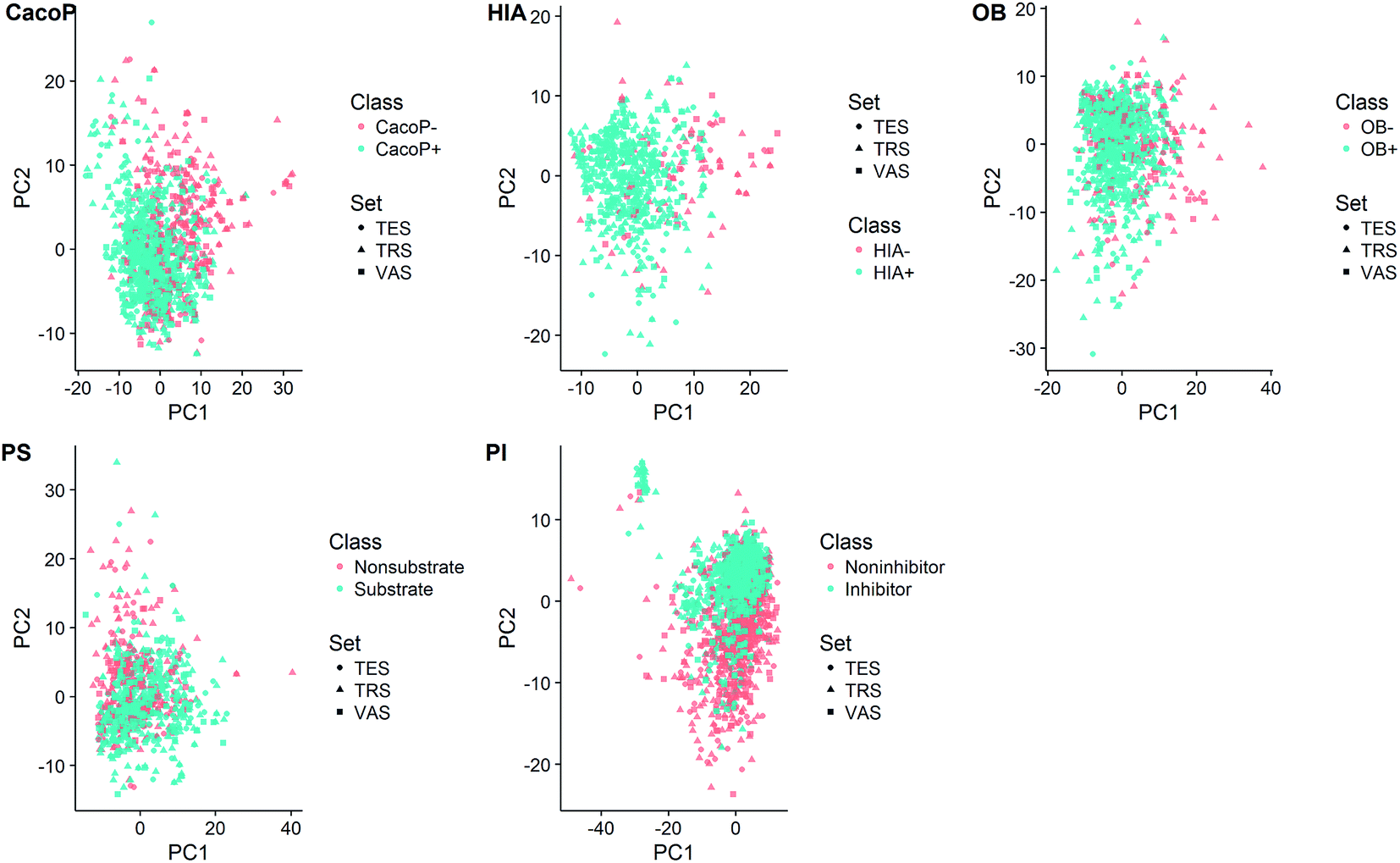 | ||
| Fig. 3 Score plot from PCA based on each data set. | ||
For each data set, profile analysis of individual molecular property was performed using Student's t-test or Fisher's exact test, and the corresponding P-values were calculated and ranked. As a result, there were 464, 282, 358, 324, and 488 statistically significant descriptors with a low P-value (P-value < 0.01) for CacoP, HIA, OB, PS, and PI data, respectively. The distributions of the top nine relevant descriptors between groups are shown in the ESI Fig. S1–S5.† We can see that DLDs whose name ending with a suffix “_DES” show high discriminability between groups for CacoP, HIA, and OB. While descriptors related to molecular hydrophobicity (Mlog![[thin space (1/6-em)]](https://www.rsc.org/images/entities/char_2009.gif) P) and the number of carbon atom in the molecule (PubchemFP12) are more discriminative for P-gp properties.
P) and the number of carbon atom in the molecule (PubchemFP12) are more discriminative for P-gp properties.
Development of AECF
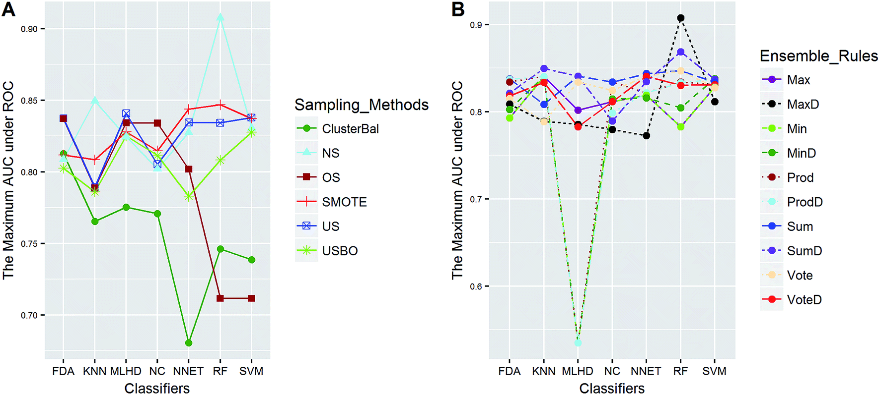
In this study, five data sets were divided into two types according to their IRs in AECF. CacoP, HIA, OB, and PS followed the route for tackling unbalanced datasets. The initial ensemble models were developed by the following procedures: data balancing, generating individual models, and combining individual models. Each method in each investigation pool was combined together to form the initial ensemble model, and the best combination in terms of AUC was picked out by AECF as the adaptive solution. In our framework, the default number of independent GA runs is 50, which means that each initial ensemble model was aggregated by 50 individual models during each combination. For unbalanced datasets, a total of 420 combinations were investigated. The maximum AUC scores of pairwise combinations for each data set are presented in Fig. 4–7. The results show that the different combination gained different performance. There were high degree of performance fluctuations among each pool of candidate methods. In order to investigate the relationships, a multiple linear regression model was built in terms of a connection between performance and methods for each data set, and the main effects and their two-way interaction effects were tested by analysis of variances. The corresponding P-values were calculated, and a term score (TS) was defined as the minus logarithm-transformed P-value.| TS = −log10(P-value) | (11) |
 | ||
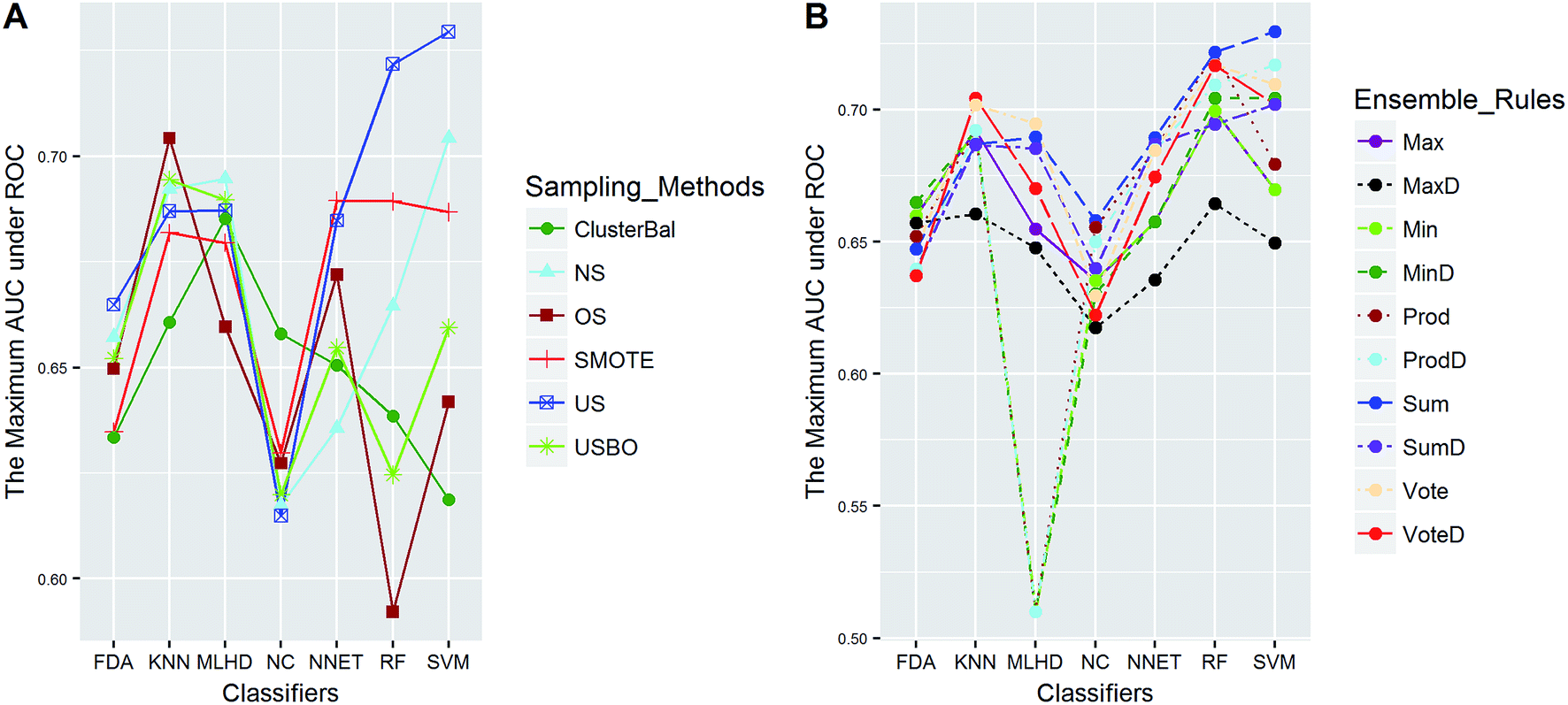
| Fig. 4 The maximum AUC scores of pairwise combinations for CacoP. (A) The combination of classifier and sampling method, and (B) the combination of classifier and ensemble rule. US, undersampling. OS, oversampling. USBO, undersampling combined with bootstrapping. ClusterBal, cluster based balancing. | ||
 | ||
| Fig. 5 The maximum AUC scores of pairwise combinations for HIA. (A) The combination of classifier and sampling method, and (B) the combination of classifier and ensemble rule. US, undersampling. OS, oversampling. USBO, undersampling combined with bootstrapping. ClusterBal, cluster based balancing. | ||
 | ||
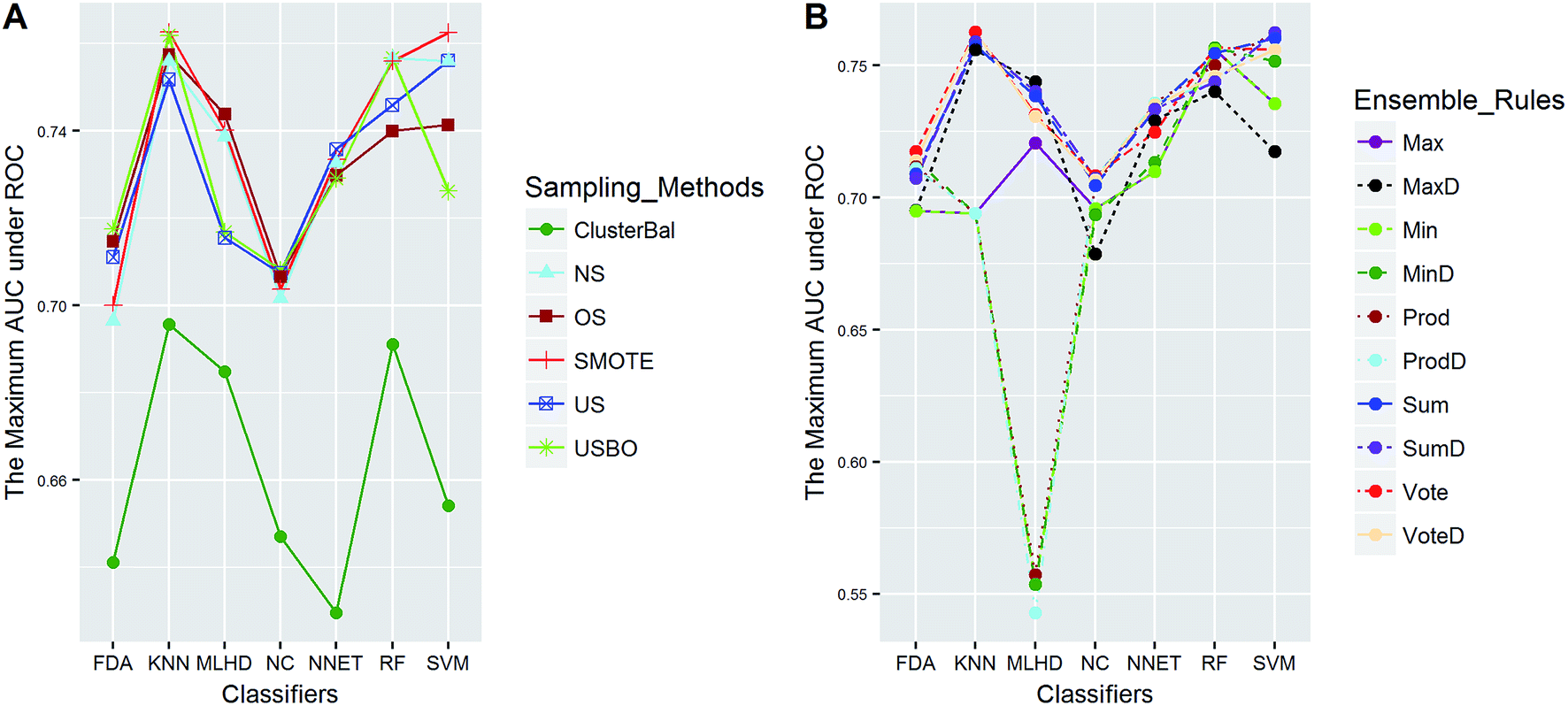
| Fig. 6 The maximum AUC scores of pairwise combinations for OB. (A) The combination of classifier and sampling method, and (B) the combination of classifier and ensemble rule. US, undersampling. OS, oversampling. USBO, undersampling combined with bootstrapping. ClusterBal, cluster based balancing. | ||
 | ||
| Fig. 7 The maximum AUC scores of pairwise combinations for PS. (A) The combination of classifier and sampling method, and (B) the combination of classifier and ensemble rule. US, undersampling. OS, oversampling. USBO, undersampling combined with bootstrapping. ClusterBal, cluster based balancing. | ||
Clearly, the more significant a term is, the higher TS it will get. Particularly, a term with P-value < 0.01 will have a TS > 2. The summarization of TS for each data set was shown in Fig. 8. All terms are statistically significant with TS greater than 2, which suggests that the choices of sampling methods, classifiers, and ensemble rules are key considerations to achieve better performance for these datasets. In most cases, SVM and RF presented better scores, while MLHD and NC were worse. Sampling method also played an important role in the development of predictive models. It is interesting that the baseline method (NS) was not always worst, on the contrary, the best performance was observed when it was combined with RF for HIA. The reasonable explanation may be due to the complicated interactions among the pools of candidate methods when AECF handles the unbalanced datasets.
 | ||
| Fig. 8 The summarization of TS for unbalanced datasets. | ||
The balanced dataset PI was tackled in the same way except that data balancing was skipped. The AUC scores of 70 combinations were recorded, and Fig. 9 presents the maximum scores of combinations between classifiers and ensemble rules. The main effects were also tested by the same way. The results show that the term of classifiers had a significant effect for performance with TS = 4.4, while the ensemble rules (TS = 1.0) didn't. Thus the choice of classifiers is more important than that of ensemble rules for PI data. The best score was obtained by the combination of SVM and VoteD.
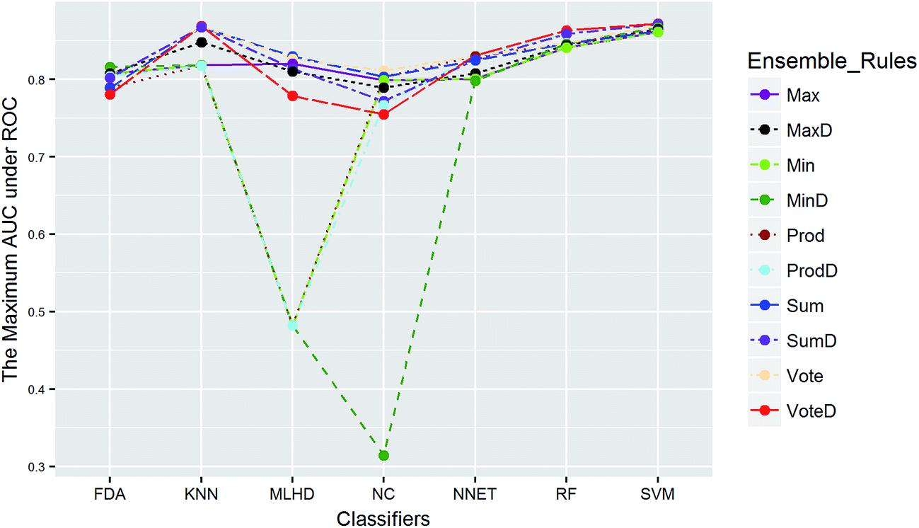 | ||
| Fig. 9 The maximum AUC scores of combinations between classifiers and ensemble rules for PI. | ||
Table 4 lists the adaptive solutions selected by AECF. To summarize, the adaptive routes of AECF for the construction of ensemble models are as follows:
| Data set | Sampling method | Classifier | Ensemble rule |
|---|---|---|---|
| CacoP | Undersampling | SVM | SumD |
| HIA | Nosampling | RF | MaxD |
| OB | Undersampling | SVM | Sum |
| PS | SMOTE | KNN | Vote |
| PI | Nosampling | SVM | VoteD |
• For CacoP data, US was used to balance the data, and individual models were generated by multiple GA-SVM runs. The ensemble model was built by aggregating individual outputs using SumD.
• For HIA data, individual models were generated by multiple GA-RF runs. The ensemble model was built by aggregating individual outputs using MaxD.
• For OB data, US was used to balance the data, and individual models were generated by multiple GA-SVM runs. The ensemble model was built by aggregating individual outputs using Sum.
• For PS data, SMOTE was used to balance the data, and individual models were generated by multiple GA-KNN runs. The ensemble model was built by aggregating individual outputs using Vote.
• For PI data, individual models were generated by multiple GA-SVM runs. The ensemble model was built by aggregating individual outputs using VoteD.
Then a five-times-repeated rigorous 5-fold cross validation combined with FSA described above was used in the second stage of optimization to find the optimal α automatically for each dataset. In the current stage, only TRS was used, and the range of α was set to [0,1]. The step was set to 0.1. With each value of α, using the adaptive routes determined previously, the ensemble models were built by aggregating 100 individual models in each fold validation. Fig. 10 shows the results of optimization procedure. It is apparent that the performance was more sensitive to the value of α. In most cases, a S-shaped-like curve was observed to describe the relationship between α and performance. In the range of α, neither the maximum nor the minimum could achieve the best performance for every data set. This indicates that the tradeoff between performance and diversity of individual models should be taken into consideration when constructing ensemble models. However, the relationships between α and ensemble size can be described as the reverse S-shaped-like curves in most cases. The larger α leads to smaller ensemble size. In other words, increasing the weight of performance in the fitness function Q helps to decrease the number of individuals to be aggregated. The α with the highest AUC was chosen automatically by AECF. Consequently, the optimal α was 0.6, 0.8, 0.8, 0.7, and 0.7 for CacoP, HIA, OB, PS, and PI, respectively. The optimal values were all greater than 0.5, which suggested that the performance was more important than the diversity during evaluating the fitness of individual models in our experiment.
 | ||
| Fig. 10 Optimization of α for (A) CacoP, (B) HIA, (C) OB, (D) PS, and (E) PI. | ||
After the optimization procedure, the ensemble model was rebuilt using the best combination of method pools based on TRS. 100 individual models were generated by multiple GA runs, and the ensemble size was automatically determined by FSA using the optimal α. Then the final (optimal) ensemble model was achieved. Due to the stochastic of generation of individual models, the procedure of constructing final ensemble model was repeated ten times. All the performance measures calculated on average over ten ensemble models for TES and VAS are shown in Table 5. We can see that, for all datasets, AECF shows the most discriminative power with AUC ranging from 0.7821–0.9182, MCC ranging from 0.5137–0.7887, OA ranging from 0.7792–0.9459, and kappa ranging from 0.5004–0.7856. To demonstrate the effectiveness of the optimization approach by AECF, the performances of the individual models and suboptimal ensemble models whose second stage of optimization were skipped are also reported. We can see that the final ensemble model (AECF) achieved the best performance in terms of all metrics in each data set. In contrast, the individual models were the worst. After applying our two-step adaptive optimization approach, the AUCs were raised by 6.36–26.99% and 2.09–8.04% compared to the individual models and suboptimal ensemble models, respectively. The distributions of ensemble size and AUC of ten AECF models for each data set are shown in Fig. 11. There were no clear relationships between ensemble size and performance. Although large ranges of ensemble size of final models were observed, the similar performances were obtained, which demonstrates the robustness of our approach.
| Data | Subset | Model | AUC | MCC | SE | SP | OA | Kappa |
|---|---|---|---|---|---|---|---|---|
| CacoP | TES | AECF | 0.8574 | 0.6935 | 0.8537 | 0.8612 | 0.8562 | 0.6889 |
| Suboptimal AECF | 0.8289 | 0.6370 | 0.8320 | 0.8259 | 0.8300 | 0.6327 | ||
| Individual model | 0.7643 | 0.5038 | 0.7396 | 0.7891 | 0.7561 | 0.4915 | ||
| VAS | AECF | 0.8602 | 0.6994 | 0.8574 | 0.8629 | 0.8592 | 0.6953 | |
| Suboptimal AECF | 0.8342 | 0.6439 | 0.8235 | 0.8448 | 0.8306 | 0.6375 | ||
| Individual model | 0.7703 | 0.5144 | 0.7362 | 0.8043 | 0.7590 | 0.5003 | ||
| HIA | TES | AECF | 0.9182 | 0.7887 | 0.9563 | 0.8800 | 0.9459 | 0.7856 |
| Suboptimal AECF | 0.8994 | 0.7236 | 0.9348 | 0.8640 | 0.9251 | 0.7160 | ||
| Individual model | 0.7953 | 0.686 | 0.9839 | 0.6067 | 0.9324 | 0.6715 | ||
| VAS | AECF | 0.8968 | 0.7404 | 0.9437 | 0.8500 | 0.9304 | 0.7357 | |
| Suboptimal AECF | 0.8782 | 0.6586 | 0.9063 | 0.8500 | 0.8984 | 0.6442 | ||
| Individual model | 0.7758 | 0.6737 | 0.9888 | 0.5628 | 0.9286 | 0.6501 | ||
| OB | TES | AECF | 0.7981 | 0.5295 | 0.7604 | 0.8358 | 0.7792 | 0.5027 |
| Suboptimal AECF | 0.7387 | 0.4302 | 0.7594 | 0.7179 | 0.7491 | 0.4157 | ||
| Individual model | 0.6285 | 0.2236 | 0.5965 | 0.6606 | 0.6125 | 0.1993 | ||
| VAS | AECF | 0.7821 | 0.5137 | 0.7990 | 0.7652 | 0.7907 | 0.5004 | |
| Suboptimal AECF | 0.7327 | 0.4369 | 0.8124 | 0.6530 | 0.7731 | 0.4325 | ||
| Individual model | 0.6413 | 0.2452 | 0.6092 | 0.6735 | 0.625 | 0.2194 | ||
| PS | TES | AECF | 0.8311 | 0.6738 | 0.8964 | 0.7659 | 0.8464 | 0.6709 |
| Suboptimal AECF | 0.7860 | 0.5677 | 0.8190 | 0.7529 | 0.7937 | 0.5672 | ||
| Individual model | 0.6772 | 0.3634 | 0.7914 | 0.5630 | 0.7039 | 0.3611 | ||
| VAS | AECF | 0.8139 | 0.6458 | 0.9022 | 0.7256 | 0.8344 | 0.6420 | |
| Suboptimal AECF | 0.7534 | 0.5026 | 0.7906 | 0.7163 | 0.7621 | 0.5020 | ||
| Individual model | 0.6848 | 0.3791 | 0.7974 | 0.5723 | 0.7109 | 0.3768 | ||
| PI | TES | AECF | 0.8898 | 0.7740 | 0.8900 | 0.8895 | 0.8898 | 0.7731 |
| Suboptimal AECF | 0.8669 | 0.7287 | 0.8732 | 0.8605 | 0.8681 | 0.7281 | ||
| Individual model | 0.8366 | 0.6708 | 0.8574 | 0.8157 | 0.8406 | 0.6703 | ||
| VAS | AECF | 0.8874 | 0.7699 | 0.8906 | 0.8842 | 0.8881 | 0.7691 | |
| Suboptimal AECF | 0.8688 | 0.7359 | 0.8887 | 0.8488 | 0.8726 | 0.7359 | ||
| Individual model | 0.8330 | 0.6673 | 0.8697 | 0.7962 | 0.8401 | 0.6671 |
 | ||
| Fig. 11 The distributions of (A) ensemble size and (B) AUC of ten AECF models for each data set. | ||
In order to investigate how the individuals in the ensemble complement each other to increase performance, the degree of complementarity of AECF was evaluated. The following calculations were all based on ten final ensemble models (EM).
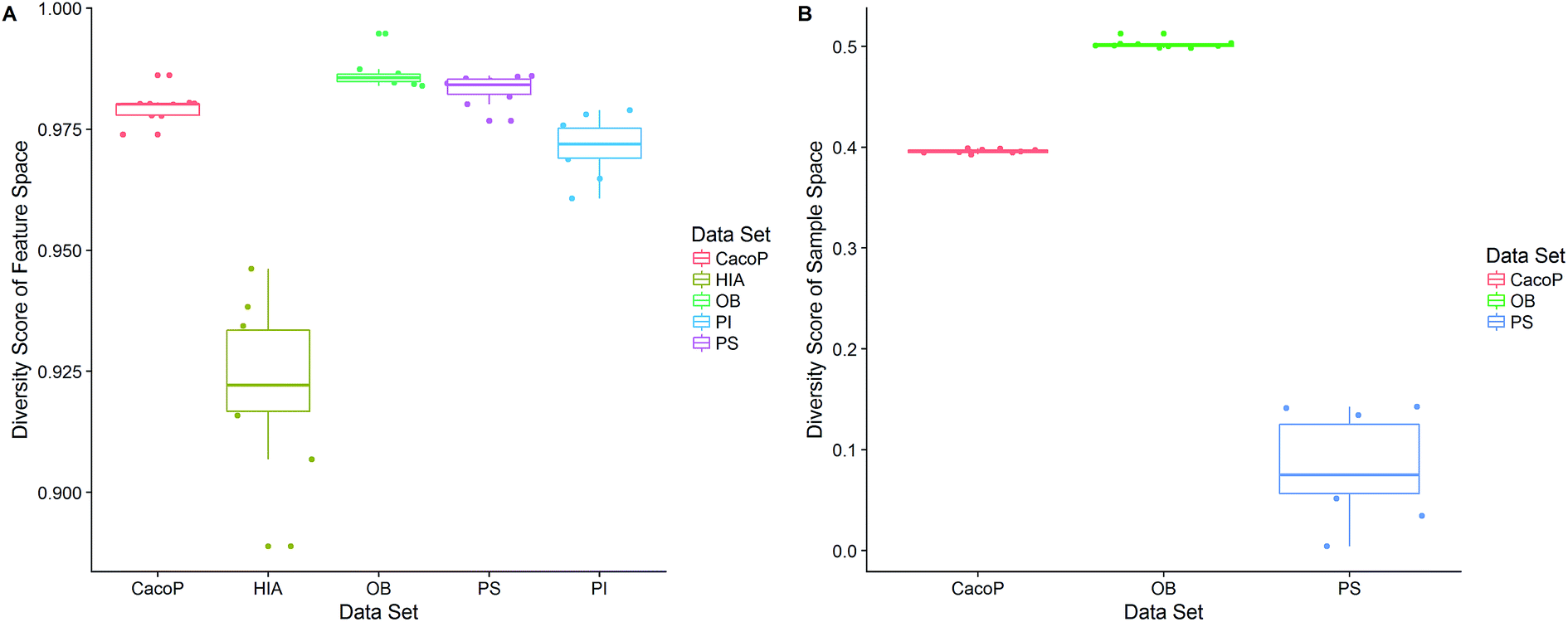
First, the degree of TRS that was utilized by AECF was analyzed. Both the sample and feature space coverage of individual models within final ensemble model were calculated for each data set. Fig. 12 presents the percentage of feature space coverage (PFSC) of each EM for each data set. We can see that there is a good linear relationship between ensemble size and the percentage of feature space coverage. Larger ensemble sizes led to larger PFSCs. The PFSCs were 0.08–0.29, 0.04–0.64, 0.10–0.47, 0.12–0.59, and 0.11–0.54 for CacoP, HIA, OB, PS, and PI, respectively. AECF achieved better performance by using only a small part (about 4–12%) of descriptors, which indicated that our approach successfully made a good optimization by eliminating the redundant features. Fig. 13 presents the percentage of sample space coverage (PSSC) of each EM for each data set (except HIA and PI where non-sampling was applied). The PSSCs were all 1.00 for PS. This means that the modeling data of AECF covered all TRS samples for PS. The PSSCs were 0.95–1.00 and 0.91–1.00 for CacoP and OB, respectively. Moreover, seven and five out of ten EMs were with the PSSC value 1.00 for CacoP and OB, respectively. Even though the ensemble sizes were small, the PSSCs were large. For instance, the PSSC of EM with the smallest ensemble size (4) for CacoP was still large (95%). The similar case could be found for OB. With the benefits of multiple data balancing and effective optimization strategy, AECF can make a better use of TRS samples despite selecting small number of individual models for aggregation.
 | ||
| Fig. 12 The percentage of feature space coverage of each EM for each data set. | ||
 | ||
| Fig. 13 The percentage of sample space coverage of each EM for CacoP, OB and PS data set. | ||
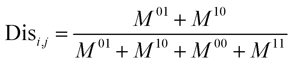
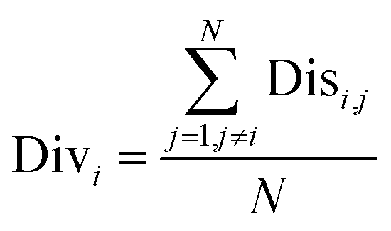
Next, the mechanism of diversity maintenance in individual models within AECF was further explored. A Jaccard distance (JD) was defined as follows to measure the diversity of both sample and feature space of individual models.
 | (12) |
 | ||
| Fig. 14 The distributions of diversity scores of (A) feature and (B) sample space. | ||
Last, a complementary index (CI)66 was defined as follows to quantify the degree of complementarity of individual models, and the relationships between the performance of EMs and the characteristics of their individual models were explored.
 | (13) |
CI is a pairwise metric, where Nij is the number of compounds with certain identification status by individual model i and j, and i,j ∈ {C,F} in which F denotes an individual model fails to classify the compound while C denotes it classify the compound correctly. In other words, CF is the number of compounds individual model i and j give inconsistent result, which is the situation of single fault. BF is the number of compounds both models fail. Then the degree of complementarity of EM can be calculated by averaging CI over all pairs. Fig. 15 presents the distribution of averaged CIs for each data set. It is observed that the averaged CIs of HIA and PI where nonsampling was applied were lower than those of others, which suggested that the additional diversity of sample space could help to promote the degree of complementarity. Moreover, a multiple linear regression model was established in terms of a connection between AUC scores and the characteristics (averaged CIs, the diversity score of sample and feature space) of EMs for the combined data set. Analysis of variance table (ESI Table S3†) of the regression model shows that all terms were statistically significant at the 0.05 level. This demonstrates that the performance of EM is associated with the complementarity and diversity of individuals. A rank based correlation analysis (Fig. 16) for each data set shows that all the correlation coefficients (CC) were positive, which indicate the positive relationships. Our findings are essentially consistent with the fact that the generation and maintenance of diversity in individuals help to improve the performance of EM, and AECF can effectively select complementary members to construct predictive models by our two-stage auto-adaptive optimization approach.
 | ||
| Fig. 15 The distributions of averaged CI for each data set. | ||
 | ||
| Fig. 16 CCs between AUC and the characteristics of EMs for each data set. | ||
Descriptor importance and contribution
In this work, the importance of descriptor was evaluated by the frequency that the number of times the descriptor was selected in individual models by multiple GA runs. The P-values were calculated as follows based on ten ensemble models using the binomial probabilities of descriptors being selected x times by GA runs.67
 | (14) |
P, LipoaffinityIndex, and MlogP) were more informative for identifying Pgp inhibitors, while some molecular fingerprints (PubchemFP12, MACCSFP129, PubchemFP500, KRFP18, MACCSFP49, and KRFP605) were more important for identifying Pgp substrates. It is particularly surprising that the ranks of contribution of some descriptors (e.g. MACCSFP70 and MACCSFP49) were quite different between the model based method and the univariate analysis. They were ranked lower, and even showed no significant by the univariate analysis. But they were important to construct predictive EMs, which suggests that there exists complex relationships between the descriptors and ADME characteristics. Due to the black-box property of EMs, the knowledge behind it remains unclear, and needs to be further explored in the future.
| Data Set | Descriptor | Times selected | P-value | RUSa |
|---|---|---|---|---|
| a RUS-ranks based on the univariate statistical test. | ||||
| CacoP | PSA_DES | 272 | <1.00 × 10−100 | 2 |
| QED_DES | 226 | <1.00 × 10−100 | 1 | |
| HBA_DES | 171 | 1.86 × 10−91 | 3 | |
| ETA_dEpsilon_D | 137 | 1.13 × 10−60 | 15 | |
| ALOGP_DES | 134 | 3.77 × 10−58 | 30 | |
| HBD_DES | 133 | 2.57 × 10−57 | 4 | |
| CrippenlogP |
119 | 4.84 × 10−46 | 10 | |
| AATSC1c | 115 | 5.77 × 10−43 | 9 | |
| MDEN.22 | 89 | 1.01 × 10⁻²⁴ | 101 | |
| XlogP |
85 | 3.26 × 10⁻²² | 24 | |
| HIA | MACCSFP49 | 652 | <1.00 × 10−100 | 30 |
| MDEO.11 | 480 | <1.00 × 10−100 | 25 | |
| PSA_DES | 459 | <1.00 × 10−100 | 3 | |
| QED_DES | 299 | <1.00 × 10−100 | 1 | |
| VC.4 | 452 | <1.00 × 10−100 | 228 | |
| HBA_DES | 190 | <1.00 × 10−100 | 2 | |
| VC.3 | 148 | 2.24 × 10−70 | 83 | |
| MATS4m | 123 | 2.41 × 10−49 | 181 | |
| MACCSFP70 | 108 | 6.69 × 10−38 | 672 | |
| nAcid | 105 | 9.93 × 10−36 | 122 | |
| OB | QED_DES | 114 | 6.97 × 10−44 | 1 |
| KRFP3757 | 90 | 1.33 × 10⁻²⁶ | 104 | |
| SubFP85 | 88 | 2.74 × 10⁻²⁵ | 22 | |
| KRFP346 | 87 | 1.22 × 10⁻²⁴ | 123 | |
| KRFP438 | 85 | 2.33 × 10⁻²³ | 309 | |
| MACCSFP30 | 85 | 2.33 × 10⁻²³ | 85 | |
| Lipinski failures | 83 | 4.22 × 10⁻²² | 3 | |
| VE3_D | 79 | 1.18 × 10⁻¹⁹ | 222 | |
| KRFP4557 | 75 | 2.68 × 10⁻¹⁷ | 330 | |
| PSA_DES | 70 | 1.71 × 10⁻¹⁴ | 6 | |
| PS | PubchemFP12 | 116 | 1.04 × 10−42 | 2 |
| MACCSFP129 | 98 | 7.49 × 10⁻³⁰ | 1 | |
| PubchemFP500 | 76 | 2.58 × 10⁻¹⁶ | 269 | |
| KRFP18 | 69 | 1.36 × 10⁻¹² | 34 | |
| maxHCsats | 68 | 4.37 × 10⁻¹² | 35 | |
| MACCSFP49 | 66 | 4.28 × 10⁻¹¹ | 467 | |
| JGI10 | 63 | 1.17 × 10⁻⁹ | 60 | |
| SpMAD_Dzs | 62 | 3.40 × 10⁻⁹ | 28 | |
| Lipoaffinity index | 61 | 9.74 × 10⁻⁹ | 76 | |
| KRFP605 | 60 | 2.74 × 10⁻⁸ | 36 | |
| PI | CrippenlogP |
245 | <1.00 × 10−100 | 6 |
| Lipoaffinity index | 257 | <1.00 × 10−100 | 3 | |
| MlogP |
305 | <1.00 × 10−100 | 1 | |
| SpMin3_Bhs | 200 | <1.00 × 10−100 | 5 | |
| WPATH | 197 | <1.00 × 10−100 | 82 | |
| SubFP84 | 169 | 2.46 × 10−84 | 83 | |
| SpMAD_Dt | 145 | 3.21 × 10−63 | 31 | |
| MDEC.23 | 141 | 6.89 × 10−60 | 2 | |
| PubchemFP192 | 134 | 3.38 × 10−54 | 15 | |
| ATSC0p | 128 | 1.83 × 10−49 | 13 | |
Comparison with other algorithms and models
In the following section, our results of prediction performance were compared tentatively with those of published literatures. It was not easy to make a direct comparison between ours and those of previously published classification models because of the particularity of the data used and unbalance degree. Table 7 summarizes the previously published classification models for each property. Since many literatures developed more than one models, the best performances were reported. It is apparent that the present work was based on the largest data set, and achieved the best performance in some cases. Although some models produced better performances, they were based on a relatively small amount of compounds, and their classification cutoff values might be unreasonable in practice, or they were validated by a very small independent data set. For PI data, compared to our previously study,11 AECF achieved better performances than the ensemble of different classifiers for the same independent data set.| Data set | Model | No. of compounds | Performancea | Reference |
|---|---|---|---|---|
| a The accuracy of independent test data. | ||||
| CacoP | LDA | 51 | 88.90% | 68 |
| KNN | 712 | 75.5–88.5% | 69 | |
| LDA | 157 | 84.20% | 1 | |
| LDA | 146 | 83.30% | 70 | |
| GLDA | 674 | 78–82% | 71 | |
| 3PRule | 1279 | 70.6–72.9% | 2 | |
| AECF | 1387 | 85.77% | Ours | |
| HIA | SVM | 578 | 98.00% | 19 |
| ANN | 367 | 75.00% | 72 | |
| PLSDA, CART | 225 | 84.00% | 13 | |
| SVM | 578 | 99.00% | 73 | |
| CART, ANN | 458 | 79.00–91.00% | 3 | |
| CART | 645 | 74.2–85.3% | 4 | |
| AECF | 734 | 93.82% | Ours | |
| OB | ROC | 184 | 74.00% | 74 |
| 21 models | 969 | 71.00% | 22 | |
| RF,SVM,KNN | 995 | 76.00% | 5 | |
| AECF | 1076 | 78.49% | Ours | |
| PS | SVM | 332 | 69.24% | 75 |
| SVM,RF,KNN | 484 | 70.00% | 16 | |
| SVM,KNN,CART | 195 | 81.00% | 76 | |
| SVM | 99 | 80.00% | 77 | |
| SVM | 332 | 88.00% | 12 | |
| NB | 822 | 83.50% | 78 | |
| AECF | 894 | 84.04% | Ours | |
| PI | PLSDA | 325 | 72.40% | 79 |
| NB | 609 | 82.20% | 80 | |
| RP,NB | 1273 | 81.20% | 14 | |
| PLSDA,LDA | 1275 | 85.0–86.0% | 81 | |
| KNN,SVM,RF | 1935 | 75.00% | 16 | |
| SOM,NNET | 206 | 80.80% | 15 | |
| SVM | 1275 | 86.80% | 82 | |
| SVM,KNN,RF | 1954 | 73.0–82.0% | 17 | |
| Ensemble(FDA,RF,SVM) Models | 2079 | 85.50% | 11 | |
| AECF | 2079 | 88.89% | Ours | |
Moreover, our proposed approach was compared with two representative ensemble methods Bagging and Boosting. Bagging based ensemble models were built by training several classifiers with bootstrapped version of the original training data, while Boosting introduced a re-weighting technique to reduce the bias towards the majority class. In this work, the best individual model within the final AECF was picked out as the base classifier. The number of bootstrap samples and the number of iterations of boosting were optimized by a 10-fold CV, and the other parameters were set to default. Table 8 summarizes the average performances of ten models for each data set. It is clear that AECF achieved the best performances in terms of AUC, MCC, and Kappa for all data sets. Bagging and Boosting produced similar performances, and they were superior to the individual models in most cases. Then a pairwise Kruskal–Wallis rank sum test was used to clarify the difference of performances of these methods regarding to AUC. The P-values adjusted by false discovery rate are presented in ESI Table S4,† which supports AECF gains the best performance. The results indicate that there were significant differences between representative ensemble methods and AECF with low P-values (P-value < 0.001), which implied AECF significantly outperformed the others for these data sets.
| Data set | Subset | Model | AUC | MCC | SE | SP | OA | Kappa |
|---|---|---|---|---|---|---|---|---|
| CacoP | TES | SVM-Bagging | 0.7785 | 0.5445 | 0.8156 | 0.7414 | 0.7908 | 0.5422 |
| SVM-Boosting | 0.7866 | 0.5823 | 0.8766 | 0.6966 | 0.8164 | 0.5816 | ||
| AECF | 0.8574 | 0.6935 | 0.8537 | 0.8612 | 0.8562 | 0.6889 | ||
| VAS | SVM-Bagging | 0.7899 | 0.5650 | 0.8143 | 0.7655 | 0.7980 | 0.5616 | |
| SVM-Boosting | 0.7891 | 0.5847 | 0.8713 | 0.7069 | 0.8162 | 0.5840 | ||
| AECF | 0.8602 | 0.6994 | 0.8574 | 0.8629 | 0.8592 | 0.6953 | ||
| HIA | TES | RF-Bagging | 0.8643 | 0.6432 | 0.9127 | 0.8160 | 0.8995 | 0.6316 |
| RF-Boosting | 0.8251 | 0.7255 | 0.9823 | 0.6680 | 0.9393 | 0.7154 | ||
| AECF | 0.8968 | 0.7404 | 0.9437 | 0.8500 | 0.9304 | 0.7357 | ||
| VAS | RF-Bagging | 0.8430 | 0.5902 | 0.8899 | 0.7962 | 0.8766 | 0.5746 | |
| RF-Boosting | 0.8097 | 0.7012 | 0.9810 | 0.6385 | 0.9326 | 0.6905 | ||
| AECF | 0.9182 | 0.7887 | 0.9563 | 0.8800 | 0.9459 | 0.7856 | ||
| OB | TES | SVM-Bagging | 0.6456 | 0.2776 | 0.7807 | 0.5104 | 0.7134 | 0.2757 |
| SVM-Boosting | 0.6075 | 0.2546 | 0.8955 | 0.3194 | 0.7520 | 0.2442 | ||
| AECF | 0.7981 | 0.5295 | 0.7604 | 0.8358 | 0.7792 | 0.5027 | ||
| VAS | SVM-Bagging | 0.6591 | 0.3069 | 0.8015 | 0.5167 | 0.7313 | 0.3053 | |
| SVM-Boosting | 0.6348 | 0.3144 | 0.9030 | 0.3667 | 0.7709 | 0.3040 | ||
| AECF | 0.7821 | 0.5137 | 0.7990 | 0.7652 | 0.7907 | 0.5004 | ||
| PS | TES | KNN-Bagging | 0.7128 | 0.4186 | 0.6930 | 0.7326 | 0.7174 | 0.4161 |
| KNN-Boosting | 0.6660 | 0.3378 | 0.5616 | 0.7703 | 0.6902 | 0.3366 | ||
| AECF | 0.8311 | 0.6738 | 0.8964 | 0.7659 | 0.8464 | 0.6709 | ||
| VAS | KNN-Bagging | 0.6951 | 0.3903 | 0.6259 | 0.7642 | 0.7113 | 0.3895 | |
| KNN-Boosting | 0.6726 | 0.3598 | 0.5400 | 0.8051 | 0.7036 | 0.3553 | ||
| AECF | 0.8139 | 0.6458 | 0.9022 | 0.7256 | 0.8344 | 0.6420 | ||
| PI | TES | SVM-Bagging | 0.8328 | 0.6574 | 0.8433 | 0.8223 | 0.8308 | 0.6544 |
| SVM-Boosting | 0.8329 | 0.6617 | 0.8190 | 0.8468 | 0.8356 | 0.6610 | ||
| AECF | 0.8898 | 0.7740 | 0.8900 | 0.8895 | 0.8898 | 0.7731 | ||
| VAS | SVM-Bagging | 0.8407 | 0.6746 | 0.8402 | 0.8413 | 0.8408 | 0.6732 | |
| SVM-Boosting | 0.8260 | 0.6528 | 0.7895 | 0.8626 | 0.8331 | 0.6527 | ||
| AECF | 0.8874 | 0.7699 | 0.8906 | 0.8842 | 0.8881 | 0.7691 |
Relationships between OB and other ADME properties
The relationships between OB and other ADME properties were analyzed by a Fisher's exact test based on the common compounds presented in the datasets. Table 9 presents the contingency table between OB and other ADME properties, and the corresponding standardized residuals are also reported. Although the number of common compounds between groups was small, the significant associations of OB–CacoP and OB–HIA were observed with low P values(<0.0001). Large positive standardized residual (3.44 greater than 1.96) of CacoP- and OB-indicated that when compounds belonged to CacoP–, they had significantly more likelihood to be OB–, and the similar occurrence was observed in OB–HIA. These finds suggested that the positive associations of OB–CacoP and OB–HIA were mainly driven by the undesirable class compounds. So the predictions of CacoP and HIA are meaningful toward the prediction of OB. However, the associations between OB and P-gp properties were not found to be statistically significant (P values more than 0.05 by Fisher's exact test).| ADME properties | Class | OB | P value# | |
|---|---|---|---|---|
| OB+ | OB- | |||
| a # P values were obtained using Fisher's exact test. | ||||
| CacoP | CacoP+ | 123 | 15 | 1.68 × 10⁻⁵ |
| Std residual | 1.101 | −2.252 | ||
| CacoP- | 36 | 23 | ||
| Std residual | −1.684 | 3.444 | ||
| HIA | HIA+ | 133 | 7 | 1.67 × 10⁻⁷ |
| Std residual | 0.615 | −1.852 | ||
| HIA- | 3 | 8 | ||
| Std residual | −2.194 | 6.608 | ||
| PS | Substrate | 33 | 6 | 0.557 |
| Std residual | 0.227 | −0.474 | ||
| Nonsubstrate | 28 | 8 | ||
| Std residual | −0.237 | 0.494 | ||
| PI | Inhibitor | 1 | 2 | 0.121 |
| Std residual | −0.873 | 1.633 | ||
| Noninhibitor | 41 | 10 | ||
| Std residual | 0.212 | −0.396 | ||
AD analysis
It is necessary to examine a model's predictive reliability for practical purpose. As mentioned above, an ensemble classification model was used to measure the reliability characterized by the chemical domain for each data set. This AD EM was developed based on the molecular descriptors selected by the final AECF, and the values of the predicted probability were output to distinguish Inside-AD and Outside-AD. The default cutoff value was set to 0.5, so that compounds with a predicted probability > 0.5 were labelled as Inside-AD and vice versa. As a result, all compounds from the two independent subsets (TES and VAS) were labelled as Inside-AD for each data set at the default cutoff value (COF), which illustrated that the similar chemical coverage to TRS was achieved by duplex algorithm.Furthermore, the effect of the COFs of the AD probability on the model performance was investigated. In this way, COF varied from 0.5 to 0.9, and the performance metrics were recalculated on the Inside-AD compounds. Table 10 presents the results for each data set. We can see that higher performances were achieved when COFs were also higher. It is apparent that increasing COF decreased the number of Inside-AD compounds that the model covered, but in general, increased the performance of classification models.
| Dataset | Subset | COF | NCa | The performance of Inside-AD compounds | ||||||
|---|---|---|---|---|---|---|---|---|---|---|
| Inside | Outside | MCC | AUC | SE | SP | OA | Kappa | |||
| a The number of compounds.b Not available. | ||||||||||
| CacoP | TES | 0.5 | 347 | 0 | 0.701 | 0.860 | 0.866 | 0.853 | 0.862 | 0.698 |
| 0.6 | 332 | 15 | 0.721 | 0.868 | 0.876 | 0.860 | 0.870 | 0.719 | ||
| 0.7 | 297 | 50 | 0.729 | 0.873 | 0.870 | 0.875 | 0.872 | 0.726 | ||
| 0.8 | 211 | 136 | 0.775 | 0.897 | 0.893 | 0.901 | 0.896 | 0.773 | ||
| 0.9 | 76 | 271 | 0.826 | 0.921 | 0.922 | 0.920 | 0.921 | 0.825 | ||
| VAS | 0.5 | 346 | 0 | 0.691 | 0.853 | 0.870 | 0.836 | 0.858 | 0.690 | |
| 0.6 | 333 | 13 | 0.713 | 0.865 | 0.874 | 0.856 | 0.868 | 0.711 | ||
| 0.7 | 285 | 61 | 0.740 | 0.878 | 0.876 | 0.880 | 0.877 | 0.737 | ||
| 0.8 | 198 | 148 | 0.760 | 0.894 | 0.863 | 0.925 | 0.884 | 0.752 | ||
| 0.9 | 72 | 274 | 0.854 | 0.937 | 0.915 | 0.960 | 0.931 | 0.851 | ||
| HIA | TES | 0.5 | 184 | 0 | 0.803 | 0.921 | 0.962 | 0.880 | 0.951 | 0.802 |
| 0.6 | 168 | 16 | 0.780 | 0.912 | 0.960 | 0.864 | 0.948 | 0.778 | ||
| 0.7 | 131 | 53 | 0.838 | 0.951 | 0.964 | 0.938 | 0.960 | 0.834 | ||
| 0.8 | 64 | 120 | 1.000 | 1.000 | 1.000 | 1.000 | 1.000 | 1.000 | ||
| 0.9 | 21 | 163 | 1.000 | 1.000 | 1.000 | 1.000 | 1.000 | 1.000 | ||
| VAS | 0.5 | 183 | 0 | 0.731 | 0.907 | 0.930 | 0.885 | 0.924 | 0.722 | |
| 0.6 | 172 | 11 | 0.742 | 0.906 | 0.938 | 0.875 | 0.929 | 0.736 | ||
| 0.7 | 126 | 57 | 0.702 | 0.885 | 0.929 | 0.842 | 0.916 | 0.695 | ||
| 0.8 | 66 | 117 | 0.821 | 0.932 | 0.941 | 0.923 | 0.938 | 0.817 | ||
| 0.9 | 12 | 171 | 1.000 | 1.000 | 1.000 | 1.000 | 1.000 | 1.000 | ||
| OB | TES | 0.5 | 269 | 0 | 0.534 | 0.797 | 0.787 | 0.806 | 0.792 | 0.516 |
| 0.6 | 234 | 35 | 0.547 | 0.799 | 0.799 | 0.800 | 0.799 | 0.532 | ||
| 0.7 | 162 | 107 | 0.578 | 0.801 | 0.857 | 0.744 | 0.827 | 0.576 | ||
| 0.8 | 88 | 181 | 0.529 | 0.795 | 0.773 | 0.818 | 0.784 | 0.506 | ||
| 0.9 | 19 | 250 | 0.889 | 0.962 | 0.923 | 1.000 | 0.947 | 0.883 | ||
| VAS | 0.5 | 268 | 0 | 0.514 | 0.788 | 0.772 | 0.803 | 0.780 | 0.492 | |
| 0.6 | 240 | 28 | 0.525 | 0.788 | 0.787 | 0.790 | 0.788 | 0.510 | ||
| 0.7 | 172 | 96 | 0.616 | 0.840 | 0.823 | 0.857 | 0.831 | 0.598 | ||
| 0.8 | 82 | 186 | 0.659 | 0.855 | 0.852 | 0.857 | 0.854 | 0.649 | ||
| 0.9 | 16 | 252 | 0.537 | 0.933 | 0.867 | 1.000 | 0.875 | 0.448 | ||
| PS | TES | 0.5 | 224 | 0 | 0.677 | 0.840 | 0.812 | 0.869 | 0.847 | 0.677 |
| 0.6 | 216 | 8 | 0.676 | 0.839 | 0.805 | 0.872 | 0.847 | 0.675 | ||
| 0.7 | 177 | 47 | 0.710 | 0.848 | 0.780 | 0.917 | 0.865 | 0.708 | ||
| 0.8 | 98 | 126 | 0.629 | 0.805 | 0.696 | 0.915 | 0.854 | 0.628 | ||
| 0.9 | 31 | 193 | NAb | NAb | NAb | 1.000 | 1.000 | NAb | ||
| VAS | 0.5 | 222 | 0 | 0.646 | 0.813 | 0.721 | 0.906 | 0.835 | 0.642 | |
| 0.6 | 215 | 7 | 0.641 | 0.809 | 0.707 | 0.910 | 0.833 | 0.636 | ||
| 0.7 | 155 | 67 | 0.609 | 0.790 | 0.672 | 0.909 | 0.819 | 0.602 | ||
| 0.8 | 82 | 140 | 0.693 | 0.813 | 0.656 | 0.970 | 0.867 | 0.675 | ||
| 0.9 | 15 | 207 | 0.713 | 0.786 | 0.571 | 1.000 | 0.903 | 0.674 | ||
| PI | TES | 0.5 | 520 | 0 | 0.774 | 0.889 | 0.881 | 0.897 | 0.890 | 0.774 |
| 0.6 | 514 | 6 | 0.779 | 0.891 | 0.879 | 0.902 | 0.893 | 0.778 | ||
| 0.7 | 460 | 60 | 0.774 | 0.888 | 0.867 | 0.909 | 0.893 | 0.774 | ||
| 0.8 | 290 | 230 | 0.778 | 0.891 | 0.842 | 0.939 | 0.914 | 0.778 | ||
| 0.9 | 121 | 399 | 0.805 | 0.915 | 0.857 | 0.972 | 0.959 | 0.804 | ||
| VAS | 0.5 | 519 | 0 | 0.757 | 0.880 | 0.866 | 0.894 | 0.882 | 0.757 | |
| 0.6 | 513 | 6 | 0.753 | 0.878 | 0.863 | 0.893 | 0.881 | 0.753 | ||
| 0.7 | 461 | 58 | 0.768 | 0.884 | 0.854 | 0.914 | 0.892 | 0.768 | ||
| 0.8 | 311 | 208 | 0.754 | 0.871 | 0.800 | 0.942 | 0.904 | 0.754 | ||
| 0.9 | 113 | 406 | 0.637 | 0.771 | 0.563 | 0.979 | 0.920 | 0.623 | ||
External validation
After demonstrating the ADME prediction ability of AECF, we applied our models to predict ADME properties of the compounds from DrugBank 5.0 (ref. 83) (http://www.drugbank.ca) database. DrugBank database provides many ADMET related properties of compounds. In this work, 1925 approved compounds were chosen as an external database for prediction application. After removing the duplicates and overlapping compounds, 1793 unique compounds were prepared, and those compounds whose prediction probabilities are greater than or equal to 0.7 were extracted for investigation. As a result, there were 652, 1398, 1307, 814, and 974 compounds for predicting their ADME property of CacoP, HIA, OB, PS, and PI, respectively. Then the probability that the query compound was a member of the modeling data set was predicted by the corresponding AD model. Table 11 shows the predictions of our models for Inside-AD compounds based on the different COFs of the AD probability. Although classification cutoff values of CacoP and OB in DrugBank database were different from ours, overall, our predictive models achieved better concordance with DrugBank predictions. As expected, better performances were achieved based on the higher COFs at the expense of AD coverage in most cases. It is particularly surprising that the best performance in terms of AUC was obtained when COF equaled 0.6 for PS. These results suggested that an appropriate balance between the predictive reliability and the size of AD should be taken into consideration when determining a COF for practical application.| Property | COF | NCa | The performance of Inside-AD compounds | ||||||
|---|---|---|---|---|---|---|---|---|---|
| Total | Inside-AD | MCC | AUC | SE | SP | OA | Kappa | ||
| a The number of compounds.b Classification cutoff values of these properties in DrugBank database are different from ours. | |||||||||
| CacoPb | 0.5 | 652 | 634 | 0.6956 | 0.8237 | 0.6621 | 0.9853 | 0.8360 | 0.6624 |
| 0.6 | 652 | 599 | 0.7154 | 0.8359 | 0.6873 | 0.9846 | 0.8481 | 0.6871 | |
| 0.7 | 652 | 450 | 0.7788 | 0.8716 | 0.7590 | 0.9843 | 0.8867 | 0.7631 | |
| 0.8 | 652 | 242 | 0.8680 | 0.9172 | 0.8409 | 0.9935 | 0.9380 | 0.8617 | |
| 0.9 | 652 | 40 | 1.0000 | 1.0000 | 1.0000 | 1.0000 | 1.0000 | 1.0000 | |
| HIA | 0.5 | 1398 | 1347 | 0.6118 | 0.9015 | 0.9225 | 0.8805 | 0.8849 | 0.5683 |
| 0.6 | 1398 | 1187 | 0.6314 | 0.9040 | 0.9083 | 0.8997 | 0.9006 | 0.5963 | |
| 0.7 | 1398 | 820 | 0.7293 | 0.9235 | 0.9070 | 0.9401 | 0.9366 | 0.7149 | |
| 0.8 | 1398 | 407 | 0.8176 | 0.9373 | 0.9048 | 0.9699 | 0.9631 | 0.8146 | |
| 0.9 | 1398 | 86 | 0.8622 | 0.9311 | 0.8750 | 0.9872 | 0.9767 | 0.8622 | |
| OBb | 0.5 | 1307 | 1210 | 0.3384 | 0.7252 | 0.9261 | 0.5243 | 0.5917 | 0.2355 |
| 0.6 | 1307 | 1036 | 0.3573 | 0.7369 | 0.9209 | 0.5530 | 0.6158 | 0.2590 | |
| 0.7 | 1307 | 667 | 0.4042 | 0.7596 | 0.9355 | 0.5838 | 0.6492 | 0.3094 | |
| 0.8 | 1307 | 291 | 0.5245 | 0.7925 | 0.9136 | 0.6714 | 0.7388 | 0.4737 | |
| 0.9 | 1307 | 33 | 0.5164 | 0.7727 | 0.8182 | 0.7273 | 0.7576 | 0.5000 | |
| PS | 0.5 | 814 | 776 | 0.7358 | 0.8868 | 0.9221 | 0.8515 | 0.8737 | 0.7254 |
| 0.6 | 814 | 737 | 0.7482 | 0.8959 | 0.9430 | 0.8487 | 0.8779 | 0.7348 | |
| 0.7 | 814 | 520 | 0.7355 | 0.8914 | 0.9430 | 0.8398 | 0.8712 | 0.7199 | |
| 0.8 | 814 | 241 | 0.6447 | 0.8694 | 0.9259 | 0.8128 | 0.8382 | 0.6135 | |
| 0.9 | 814 | 65 | 0.3898 | 0.7639 | 0.7778 | 0.7500 | 0.7538 | 0.3384 | |
| PI | 0.5 | 974 | 919 | 0.6322 | 0.7329 | 0.4699 | 0.9960 | 0.9010 | 0.5821 |
| 0.6 | 974 | 885 | 0.6476 | 0.7432 | 0.4906 | 0.9959 | 0.9051 | 0.6017 | |
| 0.7 | 974 | 708 | 0.7315 | 0.8011 | 0.6071 | 0.9950 | 0.9336 | 0.7072 | |
| 0.8 | 974 | 319 | 0.8429 | 0.8958 | 0.8033 | 0.9884 | 0.9530 | 0.8389 | |
| 0.9 | 974 | 55 | 1.0000 | 1.0000 | 1.0000 | 1.0000 | 1.0000 | 1.0000 | |
Limitations and future work
Although AECF makes encouraging predictive performance, it has some limitations and shares common weakness associated with EM classification task. First, although our prediction work was developed based on the large databases, the compounds were actually from various literature sources, increasing the risk of erroneous judgment. So such large and compatible classification data sets are still encouraged to yield more reliable predictions. Second, AECF shows reliable performances on ADME datasets with the IR range of 1.48–6.32. However, this cannot guarantee that the same performance can be achieved on a more unbalanced dataset when a reasonable classification cutoff value is determined. Therefore, the performance on a higher degree of unbalanced dataset needs to be investigated in the future. Third, AECF is a GA based ensemble approach, and multiple runs of GA is performed in order to keep diversity and quality of individual model. The number of GA runs depends on the number of balanced datasets to construct individual models. However, the exact number is hard to decide. More runs may result in a more reliable and extensive individual model pool at a cost of more computation time. On the other hand, our results demonstrate that the optimal solutions for modeling are data-specific, so all combinations of the methods from supplied method pools including data balancing methods, base classifiers, and ensemble rules need to be investigated, resulting in hundreds of routes. It is also computationally expensive. Therefore, more computationally efficient modeling techniques need to be developed to reduce the computation time and to improve performance in future. Finally, AD problem was addressed by an ensemble classification model. Our results illustrate that this technique can define AD efficiently, while the selection of descriptors for AD analysis may be a limitation. Building AD models on each individual predictor set instead of the union set may allow more discrimination. The point is that the proposed approach achieved substantially good performance on Inside-AD compounds, and a higher classification confidence may be obtained by choosing a higher COF of AD predicted probability.Conclusions
The in silico prediction of ADME properties has been a challenge for drug designers. In the present work, we propose a novel adaptive ensemble classification framework (AECF) for ADME prediction. AECF can deal with classification task for different kinds of ADME datasets by employing resampling and feature selection techniques. The design of AECF was motivated by the belief that the predictive performance of ensemble models can be affected by the different combination of individual classifiers and fusion rules. For this reason, we considered five sampling methods, seven base modeling techniques, and ten ensemble rules as options. For different kinds of ADME datasets, AECF automatically chose the proper route of constructing predictive models according to their IR, and the developed optimal procedure was full automatic from the selection of the optimal combinations to the optimal ensemble pruning. We evaluated the performance of AECF using five updated ADME datasets. As a result, we have achieved better performance compared with the individual models and two representative ensemble methods Bagging and Boosting. The performance of AECF was evaluated on two independent datasets, and the average AUC values were 0.8574–0.8602, 0.8968–0.9182, 0.7821–0.7981, 0.8139–0.8311, and 0.8874–0.8898 for CacoP, HIA, OB, PS and PI, respectively. Besides, the external validation by DrugBank database further confirmed our predictive results.Particularly, we have performed a series of analysis to elucidate the potential advantages of our framework. A fitness function was defined to assess the goodness of individual models during the ensemble pruning, and results of the optimal adjustment weights further confirmed the necessity of incorporating both performance and diversity for ensemble construction. What's more, the degree of complementarity of AECF was evaluated by a complementary index analysis. We found that there were some correlations between the performance of AECF and the characteristics of its individual models. The characteristics of individual models were measured by (1) the sample and feature space coverage, and (2) the diversity score of sample and feature space. Our results demonstrate that AECF is efficient to make a better use of modeling samples and at the same time informative feature sets can be achieved by GA, and the additional diversity in both sample and feature space encouraged good cooperation among the AECF ensemble members.
An ensemble based technique was used to define AD in this paper. Our results show that Inside-AD compounds are more likely to be correctly predicted. The definition of AD has made AECF more practical and applicable. By the analysis of the effect of different COFs of AD probability on the model performance, we found that in general, better performance could be achieved based on higher COFs at the expense of AD coverage. Therefore, in order to obtain higher prediction confidence, the tradeoff between the performance and AD coverage should be taken into consideration when using AECF for application.
Conflicts of interest
The authors declare that there is no conflict of interest involved in this paper.Acknowledgements
The authors are grateful to the anonymous reviewers and the editors for their helpful comments and suggestions, which substantially improved the quality of this paper. This study was supported by National Natural Science Foundation of China (81774183), Innovation Program of Shanghai Municipal Education Commission (15ZZ066), Shanghai Municipal Construction Fund for Doctoral Program (B201511), and Key Specialty Program of Clinical Pharmacy of Shanghai.References
- J. A. Castillo-Garit, Y. Marrero-Ponce, F. Torrens and R. Garcia-Domenech, J. Pharm. Sci., 2008, 97, 1946–1976 CrossRef CAS PubMed.
- P. T. Hai, I. Gonzalez-Alvarez, M. Bermejo, T. Garrigues, L. T. T. Huong and M. A. Cabrera-Perez, Mol. Inf., 2013, 32, 459–479 CrossRef PubMed.
- C. Suenderhauf, F. Hammann, A. Maunz, C. Helma and J. Huwyler, Mol. Pharmaceutics, 2011, 8, 213–224 CrossRef CAS PubMed.
- D. Newby, A. A. Freitas and T. Ghafourian, J. Chem. Inf. Model., 2013, 53, 2730–2742 CrossRef CAS PubMed.
- M. T. Kim, A. Sedykh, S. K. Chakravarti, R. D. Saiakhov and H. Zhu, Pharm. Res., 2014, 31, 1002–1014 CrossRef CAS PubMed.
- S. Tian, Y. Li, J. Wang, J. Zhang and T. Hou, Mol. Pharm., 2011, 8, 841–851 CrossRef CAS PubMed.
- J. Wang and T. Hou, Adv. Drug Delivery Rev., 2015, 86, 11–16 CrossRef CAS PubMed.
- S. Q. Wang, H. Y. Sun, H. Liu, D. Li, Y. Y. Li and T. J. Hou, Mol. Pharmaceutics, 2016, 13, 2855–2866 CrossRef CAS PubMed.
- S. Wang, Y. Li, L. Xu, D. Li and T. Hou, Curr. Top. Med. Chem., 2013, 13, 1317–1326 CrossRef CAS PubMed.
- S. C. Wang, Y. Y. Li, J. M. Wang, L. Chen, L. L. Zhang, H. D. Yu and T. J. Hou, Mol. Pharmaceutics, 2012, 9, 996–1010 CrossRef CAS PubMed.
- M. Yang, J. L. Chen, X. F. Shi, L. W. Xu, Z. J. Xi, L. S. You, R. An and X. H. Wang, Mol. Pharmaceutics, 2015, 12, 3691–3713 CrossRef CAS PubMed.
- Z. Wang, J. Chem. Inf. Model., 2011, 51, 1447–1456 CrossRef CAS PubMed.
- O. Obrezanova and M. D. Segall, J. Chem. Inf. Model., 2010, 50, 1053–1061 CrossRef CAS PubMed.
- L. Chen, Y. Y. Li, Q. Zhao, H. Peng and T. J. Hou, Mol. Pharmaceutics, 2011, 8, 889–900 CrossRef CAS PubMed.
- Y. H. Wang, Y. Li, S. L. Yang and L. Yang, J. Chem. Inf. Model., 2005, 45, 750–757 CrossRef CAS PubMed.
- V. Poongavanam, N. Haider and G. F. Ecker, Bioorg. Med. Chem., 2012, 20, 5388–5395 CrossRef CAS PubMed.
- F. Klepsch, P. Vasanthanathan and G. F. Ecker, J. Chem. Inf. Model., 2014, 54, 218–229 CrossRef CAS PubMed.
- M. Ghandadi, A. Shayanfar, M. Hamzeh-Mivehroud and A. Jouyban, Med. Chem. Res., 2014, 23, 4700–4712 CrossRef CAS.
- T. Hou, J. Wang and Y. Li, J. Chem. Inf. Model., 2007, 47, 208–218 CrossRef CAS PubMed.
- J. F. Díez-Pastor, J. J. Rodríguez, C. García-Osorio and L. I. Kuncheva, Knowledge-Based Systems, 2015, 85, 96–111 CrossRef.
- Y. Xue, Z. R. Li, C. W. Yap, L. Z. Sun, X. Chen and Y. Z. Chen, J. Chem. Inf. Comput. Sci., 2004, 44, 1630–1638 CrossRef CAS PubMed.
- S. S. Ahmed and V. Ramakrishnan, PLoS One, 2012, 7, e40654 CAS.
- T. J. Hou, Y. Y. Li, W. Zhang and J. M. Wang, Comb. Chem. High Throughput Screening, 2009, 12, 497–506 CrossRef CAS PubMed.
- H. L. Yu and J. Ni, IEEE/ACM Trans. Comput. Biol. Bioinf., 2014, 11, 657–666 CrossRef PubMed.
- P. Cao, J. Z. Yang, W. Li, D. Z. Zhao and O. Zaiane, Comput Med Imag Grap, 2014, 38, 137–150 CrossRef PubMed.
- R. Blagus and L. Lusa, BMC Bioinf., 2010, 11, 523 CrossRef PubMed.
- W. J. Lin and J. J. Chen, Briefings Bioinf., 2013, 14, 13–26 CrossRef PubMed.
- M. Wasikowski and X. W. Chen, IEEE Xplore: IEEE Transactions on Knowledge and Data Engineering, 2010, 22, 1388–1400 CrossRef.
- J. F. Diez-Pastor, J. J. Rodriguez, C. I. Garcia-Osorio and L. I. Kuncheva, Inf. Sci., 2015, 325, 98–117 CrossRef.
- Z. B. Sun, Q. B. Song, X. Y. Zhu, H. L. Sun, B. W. Xu and Y. M. Zhou, Pattern Recogn, 2015, 48, 1623–1637 CrossRef.
- N. N. Wang, C. Huang, J. Dong, Z. J. Yao, M. F. Zhu, Z. K. Deng, B. Lv, A. P. Lu, A. F. Chen and D. S. Cao, RSC Adv., 2017, 7, 19007–19018 RSC.
- D. Newby, A. A. Freitas and T. Ghafourian, J. Chem. Inf. Model., 2013, 53, 461–474 CrossRef CAS PubMed.
- H. Pham-The, G. Casanola-Martin, T. Garrigues, M. Bermejo, I. Gonzalez-Alvarez, N. Nguyen-Hai, M. A. Cabrera-Perez and H. Le-Thi-Thu, Mol. Diversity, 2016, 20, 93–109 CrossRef CAS PubMed.
- H. Wang, Q. S. Xu and L. F. Zhou, PLoS One, 2015, 10, e0117844 Search PubMed.
- L. I. Kuncheva and J. J. Rodriguez, Knowledge and Information Systems, 2014, 38, 259–275 CrossRef.
- U. Bhowan, M. Johnston, M. J. Zhang and X. Yao, IEEE Xplore: IEEE Transactions on Evolutionary Computation, 2014, 18, 893–908 CrossRef.
- U. Bhowan, M. Johnston, M. J. Zhang and X. Yao, IEEE Xplore: IEEE Transactions on Evolutionary Computation, 2013, 17, 368–386 CrossRef.
- Q. Y. Zhang, J. M. Hughes-Oliver and R. T. Ng, J. Chem. Inf. Model., 2009, 49, 1857–1865 CrossRef CAS PubMed.
- N. Basant, S. Gupta and K. P. Singh, Comput. Biol. Chem., 2016, 61, 178–196 CrossRef CAS PubMed.
- Y. Sakiyama, Expert Opin. Drug Metab. Toxicol., 2009, 5, 149–169 CrossRef CAS PubMed.
- E. H. Kerns and L. Di, Drug-like Properties: Concepts,Structure Design and Methods, Elsevier Inc., Burlington,USA, 2008 Search PubMed.
- M. Kansy, F. Senner and K. Gubernator, J. Med. Chem., 1998, 41, 1007–1010 CrossRef CAS PubMed.
- T. Hou, J. Wang, W. Zhang and X. Xu, J. Chem. Inf. Model., 2007, 47, 460–463 CrossRef CAS PubMed.
- T. Hou, J. Wang, W. Zhang and X. Xu, J. Chem. Inf. Model., 2007, 47, 208–218 CrossRef CAS PubMed.
- C. W. Yap, J. Comput. Chem., 2011, 32, 1466–1474 CrossRef CAS PubMed.
- G. R. Bickerton, G. V. Paolini, J. Besnard, S. Muresan and A. L. Hopkins, Nat. Chem., 2012, 4, 90–98 CrossRef CAS PubMed.
- M. Kuhn and K. Johnson, Applied Predictive Modeling, Springer, New York, USA, 2013 Search PubMed.
- B. K. Alsberg, M. K. Winson and D. B. Kell, Chemom. Intell. Lab. Syst., 1997, 36, 95–109 CrossRef CAS.
- M. C. Lee, L. Boroczky, K. Sungur-Stasik, A. D. Cann, A. C. Borczuk, S. M. Kawut and C. A. Powell, Artificial Intelligence in Medicine, 2010, 50, 43–53 CrossRef PubMed.
- V. Garcia, J. S. Sanchez and R. A. Mollineda, Knowledge-Based Systems, 2012, 25, 13–21 CrossRef.
- V. Trevino and F. Falciani, Bioinformatics, 2006, 22, 1154–1156 CrossRef CAS PubMed.
- T. Hastie, R. Tibshirani and J. Friedman, The Elements of Statistical Learning: Data Mining, Inference and Prediction, Springer, California, USA, 2008 Search PubMed.
- A. Karatzoglou, A. Smola, K. Hornik and A. Zeileis, J. Stat. Softw., 2004, 11(9), 1–20 Search PubMed.
- W. N. Venables and B. D. Ripley, Modern Applied Statistics with S, Springer, New York, 4th edn, 2002 Search PubMed.
- A. Liaw and M. Wiener, R. News, 2002, 2, 18–22 Search PubMed.
- J. Kittler, M. Hatef, R. P. W. Duin and J. Matas, IEEE Trans. Pattern Anal. Mach. Intel., 2002, 20, 226–239 CrossRef.
- Y. He, S. W. Lim and C. W. Yap, Curr. Drug Saf., 2012, 7, 298–308 CrossRef CAS PubMed.
- S. Wang and X. Yao, in Diversity analysis on imbalanced data sets by using ensemble models, 2009 IEEE Symposium on Computational Intelligence and Data Mining, 2009, pp. 324–331 Search PubMed.
- T. Fawcett, Pattern Recognit. Lett., 2006, 27, 861–874 CrossRef.
- K.-H. Liu, M. Tong, S.-T. Xie and V. T. Yee Ng, Comput Math Method M, 2015, 2015, 11 CrossRef.
- J. Jaworska, N. Nikolova-Jeliazkova and T. Aldenberg, ATLA, Altern. Lab. Anim., 2005, 33, 445–459 CAS.
- F. Sahigara, K. Mansouri, D. Ballabio, A. Mauri, V. Consonni and R. Todeschini, Molecules, 2012, 17, 4791–4810 CrossRef CAS PubMed.
- L. Torgo, Data Mining with R, learning with case studies, Chapman and Hall/CRC, 2010 Search PubMed.
- M. Kuhn, caret: Classification and Regression Training, https://CRAN.R-project.org/package=caret Search PubMed.
- S. Pollack, boostr: A modular framework to bag or boost any estimation procedure., https://CRAN.R-project.org/package=boostr Search PubMed.
- P. Y. Yang, J. W. K. Ho, A. Y. Zomaya and B. B. Zhou, BMC Bioinf., 2010, 11, 1–15 Search PubMed.
- R. Cavill, H. C. Keun, E. Holmes, J. C. Lindon, J. K. Nicholson and T. M. Ebbels, Bioinformatics, 2009, 25, 112–118 CrossRef CAS PubMed.
- Y. Marrero Ponce, M. A. Cabrera Perez, V. Romero Zaldivar, H. Gonzalez Diaz and F. Torrens, J. Pharm. Pharm. Sci., 2004, 7, 186–199 Search PubMed.
- H. H. F. Refsgaard, B. F. Jensen, P. B. Brockhoff, S. B. Padkjaer, M. Guldbrandt and M. S. Christensen, J. Med. Chem., 2005, 48, 805–811 CrossRef CAS PubMed.
- Y. Marrero-Ponce, M. A. Cabrera, V. Romero-Zaldivar, M. Bermejo-Sanz, D. Siverio-Mota and F. Torrens, Internet Electron. J. Mol. Des., 2005, 4, 124–150 Search PubMed.
- H. P. The, I. Gonzalez-Alvarez, M. Bermejo, V. M. Sanjuan, I. Centelles, T. M. Garrigues and M. A. Cabrera-Perez, Mol. Inf., 2011, 30, 376–385 CrossRef PubMed.
- A. Guerra, N. E. Campillo and J. A. Paez, Eur. J. Med. Chem., 2010, 45, 930–940 CrossRef CAS PubMed.
- J. Shen, F. Cheng, Y. Xu, W. Li and Y. Tang, J. Chem. Inf. Model., 2010, 50, 1034–1041 CrossRef CAS PubMed.
- A. Olivares-Morales, O. J. Hatley, D. Turner, A. Galetin, L. Aarons and A. Rostami-Hodjegan, Pharm. Res., 2014, 31, 720–730 CrossRef CAS PubMed.
- F. X. Cheng, W. H. Li, Y. D. Zhou, J. Shen, Z. R. Wu, G. X. Liu, P. W. Lee and Y. Tang, J. Chem. Inf. Model., 2012, 52, 3099–3105 CrossRef CAS PubMed.
- P. de Cerqueira Lima, A. Golbraikh, S. Oloff, Y. Xiao and A. Tropsha, J. Chem. Inf. Model., 2006, 46, 1245–1254 CrossRef PubMed.
- Y. Xue, C. W. Yap, L. Z. Sun, Z. W. Cao, J. F. Wang and Y. Z. Chen, J. Chem. Inf. Comput. Sci., 2004, 44, 1497–1505 CrossRef CAS PubMed.
- D. Li, L. Chen, Y. Li, S. Tian, H. Sun and T. Hou, Mol. Pharm., 2014, 11, 716–726 CrossRef CAS PubMed.
- P. Crivori, B. Reinach, D. Pezzetta and I. Poggesi, Mol. Pharmaceutics, 2006, 3, 33–44 CrossRef CAS.
- H. M. Sun, J. Med. Chem., 2005, 48, 4031–4039 CrossRef CAS PubMed.
- F. Broccatelli, E. Carosati, A. Neri, M. Frosini, L. Goracci, T. I. Oprea and G. Cruciani, J. Med. Chem., 2011, 54, 1740–1751 CrossRef CAS PubMed.
- W. Tan, H. Mei, L. Chao, T. F. Liu, X. C. Pan, M. Shu and L. Yang, J. Comput.-Aided Mol. Des., 2013, 27, 1067–1073 CrossRef CAS PubMed.
- D. S. Wishart, Y. D. Feunang, A. C. Guo, E. J. Lo, A. Marcu, J. R. Grant, T. Sajed, D. Johnson, C. Li, Z. Sayeeda, N. Assempour, I. Iynkkaran, Y. Liu, A. Maciejewski, N. Gale, A. Wilson, L. Chin, R. Cummings, D. Le, A. Pon, C. Knox and M. Wilson, Nucleic Acids Res., 2018, 46, D1074–d1082 CrossRef PubMed.
Footnote |
| † Electronic supplementary information (ESI) available: All molecules and their structures (Table S1). Descriptors calculated in the present work (Table S2). Analysis of variance table of the regression model (Table S3). The adjusted P-values of pairwise contrasts for different ensemble based methods (Table S4). Distributions of top-9 molecular properties for CacoP data (Fig. S1). Distributions of top-9 molecular properties for HIA data (Fig. S2). Distributions of top-9 molecular properties for OB data (Fig. S3). Distributions of top-9 molecular properties for PS data (Fig. S4). Distributions of top-9 molecular properties for PI data (Fig. S5). See DOI: 10.1039/c8ra01206g |
| This journal is © The Royal Society of Chemistry 2018 |