 Open Access Article
Creative Commons Attribution 3.0 Unported Licence
A predictive model for the diffusion of a highly non-ideal ternary system
Tariq
Allie-Ebrahim
a,
Vincenzo
Russo
b,
Ornella
Ortona
b,
Luigi
Paduano
b,
Riccardo
Tesser
b,
Martino
Di Serio
b,
Pranav
Singh
 c,
Qingyu
Zhu
a,
Geoff D.
Moggridge
a and
Carmine
D’Agostino
 *d
*d
aDepartment of Chemical Engineering and Biotechnology, University of Cambridge, Philippa Fawcett Drive, Cambridge CB3 0AS, UK
bDepartment of Chemical Sciences, Università di Napoli Federico II, Via Cinthia 4, Napoli 80126, Italy
cMathematical Institute, University of Oxford, Radcliffe Observatory Quarter, Woodstock Road, Oxford OX2 6GG, UK
dSchool of Chemical Engineering and Analytical Science, The University of Manchester, The Mill, Sackville Street, Manchester, M13 9PL, UK. E-mail: carmine.dagostino@manchester.ac.uk; Tel: +44 (0)161 306 4396
First published on 20th June 2018
Abstract
Diffusion plays a central part in many unit operations. The Maxwell–Stefan model is the dominant model for both gaseous and liquid diffusion. However, it was developed from the kinetic theory of gases, raising the question of whether it can be extended to non-ideal liquid systems. The dynamic fluctuation model is an alternative model based on the Cussler theory and predicts a smaller thermodynamic influence relative to the linear influence of the Maxwell–Stefan model due to dynamic concentration fluctuations. Since the dynamic fluctuation model, which uses the scaling factor α, had improved performance relative to the Maxwell–Stefan model for a wide range of binary systems, it is postulated that this improved performance should also be observed for a ternary system. In this work, the dynamic molecular fluctuation model was extended to a highly non-ideal ternary system, using the same scaling factor α, through matrix manipulation. Using self-diffusion data measured by NMR, mutual diffusion predictions of the developed model and the Maxwell–Stefan model were compared to experimental mutual diffusion data of the partially miscible system ethanol/toluene/n-decane. It is demonstrated that the dynamic fluctuation model gives improved predictions relative to the Maxwell–Stefan approach, consistent with previous observations on binary systems, showing that the reduced thermodynamic influence of the dynamic fluctuation model is an improvement. In addition, we show that the use of local mole fractions, to account for molecular association, in both the dynamic fluctuation and Maxwell–Stefan models, results in improved diffusion predictions for the ternary system. The results confirm that the dynamic fluctuation model improves predictions of mutual diffusion in liquid mixtures, suggesting a non-linear correction to the thermodynamic correction factor. The results also suggest that that the key assumptions in the Maxwell–Stefan model and its derivation, rooted in the kinetic theory of gases, are not entirely accurate for highly non-ideal liquid systems. The optimum α for the ternary system studied here is approximately 0.45, similarly to the optimum α of 0.40 to 0.80 for a range of binary systems previously studied, suggesting that the use of the α scaling factor, which is grounded in scaling laws theory, is of general validity.
1. Introduction
Diffusion is an important natural phenomenon in chemical processes. Nearly all industrial separations are influenced by liquid component diffusion, and in certain cases, diffusion may be the rate limiting process. Therefore, the ability to accurately estimate the diffusion coefficients is necessary for optimum unit design.The theories governing liquid diffusion are incomplete and limited experimental diffusion data are available. This problem is exacerbated for multicomponent liquid diffusion.1–4 Considering the industrial relevance of liquid diffusion, an accurate diffusion model that requires easy to measure parameters must be developed.
The Maxwell–Stefan (MS) model is the dominant diffusion model for gaseous systems and it is also applied to liquid systems due to its simple, linear dependence on the chemical potential gradient. This model was developed using the kinetic theory of gases5,6 and it has been extended unaltered to highly non-ideal liquid systems without rigorous experimental validation. Due to both a lack of experimental data, and the MS diffusion coefficients being impossible to measure directly, exhaustive molecular dynamic simulations have been pursued by some researchers.7,8 These exhaustive calculations are impractical for general engineering purposes.
An alternative diffusion model is the dynamic fluctuation model, based on the Cussler theory of diffusion.9–12 This model accounts for dynamic concentration fluctuations, which results in a smaller thermodynamic influence on diffusion relative to the MS model.
The dynamic fluctuation model has been proven to be a significant improvement over the MS model for binary systems.9–11 The purpose of this paper is to extend this dynamic fluctuation model to a ternary system and compare it to the MS model. A partially miscible ternary system is used to evaluate the two models, as this highly non-ideal system facilitates model discrimination.
2. Theory
The understanding of diffusion is dominated by two theories, the Maxwell–Stefan model and Fick's law. The key principles and requirements for the two theories are outlined in the sections that follow, with a particular focus on the potential inadequacies of the Maxwell–Stefan model for highly non-ideal systems.2.1 Maxwell–Stefan model
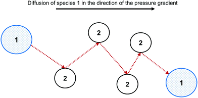
The Maxwell–Stefan (MS) model is developed from the kinetic theory of gases, by assuming that the force acting on an individual particle is in equilibrium with the resistance to fluid motion due to collisions with other species. Fig. 1 shows the MS model of diffusion for species 1 through species 2.There is extensive experimental evidence showing that the MS model is accurate for multicomponent, dilute gases.5,13 For a gas, the pressure gradient can be related to the chemical potential gradient, ∇μ. The MS model with a ∇μ driving force is:14
 | (1) |
For an n component system, ∇μi is related to the activity coefficient, γi, by:
 | (2) |
| J = −Ct[B]−1[Γ][∇x] | (3) |
 | (4) |
2.2 Fick's law
Fick's law proposes a linear dependence between the diffusion flux and the concentration gradient based upon experimental observations; it is not a theoretical development like the MS model. The generalised Fick's law for an n component system is written as:5| J = −Ct[D][∇x] | (5) |
2.3 Estimating ideal mobility coefficients
Since both Fick's law and the MS model describe the same physical process, they are related. Comparing eqn (3) and (5), the [D] predicted by MS model is:| [D] = [B]−1[Γ] | (6) |
This shows that the mutual diffusivities obtained from the MS model are composed of two distinct parts, namely hydrodynamic ([B]−1) and thermodynamic ([Γ]) influences. [D] can be obtained experimentally, as it is related to the concentration gradient. Therefore the MS model's accuracy can be determined by comparing its predicted [D] to that experimentally measured. However, Đij is not accessible by experiments and unlike gases, there is no universal kinetic theory for liquids that allows Đij to be predicted.5 Hence eqn (6) has been assumed to be correct and Đij have been calculated using [Γ] and the measured [D].
Due to both experimental and simulation difficulties, numerous semi-empirical relationships for predicting Đij have been developed. However, all these models are based on the assumption that the MS model is correct for liquid systems, which need not be the case. The two foremost means to estimate Đij are the Darken and Vignes models.
The Vignes equation is a logarithmic interpolation that only requires the infinite dilution values,15 whilst the Darken model is a linear interpolation.16,17
In previous work using pulsed gradient stimulated echo nuclear magnetic resonance (PGSTE-NMR) of the nearly ideal ternary system of methanol/butan-1-ol/propan-1-ol,18 we have shown that the multicomponent Darken model of Liu et al.8 is more accurate than that of Krishna and van Baten.7 However, the average error for the system was 26%. This large error is primarily a result of large errors at low compositions, where the system was modelled as ideal, and erroneous mutual diffusion data, the latter being prone to high errors due to the challenges associated with mutual diffusion in ternary systems. The multicomponent Darken mobility model is:8
 | (7) |
 | (8) |
The Vignes model is an empirical model.19 Since the objective of this paper is to compare the MS model and the dynamic fluctuation model for a ternary system, and due to there being a physical basis for the Darken model, eqn (7) will be used to estimate the ideal mobility. It is stressed that this work does not set out to assess the accuracy and the validity of the Darken model relative to the Vignes model.
2.4 Dynamic concentration fluctuation model
For binary mixtures, the MS model predicts a linear relationship between D and Γ: | (9) |
However, this is not experimentally observed for hexane/nitrobenzene as the consulate point is approached and for numerous other non-ideal binary systems.9–12
Previous work on binary systems has demonstrated that a model based on critical point scaling laws20 successfully predicts mutual diffusion in non-ideal binary mixtures, which is given by:
 | (10) |
![[D with combining circumflex]](https://www.rsc.org/images/entities/i_char_0044_0302.gif) ij is the ideal mobility between species i–j and α is a parameter from dynamic scaling theory.21 The parameter α is a system independent constant and is taken to be around two-thirds.5,22,23 The parameter α accounts for dynamic concentration fluctuations within the system. These occur because the driving force for the removal of these fluctuations is ∇μi, which tends to zero at the critical point. Hence, the processes removing such fluctuations become slow and the fluctuations become important in determining the physical properties of the mixture. At any point in a mixture with significant concentration fluctuations a diffusing species may experience a concentration either a little higher or a little lower than the mean concentration; the result will be that locally the thermodynamic correction factor is higher than that which would be expected from the mean concentration.24 This provides a theoretical explanation as to why α < 1, hence the non-linear dependence.
ij is the ideal mobility between species i–j and α is a parameter from dynamic scaling theory.21 The parameter α is a system independent constant and is taken to be around two-thirds.5,22,23 The parameter α accounts for dynamic concentration fluctuations within the system. These occur because the driving force for the removal of these fluctuations is ∇μi, which tends to zero at the critical point. Hence, the processes removing such fluctuations become slow and the fluctuations become important in determining the physical properties of the mixture. At any point in a mixture with significant concentration fluctuations a diffusing species may experience a concentration either a little higher or a little lower than the mean concentration; the result will be that locally the thermodynamic correction factor is higher than that which would be expected from the mean concentration.24 This provides a theoretical explanation as to why α < 1, hence the non-linear dependence.
Further work showed that the dynamic fluctuation model, with α = 0.64, was accurate in predicting the diffusivities of 14 non-ideal binary liquid mixtures, systems which exhibited both positive and negative deviations from Raoult's law and were far away from the consulate point.10,11 This provides further evidence that the MS model inaccurately accounts for the ∇μi driving force.
An explanation for the MS model's failure to accurately describe diffusion in highly non-ideal liquid mixtures is that the intermolecular forces become significant in such systems. These forces may result in clusters forming, with clusters and individual particles transported in the diffusion process,12 rather than the single spherical particles undergoing random elastic collisions proposed by the kinetic theory of gases, as is modelled in the MS model.5 Therefore, the extension of the MS model from dilute gases to highly non-ideal liquid systems does not have a strong theoretical foundation. The difference between the MS model and the underlying diffusion of highly non-ideal systems is shown in Fig. 2.
The success of the binary dynamic fluctuation model suggests that for a highly non-ideal ternary system a scaling power adjustment is required on Γ. [B]'s dependence on Đij, eqn (4) and (7), is expected to remain unchanged, as the dynamic fluctuation model only adjusts Γ due to concentration fluctuations; hence, the hydrodynamic influence is unaffected. However, for the dynamic fluctuation model Đ is replaced by ![[D with combining circumflex]](https://www.rsc.org/images/entities/i_char_0044_0302.gif) , the ideal mobility, with the only difference between these two coefficients being their physical interpretation in that
, the ideal mobility, with the only difference between these two coefficients being their physical interpretation in that ![[D with combining circumflex]](https://www.rsc.org/images/entities/i_char_0044_0302.gif) is an ideal mobility term whilst Đ is an inverse drag coefficient.
is an ideal mobility term whilst Đ is an inverse drag coefficient.
Modelling the mutual diffusion of a ternary system faces an additional complexity, as the entire system is a matrix and raising the matrix Γ to a fractional power cannot be done elementwise. Raising a matrix to a fractional power requires diagonalisation; a derivation is provided in the Appendix for the interested reader. Using matrix diagonalisation, the ternary dynamic fluctuation model becomes:
| [D] = [B]−1[Γ]α = [B]−1VΛαV−1 | (11) |
2.5 Local composition dynamic fluctuation model
An implicit assumption in the Darken model, eqn (7), is that![[D with combining circumflex]](https://www.rsc.org/images/entities/i_char_0044_0302.gif) can be determined from the measured self-diffusivities, D*, of single molecules. If, however, species’ motion is highly correlated due to strong association, this assumption is physically inconsistent. This is because the measured motion of a labelled molecule is accompanied by the motion of one or more unlabelled molecules. This problem can be overcome by using the local composition in the Darken model rather than the bulk composition.23
can be determined from the measured self-diffusivities, D*, of single molecules. If, however, species’ motion is highly correlated due to strong association, this assumption is physically inconsistent. This is because the measured motion of a labelled molecule is accompanied by the motion of one or more unlabelled molecules. This problem can be overcome by using the local composition in the Darken model rather than the bulk composition.23
The local composition form of the dynamic fluctuation model accurately predicts the mutual diffusion coefficients of both associating and non-associating species for binary systems.23 The applicability of the model to a wide variety of thermodynamic systems suggests that the dynamic fluctuation model has a strong predictive capacity. Indeed, such a model has also been recently tested and assessed by Guevara-Carrion et al.25 in a recently published work on mutual diffusion in binary mixtures, who concluded that this model was the most accurate predictive tool for mutual diffusion in binary systems.
Based on the success of using local mole fractions to account for association in binary systems,23 the local mole fraction model is extended to ternary systems. For the general multicomponent system, the NRTL (Non Random Two Liquid) model relates the local mole fraction of molecule j and k in the immediate neighbourhood of molecule i.26 To account for molecular association, the mole fraction of a component in its own immediate vicinity, xii, replaces its bulk mole fraction xi in the Darken mobility model, eqn (7), to yield:
 | (12) |
This impact on the ideal mobility only changes the hydrodynamic influence. The hydrodynamic influence for local composition, B*, is:
 | (13) |
The dynamic concentration fluctuation model using local compositions to account for molecular association is thus:
| [D] = [B*]−1[Γ]α = [B*]−1VΛαV−1 | (14) |
3. Experimental
Approaching the two-phase region of a partially miscible system will result in maximally non-ideal diffusion, and is hence the best means to identify the appropriate form of the thermodynamic correction factor. To test the ternary diffusion models across a wide-range of non-idealities, the coexistence curve was approached from the most ideal binary subsystem, toluene/n-decane.27 This pathway results in the ideality of the system continuously decreasing. Eight sample points were evaluated, as seen in Fig. 3.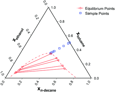 | ||
| Fig. 3 Ternary phase diagram of ethanol (1)/toluene (2)/n-decane (3) at 25 °C28,29 with the sampling points. The relative toluene/n-decane composition was kept constant with a molar ratio equal to one. | ||
3.1 Thermodynamic data
The ternary system ethanol (1)/toluene (2)/n-decane (3) is a partially miscible system at 25 °C, and has phase equilibrium data available.28 The thermodynamically consistent NRTL parameters for the system are presented in Table 1.29 These values were used to determine Γ, the thermodynamic correction factor, in the diffusion model.| i–j | τ ij | τ ji | ε ij |
|---|---|---|---|
| 1–2 | 2.091 ± 0.008 | 1.808 ± 0.014 | 0.470 ± — |
| 1–3 | 2.955 ± 0.004 | 2.253 ± 0.014 | 0.415 ± 0.0002 |
| 2–3 | 0.567 ± 0.006 | 2.051 ± 0.001 | 0.517 ± 0.002 |
3.2 Self-diffusion measurements
To undertake the ideal mobility analysis, D* measurements are required. The pulsed gradient stimulated echo nuclear magnetic resonance (PGSTE-NMR) method allows D* to be measured as a function of a species’ NMR signal decay.30 The details of the method have been reported elsewhere.9,24,31All NMR experiments were performed at a temperature of 298 K on a Bruker DMX 300 operating at a 1H frequency of 300.13 MHz. The NMR diffusion experiments were carried out using a diffusion probe capable of producing magnetic field gradient pulses up to 11.76 T m−1 in the z-direction. The duration of the 90° pulse of the 1H nuclei was 4.8 μs. A Bruker Variable Temperature unit, BVT 3000, was used to set the required temperature.
Self-diffusion measurements of the ethanol (1)/toluene (2)/n-decane (3) mixtures were conducted using the PGSTE pulse sequence.32 Measurements were performed by holding the gradient pulse duration (δ) constant and varying the gradient strength (g). The observation time (Δ) was set to 50 ms. All NMR spectra were referenced to bulk liquid TMS.
3.3 Mutual diffusion measurements
Mutual diffusion measurements were performed in a lab-scale equipment, constituted by a peristaltic pump, by which a solution of ethanol (1)/toluene (2)/n-decane (3) is flowing at a fixed flow-rate in a 20 m length capillary bore, characterised by an internal radius of r = 3.945 × 10⁻⁴ m. The pipe is set in a thermostatic bath working at 25 °C. The outlet flow is sent to a RI Detector (Knauer RI Detector K-2301) with a sensitivity of 3 × 10⁻⁸ RIU and a noise of ±1.5 × 10⁻⁸ RIU. The collected data were interpreted by applying the analytical solution of the laminar flow model reported in eqn (15) and (16).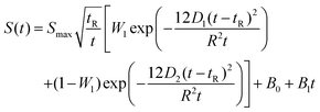 | (15) |
 | (16) |
D 1 and D2 represent the eigenvalues of the function, while W1 is the weight of the first peak function. α1 is the fraction of the initial refractive index contributed by solute 1, defined as in eqn (17).
 | (17) |
The eigenvalues are weighted through a linear correlation; a and b are the related parameters. D1, D2, a and b, were obtained by parameter estimation analysis on the collected experimental data. In particular, the objective function written as in eqn (18) was minimised by using the “particleswarm” algorithm implemented in MATLAB libraries.33
 | (18) |
The mutual diffusion coefficients were finally calculated as in eqn (19)–(22).
 | (19) |
 | (20) |
 | (21) |
 | (22) |
4. Results and discussion
4.1 Self-diffusion measurements
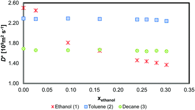
The self-diffusion measurements from the PGSTE-NMR experiments for the three components are shown below in Fig. 4. The values are reported for different ethanol mole fractions whilst the toluene/n-decane molar ratio is kept equal to one.The toluene and n-decane D* values only vary slightly over the composition range. However, Dethanol* at ethanol mole fractions less than 0.05 is substantially higher than that at ethanol mole fractions greater than 0.10. This suggests that ethanol undergoes strong molecular association at ethanol mole fractions above about 0.10. Above this mole fraction, Dethanol* decreases approximately linearly with increasing mole fraction.
The self-diffusion measurements are not at precisely the same mole fractions as the mutual diffusion mole fractions due to experimental difficulties involved in the measurements. To overcome this, a linear interpolation was used for D* of all the components. For ethanol, the linear interpolation was conducted in two separate sections, namely for xethanol < 0.10 and xethanol > 0.10.
4.2 Ternary mutual diffusion results
A comparison of the experimental mutual diffusion data and the results from the Maxwell–Stefan model and dynamic fluctuation model, eqn (11), with α = 0.64 is provided in Fig. 5. Both models are a poor approximation for D22 and D21 at all the experimental points investigated. However, the most notable difference between the models is for D22.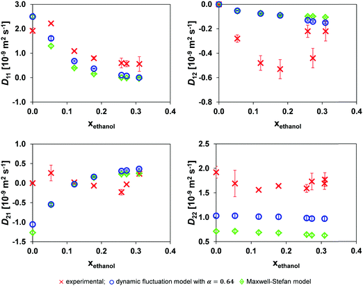 | ||
| Fig. 5 Comparison of the mutual diffusion data for ethanol (1)/toluene (2)/n-decane (3) at 25 °C using the dynamic fluctuation model, eqn (11) with α = 0.64, and the traditional Maxwell–Stefan model against experimental data. | ||
Considering the small variation in D* for toluene and n-decane over the composition range of interest and Dethanol* being almost linearly related to the ethanol mole fraction system for xethanol > 0.10, Fig. 4, there is only limited source of uncertainty from the hydrodynamic term in both the MS, eqn (6), and dynamic fluctuation models, eqn (11). Therefore, the source of the discrepancy in the predicted D22 and D21 from both models must lie either in the accuracy of the thermodynamic data or in the form of the models.
It is reasonable to expect the difference between the experimental data and the two models to be smallest at the lowest xethanol as this corresponds to a more thermodynamically ideal system. However, the ternary thermodynamic model was obtained from regressing the LLE (Liquid Liquid Equilibrium) coexistence curve. Therefore, as one moves further away from the coexistence curve, the ternary thermodynamic parameters become an extrapolation, although this influence is offset by the system becoming more ideal. Furthermore, in general the regressed ternary system parameters are unable to accurately model the binary subsystems VLE (Vapour Liquid Equilibrium).34 However, as one proceeds to the coexistence curve with increasing xethanol, as shown in Fig. 3, the ternary thermodynamic parameters are a more accurate representation of the system, in particular, at xethanol = 0.309 when the system is close to the coexistence curve.
Nevertheless, eqn (11) is an improvement over the traditional MS model for the entire composition range when considering D22 in Fig. 5. The absolute error of the models compared to the experimental data is provided in Table 2. The table clearly shows that the dynamic fluctuation model, eqn (11) with α = 0.64, is an improvement over the conventional MS model, eqn (6), except for D21 for which the absolute improvement of the MS formulation is marginal. Consequently, it is reasonable to claim that the dynamic fluctuation model with α = 0.64 is an improvement over the conventional MS model.
| Model | D 11 | D 12 | D 21 | D 22 |
|---|---|---|---|---|
| Eqn (11) | 0.512 | 0.269 | 0.442 | 0.710 |
| MS | 0.659 | 0.279 | 0.431 | 1.038 |
The results when using the local mole fraction for both the MS and dynamic concentration fluctuation models are shown in Fig. 6. As expected from its success in the binary systems, the local composition model provides improved performance.
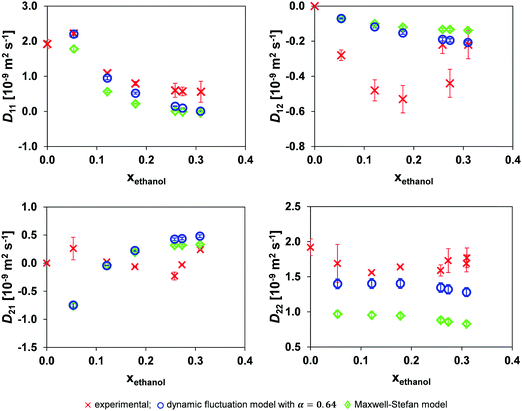 | ||
| Fig. 6 Comparison of the mutual diffusion data for ethanol (1)/toluene (2)/n-decane (3) at 25 °C using the local mole fraction in both the dynamic fluctuation model, eqn (14) with α = 0.64, and the traditional Maxwell–Stefan model against experimental data. | ||
Comparing Tables 2 and 3 one sees that the use of the local mole fraction model gives a noticeable improvement in the accuracy of both models. The reason for this is that strong molecular self-association of a polar species is expected when it is mixed with a non-polar one. This requires modification of the average molecular mobility; for example; if a species is dimerised, the self-diffusivity of the dimerised species should be doubled in the form of doubling the tracer diffusivity of the dimerised species.10 In this system, ethanol is expected to undergo molecular association, and this is consistent with the step change in Dethanol* at xethanol ∼ 0.10, Fig. 4. The use of a local mole fraction provides an a priori tool to account for the influence of cluster formation on the molecular mobility.23
| Model | D 11 | D 12 | D 21 | D 22 |
|---|---|---|---|---|
| Eqn (14) | 0.324 | 0.291 | 0.443 | 0.309 |
| MS | 0.557 | 0.306 | 0.378 | 0.761 |
Fig. 7 shows the change in both the absolute diagonal and total error between the experimental mutual diffusion data and that of the dynamic concentration fluctuation model for varying values of α. Clearly, as one decreases the value α from 1 through to ∼0.40, both the total and the diagonal error decrease. However, decreasing α from 0.50 to 0.40 sees a negligible change in the model prediction, as the error terms remain roughly constant. An α below 0.40 implies a reduction of the diffusion prediction accuracy. Therefore, the optimum α is in the range of 0.40 to 0.60. This result is similar to that of binary systems, which also have an optimum α of 0.40 to 0.80.10,11 This suggests that the scaling factor α is thus consistent with the theoretical scaling laws theory scaling factor of ∼0.64.
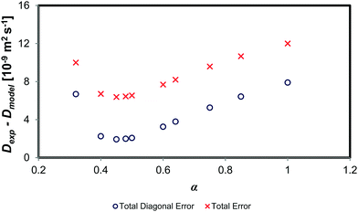 | ||
| Fig. 7 Comparison of absolute error between experimental data and the of the dynamic concentration fluctuation model with varying values of α. | ||
Fig. 8 shows the result of the application of the dynamic concentration fluctuation model using local mole fraction with the optimal α of 0.45. There is a distinct improvement in the accuracy of the model, with this being most prominent for D22. Table 4 shows that the local mole fraction model is approximately an order of magnitude more accurate than the traditional MS model.
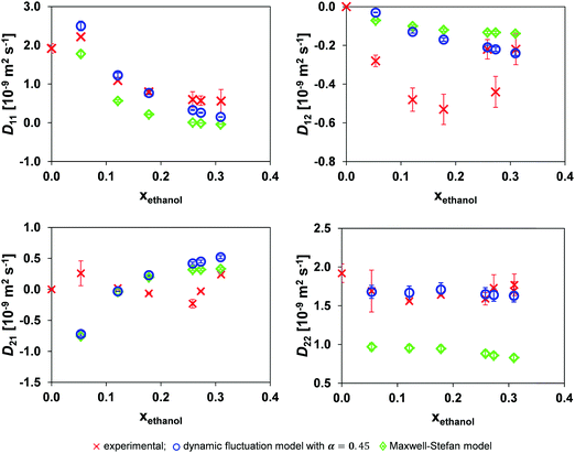 | ||
| Fig. 8 Comparison of the mutual diffusion data for ethanol (1)/toluene (2)/n-decane (3) at 25 °C using local mole fraction in both the dynamic fluctuation model, eqn (14) with α = 0.45, and the traditional Maxwell–Stefan model against experimental data. | ||
| Model | D 11 | D 12 | D 21 | D 22 |
|---|---|---|---|---|
| Eqn (14) | 0.233 | 0.283 | 0.459 | 0.089 |
| MS | 0.557 | 0.306 | 0.378 | 0.761 |
5. Conclusion and recommendations
The dynamic fluctuation model, which uses the scaling factor α to reduce the non-ideal thermodynamic impact based on scaling theory, was extended to ternary systems. The developed model and the most common model currently in use, the Maxwell–Stefan model, were compared to experimental mutual diffusion data for the partially miscible system ethanol/toluene/n-decane. The analysis showed that the Maxwell–Stefan formulation inaccurately accounts for the thermodynamic influence on diffusion, the same conclusion as that for binary systems.9–11 The inaccuracy of the Maxwell–Stefan model for both binary and ternary systems suggests that the key assumptions in its derivation, which are rooted in the kinetic theory of gases, are invalid for highly non-ideal liquid systems.Considering the shortcomings of the Maxwell–Stefan formulation, molecular dynamic simulations are not an entirely appropriate means for further diffusion model validation. The developed model improves prediction of mutual diffusion; in particular, using such model with local mole fractions, to account for self-association of ethanol, substantially improved the match between predicted and measured diffusion coefficients. Thus, the model which best predicted experimental results was one incorporating local compositions into the hydrodynamic term, as well as a modulation of the thermodynamic correction factor due to dynamic concentration fluctuations, eqn (14). An interesting result is that optimum α for the ternary system investigated is approximately 0.45. This is similar to the optimum α of 0.40 to 0.80 for a range of binary systems previously investigated.10,11 This suggests that the α scaling factor is uniform.
We note that further work is required to test the accuracy of the ternary dynamic fluctuation model, and determine whether or not the scaling factor α is uniform, as was the case for binary systems.10,11 To reduce the uncertainties in thermodynamic modelling and thus improve model discrimination, ternary VLE data must be obtained for the chosen sample points at the temperature of interest. Ternary VLE data is preferred over LLE data, as VLE data can be obtained for partially miscible systems at sample points outside the two-phase coexistence region. Thus, more VLE data would allow the thermodynamics to be accurately modelled within the region of interest; it would no longer be an extrapolation from the two-phase coexistence region, as is the case with using thermodynamic parameters regressed from LLE data obtaining a high discrepancy between the experimental data and the model extrapolation.
It is important to note that ternary systems are complex to analyse, both in terms of experimental measurements of mutual diffusion and determination of accurate thermodynamic data and this is perhaps the reason why few systems have so far been investigated. However, as shown in this work, the use of the dynamic concentration fluctuation diffusion model with local compositions for binary systems23 and its extension to the ternary system in this work warrant further investigation on other ternary systems.
Conflicts of interest
There are no conflicts to declare.A. Appendix
Fractional power of matrix derivation
Let us assume that the square matrix A can be diagonalised via eigenvalue decomposition and written as:| A = VΛV−1 | (A.1) |
| A2 = AA = VΛV−1VΛV−1 = VΛ2V−1 | (A.2) |
| Aα = VΛαV−1 | (A.3) |
Since Λ is a diagonal matrix, it follows that:
 | (A.4) |
For a general real-valued square matrix, the eigenvalues can be negative or complex. In either of these cases, fractional powers of the matrix might feature complex entries. In the case of the diffusion matrix Γ raised to α:
| Γα = VΛαV−1 | (A.5) |
The ternary dynamic fluctuation model becomes:
| [D] = [B]−1[Γ]α = [B]−1VΛαV−1 | (A.6) |
The ternary dynamic fluctuation model just requires the eigen decomposition of the thermodynamic matrix, Γ.
Ternary local mole fraction model derivation
For the general multicomponent system, the NRTL (Non Random Two Liquid) model relates the local mole fraction of molecule j and k in the immediate neighbourhood of molecule i.26 To account for molecular association, the mole fraction of a component in its own immediate vicinity, xii, replaces its bulk mole fraction xi in the Darken mobility model, eqn (7), to yield: | (A.7) |
For each bulk composition for a ternary system, there are three local mole fraction relationships, eqn (A.7), and one local mole fraction balance, eqn (A.8). This provides a set of four equations that must be implicitly solved to yield the local mole fractions for each ternary composition.
 | (A.8) |
Nomenclature
| a | Eigenvalues weight parameter (—) |
| b | Eigenvalues weight parameter (—) |
| B 0 | Baseline correction constant (mV) |
| B 1 | Baseline correction constant (mV) |
| B | Hydrodynamic diffusion influence (m2 s−1) |
| B* | Local composition hydrodynamic diffusion influence (m2 s−1) |
| C i | Concentration of component i (mol m−3) |
| C t | Total molar concentration (mol m−3) |
| D ii | Main diffusion coefficient of component i (m2 s−1) |
| D ij | Cross diffusion coefficient of component i under the j concentration gradient (m2 s−1) |
| D j | Eigenvalues (m2 s−1) |
| Đ ij | Maxwell–Stefan diffusion coefficient between i–j (m2 s−1) |
| D i * | Self diffusion coefficient of i (m2 s−1) |
![[D with combining circumflex]](https://www.rsc.org/images/entities/i_char_0044_0302.gif) ij
ij
| Ideal mobility between i–j (m2 s−1) |
| f(x) | Objective function (—) |
| f I i | Fugacity of i in phase I (—) |
| G | Gibbs energy (J mol−1 K−1) |
| g ij | Energies of interaction between i–j pair of molecules (J mol−1 K−1) |
| J i | Molar flux of i (mol m−2 s−1) |
| k | Detector constant (mV) |
| M | Total tie-lines (—) |
| N | Number of collected experimental data (—) |
| P tot | Total pressure (bar) |
| P vap i | Vapour pressure of i (bar) |
| r | Pipe inner radius (m) |
| R | Universal gas constant (J mol−1 K−1) |
| R i | Molar refractivities (m3 mol−1) |
| S | Detector signal (mV) |
| S calc | Calculated detector signal (mV) |
| S exp | Experimental detector signal (mV) |
| t | Time (s) |
| t R | Retention time (s) |
| T | System temperature (K) |
| T c | Consulate temperature (K) |
| w i | Mass fraction of i (—) |
| W 1 | Eigenvalues weight (—) |
| x i | Mole fraction of i (—) |
![[x with combining circumflex]](https://www.rsc.org/images/entities/i_char_0078_0302.gif) i
i
| Activity coefficient model calculated mole fraction of i (—) |
Greek letters
| α | Dynamic fluctuation parameter (—) |
| α 1 | Fraction of the initial refractive index (—) |
| ΔCi | Concentration difference between the stream and the pulse of component i (mol m−3) |
| ε ij | NRTL non-randomness parameter between i–j (—) |
| μ i | Chemical potential energy of i (J mol−1 K−1) |
| Γ | Thermodynamic correction factor (—) |
| γ i | Activity coefficient of i (—) |
| τ | UNIQUAC i–j interaction parameter (—) |
Acknowledgements
Carmine D’Agostino is grateful to Wolfson College, Cambridge, for supporting his research activities. Tariq Allie-Ebrahim is a Commonwealth Scholar. We would also like to acknowledge Prof. Lynn Gladden for the access to the NMR facilities used for the experimental measurements.References
- R. Brodkey and H. Hershey, Transport Phenomena: A Unified Approach, Brodkey Publishing, Ohio, 2003, pp. 711–788 Search PubMed.
- A. Bardow, E. Kriesten, M. Voda, F. Casanova, B. Blumich and W. Marquardt, Prediction of multicomponent mutual diffusion in liquids: Model discrimination using NMR, Fluid Phase Equilib., 2009, 278(1), 27–35 CrossRef.
- A. Bardow, V. Göke, H. Koß and W. Marquardt, Ternary diffusivities by model-based analysis of Raman spectroscopy measurements, AIChE J., 2006, 52(12), 4004–4015 CrossRef.
- I. van de Ven-Lucassen, M. Kemmere and P. Kerkhof, Complications in the Use of the Taylor Dispersion Method for Ternary Diffusion Measurements: Methanol + Acetone + Water Mixtures, J. Solution Chem., 1997, 26(12), 1145–1167 CrossRef.
- R. Krishna and J. Wesselingh, The Maxwell Stefan approach to mass transfer, Chem. Eng. Sci., 1997, 52(6), 861–911 CrossRef.
- R. Krishna, Serpentine diffusion trajectories and the Ouzo effect in partially miscible ternary liquid mixtures, Phys. Chem. Chem. Phys., 2015, 17(41), 27428–27436 RSC.
- R. Krishna and J. van Baten, The Darken relation for multicomponent diffusion in liquid mixtures of linear alkanes: an investigation using molecular dynamics (MD) simulations, Ind. Eng. Chem. Res., 2005, 44(17), 6939–6947 CrossRef.
- X. Liu, T. Vlugt and A. Bardow, Maxwell–Stefan diffusivities in liquid mixtures: Using molecular dynamics for testing model predictions, Fluid Phase Equilib., 2011, 301(1), 110–117 CrossRef.
- C. D'Agostino, M. Mantle, L. Gladden and G. Moggridge, Prediction of binary diffusion coefficients in non-ideal mixtures from NMR data: hexane–nitrobenzene near its consolute point, Chem. Eng. Sci., 2011, 66(17), 3898–3906 CrossRef.
- G. Moggdridge, Prediction of the mutual diffusivity in binary liquid mixtures containing one dimerising species, from the tracer diffusion coefficients, Chem. Eng. Sci., 2012, 76, 199–205 CrossRef.
- G. Moggridge, Prediction of the mutual diffusivity in binary non-ideal liquid mixtures from the tracer diffusion coefficients, Chem. Eng. Sci., 2012, 71, 226–238 CrossRef.
- E. Cussler, Cluster diffusion in liquids, AIChE J., 1980, 26(1), 43–51 CrossRef.
- E. Cussler, Diffusion: mass transfer in fluid systems, Cambridge University Press, Cambridge, 2009 Search PubMed.
- J. Wesselingh and R. Krishna, Mass Transfer in Multicomponent Mixtures, Delft University Press, 2000 Search PubMed.
- H. Kooijman and R. Taylor, Estimation of diffusion coefficients in multicomponent liquid systems, Ind. Eng. Chem. Res., 1991, 30(6), 1217–1222 CrossRef.
- L. Darken, Diffusion, mobility and their interrelation through free energy in binary, Am. Inst. Min., Metall., Pet. Eng., 1948, 175, 184–201 Search PubMed.
- S. Rehfeldt and J. Stichmair, Measurement and prediction of multicomponent diffusion coefficients in four ternary liquid systems, Fluid Phase Equilib., 2010, 290, 1–14 CrossRef.
- T. Allie-Ebrahim, Q. Zhu, P. Brauer, G. Moggridge and C. D'Agostino, Maxwell–Stefan diffusion coefficient estimation for ternary systems: an ideal ternary alcohol system, Phys. Chem. Chem. Phys., 2017, 19, 16071–16077 RSC.
- R. Taylor and R. Krishna, Multicomponent mass transfer, Wiley, New York, 1993 Search PubMed.
- W. Clark and R. Rowley, The mutual diffusion coefficient of methanol n-hexane, AIChE J., 1986, 32(7), 1125–1131 CrossRef.
- S. De, Y. Shapir and E. Chimowitz, Scaling of self and Fickian diffusion coefficients in the critical region, Chem. Eng. Sci., 2001, 56, 5003–5010 CrossRef.
- G. Wu, M. Fiebig and A. Leipertz, Local composition based Maswell–Stefan diffusivity model for binary liquid systems, Ind. Eng. Chem., 2013, 52, 10845–10852 CrossRef.
- Q. Zhu, G. Moggridge and C. D'Agostino, A local composition model for the prediction of mutual diffusion coefficients in binary liquid mixtures from tracer diffusion coefficients, Chem. Eng. Sci., 2015, 132, 250–258 CrossRef.
- C. D'Agostino, R. Harris, A. Abbott, L. Gladden and M. Mantle, Molecular motion and ion diffusion in choline chloride based deep eutectic solvents studied by 1H pulsed field gradient NMR spectroscopy, Phys. Chem. Chem. Phys., 2011, 13(48), 21383–21391 RSC.
- G. Guevara-Carrion, T. Janzen, Y. Mauricio Muñoz-Muñoz and J. Vrabeca, Mutual diffusion of binary liquid mixtures containing methanol, ethanol, acetone, benzene, cyclohexane, toluene, and carbon tetrachloride, J. Chem. Phys., 2016, 144, 124501 CrossRef PubMed.
- H. Renon and J. Prausnitz, Local Compositions in Thermodynamic Excess Functions for Liquid Mixtures, AIChE J., 1968, 14(1), 135–144 CrossRef.
- M. Goral, Vapour–liquid equilibria in non-polar mixtures. III. Binary mixtures of alkylbenzenes and n-alkanes at 313.15 K, Fluid Phase Equilib., 1994, 102(2), 275–286 CrossRef.
- M. Mohsen-Nia, Ternary liquid–liquid equilibria for mixtures of (ethanol + toluene + n-decane), Phys. Chem. Liq., 2007, 45(5), 541–548 CrossRef.
- T. Allie-Ebrahim, Q. Zhu, G. Moggridge and C. D'Agostino, Liquid–liquid equilibrium for the ternary system ethanol/toluene/decane, Phys. Chem. Liq., 2016, 55(5), 669–673 CrossRef.
- E. Stejskal and J. Tanner, Spin Diffusion Measurements: Spin Echoes in the Presence of a Time-Dependent Field Gradient, J. Chem. Phys., 1965, 42(1), 288–292 CrossRef.
- C. D'Agostino, L. Gladden, M. Mantle, A. Abbott, E. Ahmed, A. Al-Murshedi and R. Harris, Molecular and ionic diffusion in aqueous – deep eutectic solvent mixtures: probing inter-molecular interactions using PFG NMR, Phys. Chem. Chem. Phys., 2015, 17(23), 15297–15304 RSC.
- J. Tanner, Use of the Stimulated Echo in NMR Diffusion Studies, J. Chem. Phys., 1970, 52(5), 2523–2526 CrossRef.
- V. Russo, O. Ortona, R. Tesser, L. Paduano and M. Di Serio, On the importance of choosing the best minimization algorithm for the determination of ternary diffusion coefficients by the Taylor Dispersion method, ACS Omega, 2017, 2(5), 2945–2952 CrossRef.
- Z. Li, K. Smith, K. Mumford, Y. Wang and G. Stevens, Regression of NRTL parameters from ternary liquid–liquid equilibria using particle swarm optimization and discussions, Fluid Phase Equilib., 2015, 398, 36–45 CrossRef.
| This journal is © the Owner Societies 2018 |

