DOI:
10.1039/C6SM01853J
(Paper)
Soft Matter, 2017,
13, 328-344
Tug-of-war between two elastically coupled molecular motors: a case study on force generation and force balance
Received
11th August 2016
, Accepted 17th November 2016
First published on 17th November 2016
Abstract
Intracellular transport is performed by molecular motors that pull cargos along cytoskeletal filaments. Many cellular cargos are observed to move bidirectionally, with fast transport in both directions. This behaviour can be understood as a stochastic tug-of-war between two teams of antagonistic motors. The first theoretical model for such a tug-of-war, the Müller–Klumpp–Lipowsky (MKL) model, was based on two simplifying assumptions: (i) both motor teams move with the same velocity in the direction of the stronger team, and (ii) this velocity matching and the associated force balance arise immediately after the rebinding of an unbound motor to the filament. In this study, we extend the MKL model by including an elastic coupling between the antagonistic motors, and by allowing the motors to perform discrete motor steps. Each motor step changes the elastic interaction forces experienced by the motors. In order to elucidate the basic concepts of force balance and force fluctuations, we focus on the simplest case of two antagonistic motors, one kinesin against one dynein. We calculate the probability distribution for the spatial separation of the motors and the dependence of this distribution on the motors' unbinding rate. We also compute the probability distribution for the elastic interaction forces experienced by the motors, which determines the average elastic force 〈F〉 and the standard deviation of the force fluctuations around this average value. The average force 〈F〉 is found to decrease monotonically with increasing unbinding rate ε0. The behaviour of the MKL model is recovered in the limit of small ε0. In the opposite limit of large ε0, 〈F〉 is found to decay to zero as 1/ε0. Finally, we study the limiting case with ε0 = 0 for which we determine both the force statistics and the time needed to attain the steady state. Our theoretical predictions are accessible to experimental studies of in vitro systems consisting of two antagonistic motors attached to a synthetic scaffold or crosslinked via DNA hybridization.
1 Introduction
Intracellular cargos such as vesicles and organelles are transported by cytoskeletal motors.1 Conventional kinesin and cytoplasmic dynein represent two types of cytoskeletal motors that walk along microtubules in opposite directions.2,3 Many cargos are observed to perform a bidirectional movement on the microtubules with frequent reversals.4,5 This behaviour reflects the presence of two antagonistic motors, plus-end directed kinesin and minus-end directed dynein, on the same cargo. These motors try to pull the cargo in their preferred direction of motion, thereby performing a stochastic tug-of-war. The first theoretical model for such a stochastic tug-of-war was introduced by Müller, Klumpp, and Lipowsky (MKL)6–8 and corroborated by the observations of endosome transport in amoebae9 and fungi.10
The MKL model was based on two simplifying assumptions: (i) all motors move with the same velocity in the direction of the stronger team and (ii) this matching of the velocities sets in as soon as the cargo is pulled by motors from both teams. Thus, for two antagonistic motors, the MKL tug-of-war state is characterized by the following properties. When both motors are simultaneously bound to the filament, they experience mutual interaction forces which are of equal magnitude and opposite direction, in accordance with Newton's third law. The absolute value of this interaction force, the so-called cargo force Fca, is determined uniquely by the characteristic force–velocity relations of the motors and the condition of velocity-matching under this force.6,8 The cargo then moves with this generally low, but nonzero velocity vca in the direction of the stronger motor. In the special case of equally strong motors the cargo is in a stalled state with zero velocity.
In the MKL model, the motion of the motors is described in a coarse-grained manner, averaging over the discrete steps of the individual motors. Here, we extend this model by including these discrete steps, following the theoretical approach developed in ref. 11 and 12 for two identical motors that pull in the same direction. We consider two antagonistic motors which are coupled to their common cargo via two elastic linkers. We then use the force balance between the motors and the cargo to derive an effective elastic coupling between the two motors. With each step taken by one of the motors, the effective linker is either stretched or compressed and an elastic force is induced acting on both motors. The velocity-matching condition can therefore only be reached, in general, after the motors have taken multiple steps.
When the tug-of-war involves antagonistic motor teams consisting of several identical motors, the MKL model makes the additional assumption that the overall load acting on one team is shared equally by all motors in that team. This assumption has been previously criticized to represent a mean-field approximation because it ignores fluctuations in the load sharing.13–15 In order to examine the latter fluctuations, the authors in ref. 13–15 studied such antagonistic motor teams. In contrast to these previous studies, we focus here on the simplest case of two antagonistic motors for which load sharing does not play any role. On the one hand, the case of 1 + 1 motors is useful in order to elucidate the basic concepts of force balance and force fluctuations. In fact, as shown below, this case already implies a nontrivial force balance, with an average interaction force that depends strongly on the unbinding rate ε0 of the individual motors and decays to zero for large ε0. On the other hand, the study of the 1 + 1 motor system allows us to perform a detailed comparison between (i) the tug-of-war of two elastically coupled motors that perform discrete steps and (ii) the tug-of-war of two antagonistic motors as described by the MKL model.
The theoretical results described below can be scrutinized by experimental in vitro studies based on recently developed protocols16–20 to control the number of active motors on synthetic molecular scaffolds. Evidence for a tug-of-war mechanism between kinesin and dynein attached to such scaffolds was observed in ref. 19 and 20. Very recently, it has also been demonstrated that one can directly crosslink a single, fluo-labeled kinesin with a single, fluo-labeled dynein via DNA hybridization.21 For such two-motor constructs, one should be able to measure the probability distribution for the spatial separation of the two motors along the filament and, in this way, directly scrutinize the predictions of our theory. Furthermore, as shown below, the distribution for the motor–motor separation also determines the probability distribution for the elastic interaction forces and, thus, the average elastic force 〈F〉 between the motors.
This paper is organized as follows. First, we briefly review (i) the single motor description in Section 2.1, thereby introducing the single motor parameters used in our model, and (ii) the cargo force predicted by the MKL model in Section 2.2. Next, the force balance for a tug-of-war between two elastically coupled motors is considered and the associated state space for this process is defined in Section 2.3. We describe the system as a Markov process with (i) several transient states corresponding to different extensions of the effective elastic linker and (ii) two absorbing states defined by a single plus- or minus-end motor bound to the filament. The rates of the network are determined using single motor parameters characterising the stepping and unbinding behaviour. Section 3 reports the results on the steady state probability distributions of 2-motor runs with both motors attached to the filament, the average force experienced by the motors, as well as a detailed study of the limiting case of zero unbinding rates. In the latter case, both the force statistics and the time needed to reach the steady state are determined as a function of the elastic coupling strength.
2 Model
2.1 Single motor description
When a motor binds to the filament, it steps along the filament in a preferred direction. In the absence of an external force F, the motor moves with its zero-force forward velocity towards the preferred end of the filament. We use the convention that a resisting force acting as a load on the motor has a positive sign whereas an assisting force pulling the motor in its preferred stepping direction has a negative sign. This convention is used both for plus-directed and for minus-directed motors. With increasing load force, the motor velocity decreases until the force reaches the motor's stall force Fs at which the motor velocity vanishes. Experimental studies provide strong evidence that the kinesin-1 motor steps backwards for load forces F > Fs.22,23 The explicit form of the force–velocity relation for a single motor can be obtained from fits to experimental data or provided by piecewise linear relations as in previous theoretical studies, see e.g.ref. 6, 13 and 15 and Appendix A. Here, we will use a convenient parametrization of the force–velocity relation as introduced in ref. 11 which has the form| | 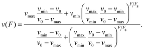 | (2.1) |
The parameters vmax and vmin determine the limits of v(F) for large negative and large positive values of F, respectively. The zero-force velocity v(F = 0) is given by the parameter v0. In the following, we use the force–velocity relation in eqn (2.1) for both motors. The parameters v0, vmax, vmin and Fs can be specified in order to obtain close approximations for experimentally determined force–velocity relations, e.g. as given in ref. 22 for kinesin-1 and in ref. 24 for cytoplasmic dynein.
Another single motor property that has been measured for kinesin as a function of load force22,23 is the forward-to-backward stepping ratio q which is defined as the number of forward steps divided by the number of backward steps as observed within a certain time interval. This ratio was found to depend exponentially on the load force and to be well fitted by22
| |  | (2.2) |
For dynein, the corresponding parameters have not been measured directly but the single motor data on yeast dynein in
ref. 25 and 26 provide the estimates
| | | q0 = 4 and Fs = 7 pN for dynein. | (2.3) |
We now use the force–velocity relationship v(F) and the forward-to-backward stepping ratio q(F) together with the step size ![[small script l]](https://www.rsc.org/images/entities/char_e146.gif) to define the forward stepping rate of a single motor by
to define the forward stepping rate of a single motor by
| |  | (2.4) |
and its backward stepping rate by
| |  | (2.5) |
which implies
α/
β =
q and
α −
β =
![[small script l]](https://www.rsc.org/images/entities/char_e146.gif) v
v.
11 The force-dependence of the two stepping rates
α and
β is illustrated in
Fig. 1 for yeast dynein. At the stall force
F =
Fs, the two stepping rates are equal, implying that forward and backward steps are equally likely. For
F >
Fs, backward steps are more likely than forward steps and both stepping rates decay monotonically with increasing force. For
F <
Fs, on the other hand, forward steps are more likely than backward steps but the individual stepping rates are nonmonotonic as a function of
F. In fact, the backward stepping rate
β for dynein exhibits a pronounced maximum at the load force
F = 3.21 pN, arising from the relatively small value
q0 = 4 of the forward-to-backward stepping ratio. For kinesin, on the other hand, which is characterized by a much larger value of
q0, no such maximum of
β is found.
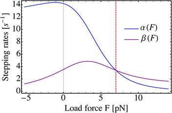 |
| | Fig. 1 Forward and backward stepping rates, α and β, as a function of load force F for yeast dynein. The rates are computed viaeqn (2.4) and (2.5) with the force–velocity relationship v(F) and the step ratio q(F) as given by eqn (2.1) and (2.2), using the single motor parameters in Table 1. The dashed vertical line (red) corresponds to the motor's stall force Fs = 7 pN. | |
A motor bound to a filament unbinds from this filament with a constant unbinding rate in the absence of external forces. We denote this zero-force unbinding rate of a single motor by ε0. When a force acts on the cargo, the motor-filament bond is more likely to break. Although the unbinding process is very complex on a molecular scale, it can be approximately described as an escape process of a particle in a potential well. According to Kramers' theory,27 the force-dependence of the motor's unbinding rate is then approximately exponential and given by
| | ε(F) = ε0![[thin space (1/6-em)]](https://www.rsc.org/images/entities/char_2009.gif) exp(|F|/Fd), exp(|F|/Fd), | (2.6) |
where
Fd is the detachment force, another force scale that characterizes each motor type. Here and below, the force
F represents the tangential force component acting parallel to the long axis of the filament, with the previously mentioned sign convention that
F is positive when it acts against the preferred stepping direction that the motor has in the absence of force. Note that
ε(
F) is taken to depend only on the absolute value |
F|, and not on the direction of the force which implies that resisting and assisting forces increase the unbinding rate by the same amount. This simplifying assumption is not crucial, however, because, as we will see below, assisting forces are almost never generated by a tug-of-war.
In the following, we use this single motor description for two different types of motors, kinesin and dynein, which represent the best studied examples for processive plus-end and minus-end directed motors. We will use the notation F±s and F±d for the stall and detachment forces of these two motor species. Our sign convention for F implies that both stall and detachment forces are positive. In addition, this convention also implies that a positive force acting on the plus-end directed motor points towards the minus end of the filament whereas a positive force acting on the minus-end directed motor points towards the filament's plus end. Furthermore, because of the opposite directionality, the force–velocity relationships v+(F) and v−(F) for the plus- and minus-directed motors have the form v+(F) = +v(F) and v−(F) = −v(F) with v(F) as in eqn (2.1).
2.2 Cargo force in the MKL model
Before we consider the tug-of-war between elastically coupled motors, we will first summarize the main properties of the tug-of-war in the MKL model which provides a useful reference process. As described in Appendix A, the latter process is characterized by instantaneous velocity matching between the different motors. The corresponding matching condition can be visualized by plotting the two force–velocity relations for the individual motors in the same (F,v)-diagram.8 The intersection point of these two relations provides the matching condition for the MKL tug-of-war as illustrated in Fig. 2 for the case in which the stall force F+s of the plus motor exceeds the stall force F−s of the minus motor.
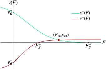 |
| | Fig. 2 Matching condition for the velocities of two antagonistic motors as used in the MKL tug-of-war model: force–velocity relations as given by eqn (2.1) for a plus (green) and a minus (red) motor with zero-force velocities v+0 > 0 and v−0 < 0. The intersection point (F, v) = (Fca, vca) of the two force–velocity relations defines the velocity-matched state in which both motors move with the same velocity vca and experience the same single motor force as provided by the cargo force F = Fca. In this example, the stall force F+s of the plus motor exceeds the stall force F−s of the minus motor which implies vca > 0, i.e. both the cargo and the two antagonistic motors move towards the plus end of the filament. | |
In general, the intersection point (F, v) = (Fca, vca) of the two force–velocity relations defines the velocity-matched state in which the cargo and the motors move with the same velocity vca and the two motors experience the same single motor force, namely the cargo force F = Fca. The cargo force is always positive because it is located between the stall forces F+s and F−s of the two motors, both of which are positive by definition. Thus, according to our sign convention for single motor forces, the cargo force acts as a resisting force on both motors: it represents the absolute value of the two opposing forces that the cargo exerts simultaneously onto the plus and onto the minus motor.
2.3 Elastic coupling between the motors
We now consider one kinesin and one dynein motor pulling on the same cargo particle via elastic linkers as illustrated in Fig. 3. We use the Cartesian coordinate x parallel to the filament to describe the positions of the motors and the cargo along this filament. The coordinate x is chosen to increase towards the plus end of the filament. Thus, each motor–cargo configuration is described by the positions xki, xdy, and xca with xdy < xca < xki. Furthermore, to discuss the elastic forces acting between the motors and the cargo, we will first define these forces with respect to the coordinate x which implies that we temporarily use a different sign convention for these interaction forces compared to the single motor forces. Thus, in the following paragraph, the elastic interaction forces are taken to be positive when they point towards the plus end of the filament and negative when they point towards the filament's negative end.
 |
| | Fig. 3 Different states (j) with j = 0, 1, m and n of two antagonistic motors corresponding to different extensions of the elastic linkers between the motors and the cargo. The kinesin motor (blue “heads”) and the dynein motor (green “wheels”) prefer to move towards the (+)- and (−)-end of the microtubule, respectively. In state (0), the motor linkers are relaxed and do not generate elastic forces. When the motors perform steps leading to a state (j) with j > 0, the spring becomes stretched and generates the elastic force Fj = jFK. As explained in the main text, the single motor forces Fki and Fdy acting on kinesin and dynein are defined in such a way that Newton's third law assumes the simple form Fj = Fki = Fdy. In state (1), for example, both the kinesin and the dynein motor experience the single motor force F1 = FK. In state (m), the force Fm = mFK ≃ F−s, i.e. it is comparable to the stall force F−s of the minus motor. At this stall force, the minus motor steps forward and backward with equal probability. In state (n), the force Fn is close to the stall force of the plus motor, which can now step forward and backward with (almost) equal probability. | |
Elastic forces between the cargo and the motors.
The linkers between the motors and the cargo are described by harmonic springs with spring constant κ and rest length L∥. The kinesin motor then exerts the force| | | Fki,ca = κ(xki − xca − L∥) | (2.7) |
onto the cargo. Likewise, the dynein motor exerts the force| | | Fdy,ca = −κ(xca − xdy − L∥) | (2.8) |
onto the cargo. We now assume that, for given positions xki and xdy, the elastic forces balance each other on timescales that are short compared to the timescales of the single motor transitions. This elastic force balance implies Fki,ca + Fdy,ca = 0 and xca = ½(xki + xdy). Eliminating the cargo position xca from the expressions in eqn (2.7) and (2.8), we obtain the forces| | | Fki,ca = ½κ(xki − xdy − 2L∥) = K(xki − xdy − L0) | (2.9) |
and| | | Fdy,ca = ½κ(xki − xdy − 2L∥) = −K(xki − xdy − L0), | (2.10) |
which depend only (i) on the coordinate difference xki − xdy of the two motor positions and (ii) on the effective spring parameters| | | K ≡ κ/2 and L0 = 2L∥. | (2.11) |
Introducing the combined spring extension| | | ΔL ≡ xki − xdy − L0, | (2.12) |
the force that the kinesin exerts on the dynein becomes| | | Fki,dy = Fki,ca = KΔL, | (2.13) |
while the force that the dynein exerts on the kinesin has the formas required by Newton's third law.
Identification with single motor forces.
In order to use the single motor description as described in the previous subsection, we now return to our original sign convention for the force F acting on a single motor. As a consequence, the single motor force is given by| | | F = Fki ≡ −Fdy,ki for kinesin, | (2.15) |
which is positive when the force Fdy,ki points towards the minus end of the filament, and by| | | F = Fdy ≡ Fki,dy for dynein, | (2.16) |
which is positive when the force Fki,dy points towards the filament's plus end. Newton's third law as given by Fki,dy = −Fdy,ki then assumes the simple form Fki = Fdy = F.
State space for tug-of-war with elastic coupling.
Kinesin and dynein have the same step size ![[small script l]](https://www.rsc.org/images/entities/char_e146.gif) ≃ 8 nm, see references in Table 1. We further assume that the motor pair can attain a relaxed state with ΔL = 0. It is then convenient to introduce the dimensionless spring extension
≃ 8 nm, see references in Table 1. We further assume that the motor pair can attain a relaxed state with ΔL = 0. It is then convenient to introduce the dimensionless spring extension| | j = ΔL/![[small script l]](https://www.rsc.org/images/entities/char_e146.gif) with −J ≤ j ≤ J, with −J ≤ j ≤ J, | (2.17) |
where j = J represents the maximal stretching and j = −J the maximal compression of the spring.
Table 1 Values of the parameters used for kinesin-1 and two types of dynein motors: the values for “strong” and “weak” dynein correspond to yeast and mammalian cells, respectively. A star superscript indicates a parameter for which we did not find experimental data in the literature; the corresponding parameter value was set equal to the experimentally deduced value of another type of motor. For the minimal and maximal velocities of both dynein motors in the force–velocity relationship (2.1) we used the estimated values vmin ≃ 0.12v0 and vmax ≃ 1.12v0, as indicated by the † symbol. For the parameters in this table the strain force is given by FK = κl/2 = 0.8 pN both for kinesin vs. strong dynein and for kinesin vs. weak dynein
| Parameter |
Kinesin-1 |
“Strong” dynein |
“Weak” dynein |
| Zero-force unbinding rate ε0 [s−1] |
135 |
1* |
136 |
| Stall force Fs [pN] |
722 |
724,26 |
1.137,38 |
| Detachment force Fd [pN] |
3.639 |
3.340 |
3.3* |
| Linker stiffness κ [pN nm−1] |
0.217 |
0.2* |
0.2* |
| Step size l [nm] |
817,22 |
825 |
824 |
| Zero-force step ratio q0 |
80022 |
425 |
4* |
| Zero-force velocity v0 [nm s−1] |
54711 |
8525 |
80024 |
| Backward velocity vmin [nm s−1] |
1211 |
10† |
100† |
| Max. velocity vmax [nm s−1] |
57311 |
100† |
900† |
Each motor behaves as a stochastic stepper with force-dependent forward and backward stepping rates α(F) and β(F), as given by eqn (2.4) and (2.5). Following the approach in ref. 11 for two identical motors, we now introduce a discrete state space with states (j) labeled by an integer j with −J ≤ j ≤ J. Each state (j) corresponds to a certain extension of the elastic spring. We consider two identical motor linkers in series which implies the effective spring constant K ≡ κ/2 for the elastic coupling between the two motors as in eqn (2.11). When the spring extension is increased by a single motor step with step size ![[small script l]](https://www.rsc.org/images/entities/char_e146.gif) , the elastic force experienced by both motors is increased by the strain force
, the elastic force experienced by both motors is increased by the strain force
| | FK ≡ K![[small script l]](https://www.rsc.org/images/entities/char_e146.gif) = κ = κ![[small script l]](https://www.rsc.org/images/entities/char_e146.gif) /2, /2, | (2.18) |
see
Fig. 3. The elastic force acting between the motors is then given by
| | | Fj ≡ jFK in state (j). | (2.19) |
When one of the motors performs a step, the elastic force acting between the two motors changes monotonically from its initial value before the step to its final value after the step. As a consequence, the effective force acting during the stretching transition from (
j) to (
j + 1) is given by
| | ![[F with combining macron]](https://www.rsc.org/images/entities/i_char_0046_0304.gif) j> = (Fj + Fj+1)/2 = FK(j + 1/2), j> = (Fj + Fj+1)/2 = FK(j + 1/2), | (2.20) |
i.e. by the arithmetic mean of the forces acting before and after such a step.
28 Likewise, the effective force acting during the compression transition from (
j) to (
j − 1) has the form
| | ![[F with combining macron]](https://www.rsc.org/images/entities/i_char_0046_0304.gif) j< = (Fj + Fj−1)/2 = FK(j − 1/2). j< = (Fj + Fj−1)/2 = FK(j − 1/2). | (2.21) |
Motor kinetics and transition rates.
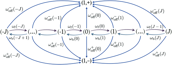
The dynamics of the two-motor runs can be investigated by considering the stochastic process on the discrete state space corresponding to the “stretching” or “compression” of the effective spring between the motors. In state (0) the spring is relaxed. If one of the motors performs a single step, the elastic spring of the two-motor system can be stretched or compressed by ![[small script l]](https://www.rsc.org/images/entities/char_e146.gif) /2 and the system undergoes a transition to states (1) or (−1), respectively, see the network representation in Fig. 4. In general, the motor system undergoes a forward transition from state (j) to state (j + 1) if kinesin or dynein performs a forward step. The corresponding stepping rates are given by α±(
/2 and the system undergoes a transition to states (1) or (−1), respectively, see the network representation in Fig. 4. In general, the motor system undergoes a forward transition from state (j) to state (j + 1) if kinesin or dynein performs a forward step. The corresponding stepping rates are given by α±(![[F with combining macron]](https://www.rsc.org/images/entities/i_char_0046_0304.gif) j>) for the individual motors which implies the forward rate
j>) for the individual motors which implies the forward rate| | ωf(j) = α+(![[F with combining macron]](https://www.rsc.org/images/entities/i_char_0046_0304.gif) j>) + α−( j>) + α−(![[F with combining macron]](https://www.rsc.org/images/entities/i_char_0046_0304.gif) j>) for (j) → (j + 1) j>) for (j) → (j + 1) | (2.22) |
with −J ≤ j ≤ J and the boundary condition ωf(J) = 0, see Fig. 4. Each forward transition leads to an increased stretching or a reduced compression of the elastic coupling between the two motors.
 |
| | Fig. 4 State space associated with different states of the elastic linker. The two states (1, +) and (1, −) are the absorbing states with a single plus and minus motor bound to the microtubule. States labelled by integer j with −J ≤ j ≤ J denote the states with a stretched and compressed linker for j > 0 and j < 0, respectively. Starting from state (j), the plus and minus motors unbind from the filament with rates ω+off(j) and ω−off(j). Furthermore, the motors undergo a forward transition from (j) to (j + 1) with rate ωf(j) and a backward transition from (j) to (j − 1) with rate ωb(j). | |
Likewise, the motor system undergoes a backward transition from state (j) to state (j − 1) if kinesin or dynein performs a backward step. The corresponding stepping rates are given by β±(![[F with combining macron]](https://www.rsc.org/images/entities/i_char_0046_0304.gif) j>) for the individual motors which implies the backward rate
j>) for the individual motors which implies the backward rate
| | ωb(j) = β+(![[F with combining macron]](https://www.rsc.org/images/entities/i_char_0046_0304.gif) j<) + β−( j<) + β−(![[F with combining macron]](https://www.rsc.org/images/entities/i_char_0046_0304.gif) j<) for (j) → (j − 1) j<) for (j) → (j − 1) | (2.23) |
with −
J ≤
j ≤
J and the boundary condition
ωb(−
J) = 0, see
Fig. 4. Each backward transition leads to a reduced stretching or an increased compression of the elastic coupling between the two motors.
In state (j), each of the motors can unbind (or detach) from the filament. The corresponding unbinding rates have the form
| | | ε±(Fj) = ε±0exp(|Fj|/F±d) ≡ ω±off(j) | (2.24) |
for the two types of motors. The overall unbinding rate from state (
j) is then given by
| | | ωoff(j) = ω+off(j) + ω−off(j). | (2.25) |
Motor parameters.
In the following, we will study the tug-of-war between one plus-directed motor and one minus-directed motor. Most single motor parameters will be kept fixed and assume values as appropriate for kinesin-1 and strong dynein, see Table 1. One parameter that we will vary systematically is the zero-force unbinding rateAs we will see, the elastically coupled tug-of-war is characterized, in the limit of small ε0, by essentially the same force balance as the MKL tug-of-war. Another parameter of the motor system that will be varied systematically is the elastic coupling between the two motors as described by the strain force FK = K![[small script l]](https://www.rsc.org/images/entities/char_e146.gif) = κ
= κ![[small script l]](https://www.rsc.org/images/entities/char_e146.gif) /2. In order to ensure that the finite size of the state space does not affect our results, we will always use a sufficiently large state space with (2J + 1) ≥ 101.
/2. In order to ensure that the finite size of the state space does not affect our results, we will always use a sufficiently large state space with (2J + 1) ≥ 101.
3 Results
3.1 Steady state properties of tug-of-war
The elastic coupling between the two antagonistic motors is only effective as long as both motors are attached to the filament and perform a 2-motor run. The latter runs are described by transitions between the states (j) in Fig. 4 and are terminated as soon as one of the motors unbinds from the filament. After such an unbinding event, the cargo is bound to the filament by a single motor as described by the states (1, +) and (1, −) in Fig. 4. These 1-motor runs continue until the unbound motor rebinds to the filament. We will assume that the rebinding typically leads to the state (0) which is relaxed in the sense that the two motors do not experience elastic interaction forces. Thus, after rebinding, a new 2-motor run starts from the initial state (0).
As described previously for the 2-motor runs of two identical motors,11,12 the steady state probability distribution as obtained from an ensemble average over many 2-motor runs can be replaced by a time average over a concatenated 2-motor run that is obtained by redirecting all transitions to the absorbing states towards a certain initial state. For the network depicted in Fig. 4, the absorbing states are provided by (1, +) and (1, −) and the initial state is taken to be the relaxed state (0). As a result, we obtain the redefined network in Fig. 12 which has no absorbing states. The corresponding steady state probability distribution can then be calculated by solving the master equation for the redefined network, see Appendix B.
The steady state probability distribution pstj describes the frequencies with which the effective elastic spring between the two motors has the extension j. The latter extension determines the spatial separation
| | L ≡ L0 + j![[small script l]](https://www.rsc.org/images/entities/char_e146.gif) | (3.1) |
of the two motors along the filament. The average motor–motor separation is then given by
| |  | (3.2) |
The fluctuating motor–motor separation
L should be directly accessible to experimental studies when one combines the recently introduced crosslinking of one fluo-labeled kinesin and one fluo-labeled dynein
via DNA hybridization
21 with advanced methods of fluorescence imaging such as FIONA.
29
In Fig. 5(a) we plot pstj for different values of the zero-force unbinding rate ε0. We see that for low unbinding rates, e.g. ε0 = 0.01 s−1, the probability distribution pstj shifts towards states with larger j-values. Because the elastic force Fj corresponding to spring extension j is given by Fj = jFK, we can transform the occupation probabilities of the states into the corresponding force distribution by a change of variables from j to Fj, see Fig. 5(b). As shown in the latter figure, a decrease in the unbinding rate leads to a shift of the force distribution towards higher force values and to an average elastic force
| |  | (3.3) |
that approaches the cargo force
Fca = 7 pN as obtained for velocity-matching. For higher unbinding rates, the occupation probabilities are shifted towards lower
j-values, leading to a reduced motor–motor separation and indicating that the motors are likely to unbind from the filament before reaching a state with velocity matching. The relationship in
(3.3) implies that the average elastic force 〈
F〉 can be determined from the average motor–motor separation 〈
L〉.
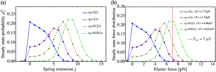 |
| | Fig. 5 (a) Steady state probability distributions pstj for different values of the unbinding rate ε0 as given in the inset. The spring extension j determines the spatial separation of the two motors via L0 + j![[small script l]](https://www.rsc.org/images/entities/char_e146.gif) . Apart from ε0, all parameters have the values as given in Table 1 for kinesin and strong dynein, which implies the strain force FK = 0.8 pN; and (b) steady state distributions for the elastic forces as obtained from pstj by a change of variables from j to Fj = jFK. The dashed vertical line (red) represents the cargo force Fca of the velocity-matched model. For low unbinding rates ε0, the average elastic force approaches this cargo force. For larger values of ε0, the force distribution becomes broader and shifts towards lower force values. As a consequence, the average elastic force 〈F〉 becomes smaller than the cargo force Fca, see average force values in the inset. Likewise, the average spatial separation L0 + 〈j〉 . Apart from ε0, all parameters have the values as given in Table 1 for kinesin and strong dynein, which implies the strain force FK = 0.8 pN; and (b) steady state distributions for the elastic forces as obtained from pstj by a change of variables from j to Fj = jFK. The dashed vertical line (red) represents the cargo force Fca of the velocity-matched model. For low unbinding rates ε0, the average elastic force approaches this cargo force. For larger values of ε0, the force distribution becomes broader and shifts towards lower force values. As a consequence, the average elastic force 〈F〉 becomes smaller than the cargo force Fca, see average force values in the inset. Likewise, the average spatial separation L0 + 〈j〉![[small script l]](https://www.rsc.org/images/entities/char_e146.gif) of the two motors decreases with increasing unbinding rate ε0 as follows from the distributions pstj in (a). of the two motors decreases with increasing unbinding rate ε0 as follows from the distributions pstj in (a). | |
3.2 Dependence of average elastic force on the unbinding rate
For two antagonistic motors coupled by an effective spring as studied here, the elastic interaction forces fluctuate and lead to steady state force distributions as shown in Fig. 5(b) for different values of the unbinding rate ε0. In contrast, for the MKL model, the mutual interaction force is given by the constant cargo force Fca as obtained via velocity matching, see Fig. 2. Inspection of Fig. 5(b) shows that the cargo force Fca provides a better approximation to the average elastic force 〈F〉 if the unbinding rate becomes smaller. To further examine the relationship between the fluctuating elastic forces and the cargo force, we now consider the very low unbinding rate ε0 = 10−5 s−1 and calculate the corresponding steady state probability distribution pstj. This distribution and the associated force distribution are displayed in Fig. 6 for different values of the strain force FK. Both for kinesin vs. strong dynein as depicted in Fig. 6(a1 and a2), and for kinesin vs. weak dynein in Fig. 6(b1 and b2), the cargo force Fca provides a more accurate approximation to the average elastic force 〈F〉 for smaller values of the strain force FK. This behaviour arises because smaller FK-values imply smaller changes in the elastic force induced by single motor steps which lead to a larger number of accessible force values and, thus, to a smoother interpolation of the discrete force distributions. In addition, the smaller cargo force for the tug-of-war between kinesin and weak dynein compared to kinesin and strong dynein implies that the force value F0 = 0 has a higher probability for the weak dynein case, see Fig. 6.
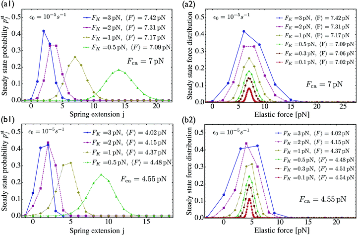 |
| | Fig. 6 Steady state probability distributions and force distributions for the small unbinding rate ε0 = 10−5 s−1 and for different choices of the strain force FK: (a1 and a2) kinesin against strong dynein, see the motor parameters in Table 1. As we decrease FK, the average force 〈F〉 approaches the cargo force Fca = 7 pN more accurately; and (b1 and b2) kinesin against weak dynein, see again Table 1. The cargo force now has the lower value Fca = 4.55 pN compared to the kinesin vs. strong dynein case in (a). Accordingly, the state (0) in (b1) has a higher occupation probability than the same state in (a1), and the probability for the force value F0 = 0 is increased in (b2) compared to (a2). | |
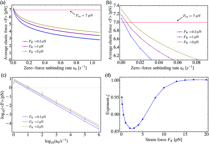
As shown in Fig. 5, increasing the unbinding rate ε0 leads to a reduction in the average elastic force 〈F〉 induced by the motors. This unbinding rate dependence of the average elastic force is displayed in more detail in Fig. 7(a) for different choices of the strain force FK, with Fig. 7(b) magnifying the limit of small ε0. In this limit, the deviation of the average elastic force 〈F〉 from the cargo force Fca increases for larger values of FK. The decrease of the average force 〈F〉 with increasing unbinding rate ε0 is caused by the increasing probability that one of the motors unbinds from the filament before the motors have matched their velocities in the 2-motor run and, thus, before the motors can generate forces comparable to the cargo force Fca. The double-logarithmic plot in Fig. 7(c) reveals that the average elastic force 〈F〉 decays to zero for large ε0. It follows from eqn (3.3) that the asymptotic behavior of 〈F〉 for large ε0 is determined by the asymptotic behavior of the steady state probability distribution pstj for large ε0. The latter behavior can be directly obtained from the master equations (B.1)–(B.4). One then finds from the local flux balance in the states (j) that
| |  | (3.4) |
and
| |  | (3.5) |
in the limit of large unbinding rates
ωoff(
j) ∼
ε0. Iterating these relations and imposing the normalization condition
(B.5), one obtains the asymptotic behavior
| |  | (3.6) |
as well as
| | pst0 ≈ 1 − pst1 − pst−1 = 1 + ![[scr O, script letter O]](https://www.rsc.org/images/entities/char_e52e.gif) (1/ε0) for large ε0 (1/ε0) for large ε0 | (3.7) |
whereas all other
pstj are of higher order in 1/
ε0. The average elastic force 〈
F〉 as given by (3.3) then behaves as
| | | 〈F〉 ≈ FK(pst1 − pst−1) ∼ 1/ε0 for large ε0. | (3.8) |
The power law behavior 〈
F〉 ∼ 1/
ε0 is corroborated by the numerical data in
Fig. 7(c) which are well fitted, over the accessible range of
ε0-values as given by 1 s
−1 ≤
ε0 ≤ 10
6 s
−1, by a power-law of the form 〈
F〉 ∼ 1/
εζ with the effective decay exponent
ζ. As shown in
Fig. 7(d), the effective exponent
ζ is found to depend weakly on the strain force
FK for
FK < 13 pN and to approach the true asymptotic value
ζ = 1 for
FK > 13 pN.
 |
| | Fig. 7 (a) Average elastic force 〈F〉 acting on the motors as a function of the zero-force unbinding rate ε0 for different values of the strain force FK. The average force 〈F〉 decreases with increasing ε0, irrespective of the value for FK; (b) limiting behaviour of the average elastic force 〈F〉 for small unbinding rate ε0. In this limit, the average force 〈F〉 approaches an asymptotic value 〈F〉0 close to the cargo force Fca and the deviation 〈F〉0 − Fca decreases with decreasing FK; (c) double-logarithmic plot of the average force 〈F〉 versus the unbinding rate which now varies over six orders of magnitude. The straight lines clearly demonstrate that 〈F〉 decays to zero for large ε0 and that this decay can be well fitted, over the accessible range of ε0-values, by a power law of the form 〈F〉 ∼ 1/εζ0 with the effective decay exponent ζ; and (d) effective exponent ζ as obtained by fitting the data in (c) for different values of the strain force FK. | |
3.3 Statistics of elastic forces for vanishing unbinding rate
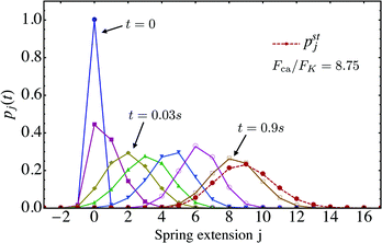
We now look at the properties of the tug-of-war in the limit in which the two motors can no longer unbind from the filament, corresponding to zero-force unbinding rate ε0 = 0 which implies that ωoff(j) = 0 for all j. In this case, the state space for the tug-of-war between the two motors is reduced to the states j = −J,…,+J. For this reduced state space, the probability distribution pj(t), which starts from the initial distribution pj(0) = δj0 at time t = 0, evolves towards a steady state distribution pstj as shown in Fig. 8. The maximum of pstj is located close to the state (j = 9) characterized by the elastic force 9FK = 7.2 pN induced by the effective spring, while the cargo force obtained from velocity matching is Fca = 7 pN.
 |
| | Fig. 8 Time evolution of the probability distribution pj(t) for unbinding rate ε0 = 0 and strain force FK = 0.8 pN, the latter parameter being appropriate for strong dynein. The initial probability distribution at time t = 0 is given by pj(0) = δj0 corresponding to a relaxed spring with zero extension. As t increases, the distribution pj(t) approaches the steady state distribution pstj as indicated by the dashed red line. | |
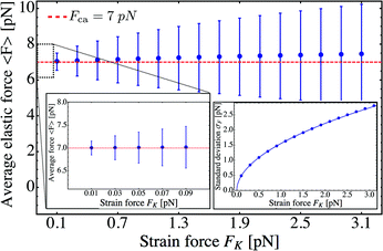
The average elastic force 〈F〉 for the process with vanishing unbinding rate is shown in Fig. 9 for different values of the strain force FK. We observe that, regardless of the choice of FK, the average force 〈F〉 remains close to the cargo force Fca whereas its standard deviation σF increases with increasing FK. In the limit of small strain forces FK, the average force 〈F〉 approaches the cargo force Fca more accurately, in accordance with our previous results. As shown in the right inset of Fig. 9, the standard deviation
| |  | (3.9) |
of the elastic force behaves as
| |  | (3.10) |
over the whole range of
FK-values considered here. For
FK = 1 pN and
ε0 = 0, the standard deviation is
σF ≃ 1.5 pN. Increasing the zero-force unbinding rate
ε0 for fixed
FK = 1 pN, the full network in
Fig. 4 leads to a slight increase in the deviation
σF, which then saturates at
σF ≃ 1.9 pN for an unbinding rate of
ε0 = 1 s
−1 (data not shown here).
 |
| | Fig. 9 Average elastic force 〈F〉 as a function of strain force FK for unbinding rate ε0 = 0: the average force 〈F〉 is roughly independent of FK for FK < 3 pN and remains close to the cargo force value Fca = 7 pN. (left inset) Average force 〈F〉 for 0.01 pN ≤ FK ≤ 0.09 pN. (right inset) The standard deviation σF of the elastic force is proportional to  (solid blue line). (solid blue line). | |
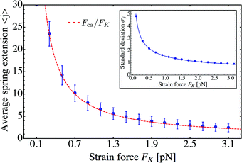
Using these results for the statistics of the elastic forces, we can directly conclude that the average spring extension 〈j〉 behaves as
| | | 〈j〉 = 〈F〉/FK ≃ Fca/FK | (3.11) |
and its standard deviation
| |  | (3.12) |
as
| |  | (3.13) |
These dependencies on the strain force
FK are displayed in
Fig. 10.
 |
| | Fig. 10 Average spring extension 〈j〉 and standard deviation σj of these extensions as a function of strain force FK for unbinding rate ε0 = 0. Both 〈j〉 and σj decrease with increasing FK. The FK-dependence of 〈j〉 is very well described by Fca/FK (dashed red line). The standard deviation σj is proportional to  (full blue line in the inset). This behavior is intimately related to the behavior of the average force 〈F〉 and the associated standard deviation σF, see the main text. (full blue line in the inset). This behavior is intimately related to the behavior of the average force 〈F〉 and the associated standard deviation σF, see the main text. | |
The average spring extension 〈j〉 implies that the two motors have the average separation 〈ΔL〉 = ![[small script l]](https://www.rsc.org/images/entities/char_e146.gif) 〈j〉. Thus, we conclude that, in the limit of small FK corresponding to weakly coupled motors, the average separation between the motors increases as
〈j〉. Thus, we conclude that, in the limit of small FK corresponding to weakly coupled motors, the average separation between the motors increases as  . Furthermore, the behavior of the standard deviation σj is consistent with a Gaussian probability distribution of the form
| | | pstj ∝ exp[−cK(j − 〈j〉)2] | (3.14) |
for the spring extension
j where
c is a proportionality factor.
It is instructive to compare the distribution as given by (3.14), which arises from the stochastic nature of the tug-of-war and the underlying motor activity, with the equilibrium distribution
| | | peqj ∝ exp[−½Kj2/(kBT)] | (3.15) |
corresponding to thermal fluctuations in the harmonic spring potential ½
Kj2. Comparing the two distributions in
(3.14) and (3.15), we can draw two conclusions. First, the motor activity leads to a nonzero average value 〈
j〉 of the spring extension implying a nonzero average separation 〈Δ
L〉 =
![[small script l]](https://www.rsc.org/images/entities/char_e146.gif)
〈
j〉 of the motors and a nonzero average force 〈
F〉 =
FK〈
j〉 acting on them. Second, the fluctuations around the average value 〈
j〉 can be characterized by a standard deviation

both for the thermal and for the active process.
A comparison between Fig. 7 and 9 also shows that the tug-of-war obtained for the reduced state space with ε0 = 0 is reached in a smooth manner when we consider the full state space as depicted in Fig. 4 and take the limit of small ε0. This agreement is to be expected because the steady state probability distributions for ε0 > 0 follow from the redefined network in Fig. 12 which also becomes identical with the reduced state space for ε0 = 0.
3.4 Relaxation time for vanishing unbinding rate
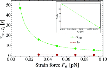
For the reduced state space consisting of the states (j) with j = −J,…,+J as obtained for unbinding rate ε0 = 0, the elastically coupled motors eventually reach a steady state with the average elastic force 〈F〉 ≃ Fca as illustrated in Fig. 8 for FK = Fca/8.75. We will now address the relaxation time for this process, i.e. the time it takes to actually reach this steady state. This relaxation time τre is provided by the largest non-zero eigenvalue λ2 of the transition rate matrix for the redefined state space in Fig. 12via the relation30
As shown in Fig. 11, the relaxation time τre for the approach towards the steady state increases strongly as we reduce the strain force FK, i.e. as we reduce the elastic coupling between the two motors and allow them to move further apart. Indeed, in the limit of small FK, the average separation of the two motors increases as 〈ΔL〉 = ![[small script l]](https://www.rsc.org/images/entities/char_e146.gif) 〈j〉 ∼ 1/FK as follows from the behavior of 〈j〉 in Fig. 10. When we plot the τre-data in a double-logarithmic manner, see the inset of Fig. 11, a least-squares fit leads to the relation τre ∼ 1/FηK with the decay exponent η = 0.97. We thus conclude that the relaxation time τre is also inversely proportional to FK to a very good approximation. As a consequence, the relaxation time τre for two weakly coupled motors is roughly proportional to their average separation 〈ΔL〉 ∼ 1/FK which diverges in the limit of small FK =
〈j〉 ∼ 1/FK as follows from the behavior of 〈j〉 in Fig. 10. When we plot the τre-data in a double-logarithmic manner, see the inset of Fig. 11, a least-squares fit leads to the relation τre ∼ 1/FηK with the decay exponent η = 0.97. We thus conclude that the relaxation time τre is also inversely proportional to FK to a very good approximation. As a consequence, the relaxation time τre for two weakly coupled motors is roughly proportional to their average separation 〈ΔL〉 ∼ 1/FK which diverges in the limit of small FK = ![[small script l]](https://www.rsc.org/images/entities/char_e146.gif) K =
K = ![[small script l]](https://www.rsc.org/images/entities/char_e146.gif) κ/2.
κ/2.
 |
| | Fig. 11 Strain force dependence of the relaxation time τre (green) needed to attain the steady state for unbinding rate ε0 = 0. The inset displays a double-logarithmic plot of the τre-data. A least-squares fit to these data leads to τR ∼ 1/FηK with the exponent η = 0.97 from which we conclude that the relaxation time τre is inversely proportional to FK to a very good approximation. For comparison, the average run time t2 (red) for 2-motor runs with ε0 = 0.3 s−1 has also been included. For the range of FK-values considered here, the relaxation time τre is always large compared to the average run time t2. | |
In order to obtain a well-defined relaxation time τre, we had to consider the limiting case with unbinding rate ε0 = 0. Real motors have, of course, a finite unbinding rate which implies that their 2-motor runs are terminated after a finite time and can then be characterized by the average run time  . We must now distinguish different cases depending on the relative size of the average run time t2 and the relaxation time τre. If t2 is large compared to τre, the two motors will be characterized by an average elastic force 〈F〉 close to the cargo force Fca of the MKL model. On the other hand, if t2 is small compared to τre, the force balance between the two motors is different because 〈F〉 is small compared to Fca. As shown in Fig. 11, the latter case applies to the unbinding rate ε0 = 0.3 s−1 for the whole range of FK-values considered in this figure. A more detailed discussion of the different timescales and the associated dynamic regimes will be given in a subsequent publication.31
4 Summary and outlook
In this paper, we considered the tug-of-war between one kinesin and one dynein motor, which are coupled to a common cargo via elastic linkers. We started from the known properties of the single motors and used these properties to derive the force-dependent stepping rates for forward and backward steps of both motors. Unexpectedly, we found that the backward stepping rate of strong dynein exhibits a maximum at an intermediate load force, see Fig. 1. We then described the elastic interaction forces between the motors and the cargo by two harmonic springs which can be combined into an effective harmonic spring between the two motors. The extension j of this effective spring was used to define the state space for the tug-of-war between two elastically coupled motors as displayed in Fig. 4.
A Markov process was constructed on this state space with transition rates that were derived from the single motor rates. Starting from the relaxed state (0) with spring extension j = 0, the antagonistic motors perform a 2-motor run on the reduced state space consisting of the transient states (j) with j = −J,…,+J until one motor unbinds from the filament and the process ends up in one of the absorbing states (1, +) or (1, −), see Fig. 4. The ensemble average over many such 2-motor runs can be obtained by computing the steady state probability distribution pstj on the redefined state space in Fig. 12. Using this distribution, we calculated the average elastic force 〈F〉 experienced by the two motors as a function of the unbinding rate ε0, see Fig. 7. This average force approaches the cargo force Fca for small ε0 and decays to zero as 1/ε0 for large ε0, see (3.8). Numerically we find the power law 〈F〉 ∼ 1/εζ0 with an effective decay exponent ζ that depends on the strain force FK, see Fig. 7(d).
 |
| | Fig. 12 Redefined state space: all transitions of the full network in Fig. 4 that reach the two absorbing states (1, +) and (1, −) are combined with a very fast rebinding transition towards the transient initial state (0). Because the rebinding process is instantaneous, the combined unbinding and rebinding transition from state (j) to state (0) is governed by the rate ωoff as given by eqn (2.25). | |
Finally, we studied the limiting case of a tug-of-war between two elastically coupled motors that cannot unbind from the filament, corresponding to zero-force unbinding rate ε0 = 0. In this case, we found that the time evolution of the probability distribution always leads to a steady state distribution for which (i) the average elastic force 〈F〉 is close to the cargo force Fca irrespective of the strain force FK and (ii) the standard deviation σF of the force fluctuations is proportional to  as shown in Fig. 9. These relationships imply that the average spring extension 〈j〉 ∼ 1/FK ∼ 1/K and the standard deviation
  , see Fig. 10. The latter dependence is consistent with a Gaussian probability distribution for the spring extension j as described by (3.14). The behavior of the average spring extension 〈j〉 implies that the average separation 〈ΔL〉 =
 ![[small script l]](https://www.rsc.org/images/entities/char_e146.gif) 〈j〉 of the two antagonistic motors increases as 1/K for small K, corresponding to the weak coupling limit. Essentially the same K-dependence is found for the relaxation time τre towards the steady state probability distribution pstj, see Fig. 11. Therefore, in the weak coupling limit of small K, both the average motor separation 〈ΔL〉 and the relaxation time τre diverge as 1/K for ε0 = 0.
〈j〉 of the two antagonistic motors increases as 1/K for small K, corresponding to the weak coupling limit. Essentially the same K-dependence is found for the relaxation time τre towards the steady state probability distribution pstj, see Fig. 11. Therefore, in the weak coupling limit of small K, both the average motor separation 〈ΔL〉 and the relaxation time τre diverge as 1/K for ε0 = 0.
In the present article, we have focussed on the forces acting between two elastically coupled motors. As indicated in the last subsection 3.4 on the relaxation time, the resulting tug-of-war involves different timescales that define different kinetic regimes. Likewise, as far as motor unbinding is concerned, one has to distinguish spontaneous unbinding for small elastic forces from force-induced unbinding for large elastic forces. Another interesting topic is the tug-of-war between elastically coupled motor teams involving N1 ≥ 1 plus-directed motors and N2 ≥ 1 minus-directed motors. These more complex motor systems will be addressed in a forthcoming paper.31
As previously mentioned, the theoretical results presented here can be scrutinized by experimental in vitro studies based on recently developed protocols16–20 to control the number of active motors on synthetic DNA scaffolds. Evidence for a tug-of-war mechanism between kinesin and dynein attached to such scaffolds was observed in ref. 19 and 20. Very recently, it has also been demonstrated that one can directly crosslink a single, fluo-labeled kinesin with a single, fluo-labeled dynein via DNA hybridization.21 Our tug-of-war model provides detailed predictions for the transport properties of such a two-motor system. One of these properties is the probability distribution pstj for the spatial separation of the two motors as displayed in Fig. 5a, 6a1, b1, and 8. The latter distribution should be accessible to advanced methods of fluorescence imaging such as FIONA.29 In principle, it is also possible to measure the average interaction force 〈F〉 directly via FRET-based molecular tension probes32 that are incorporated into the linkers between the motors and the cargo. Other quantities of interest that can be used to compare our theory with experiment include the run lengths and run times of the two-motor systems.
Appendices
A Review of tug-of-war with velocity matching
Here we shortly describe the tug-of-war in the MKL model, following ref. 6 and 7. Let N+ and N− denote the number of plus and minus motors attached to the cargo, respectively. At any given time t′ the cargo is pulled by n+ plus and n− minus motors, where 0 ≤ n+ ≤ N+ and 0 ≤ n− ≤ N−. The motility state of the cargo at t′ is then characterised by the number of bound motors to the microtubule, denoted by (n+, n−). Assuming that (i) opposing motors act as load and (ii) identical motors share this load6 the transition rates between adjacent motility states can be inferred from single motor binding and unbinding behaviour. The force balance on a cargo pulled by n+ plus and n− minus motors at any moment is given by:| | | Fca(n+,n−) ≡ n+F+ = −n−F−. | (A.1) |
F+ and F− are the forces “felt” by a single plus and a single minus motor, respectively. The sign of the force is chosen to be positive if it is a load on the plus motors. The force acting on a single plus motor is then given by F+ = Fca(n+,n−)/n+. This means that all plus motors feel the same load in a given cargo state (n+,n−). The effective unbinding rate for a plus motor is:| | ε+(n+,n−) = n+ε+0![[thin space (1/6-em)]](https://www.rsc.org/images/entities/char_2009.gif) exp(|Fca(n+,n−)|/(n+F+d)). exp(|Fca(n+,n−)|/(n+F+d)). | (A.2) |
Note that multiplying single motor rates by the factor n+ implies that the motor–motor interactions are not considered. The effective binding rate of a plus motor is similarly given by:| | | π+(n+,n−) = (N+ − n+)π+0. | (A.3) |
The effective binding and unbinding rates for the minus motors can be obtained by replacing the index “+” by “−” in eqn (A.2) and (A.3).
An expression for the cargo force Fca(n+,n−) of the force balance condition can be determined by observing that both plus and minus motor teams match their velocities under this load. The corresponding velocity is equal to the cargo velocity:
| | | vca(n+,n−) = v+(Fca(n+,n−)/n+) = −v−(Fca(n+,n−)/n−), | (A.4) |
where the functions
v+(·) and
v−(·) are determined by the single plus and minus motor force–velocity relations. In
ref. 6 and 7 the force–velocity relation of a single motor is given by the following piecewise-linear function:
| | | v(F) = vF|B(1 − F/Fs), | (A.5) |
with
vF|B =
vF for
F ≤
Fs and
vF|B =
vB for
F >
Fs, where
vF and
vB are the force-free forward and backward velocity, respectively. When there is no load force acting on the motor, it proceeds with the force-free forward velocity
vF. Note that both
vF and
vB indicate the absolute values of the corresponding velocities. In this work, however, we use an empirical force–velocity relation obtained by a least squares fit to the data from
ref. 22. This specific choice is initially presented in
ref. 11, see
eqn (2.1) in the main text.
From eqn (A.5) we obtain the velocity of plus motors for the state (n+,n−):
| |  | (A.6) |
The minus motor velocity is given by an analogous expression by replacing the index “+” by “−”. The cargo force
Fca(
n+,
n−) can now be determined by the velocity matching condition in
eqn (A.4):
| |  | (A.7) |
Observe that when only one motor type is active,
i.e. n− = 0 or
n+ = 0, the force acting on the cargo disappears:
Fca(
n+,
n−) = 0. From
eqn (A.7) and (A.4), we obtain the cargo velocity:
| |  | (A.8) |
For the empirical force–velocity relationship v(F) as given in the main text by eqn (2.1) the matching condition (A.4) can be solved numerically. In the case of two antagonistic motors the cargo velocity defined by the matching condition eqn (A.4) can be obtained graphically from the intersection point (F,v) = (Fca,vca) of two force–velocity relations, as shown in Fig. 2.
For the case of “stronger plus motors”, i.e. n+F+s > n−F−s, we have:
| | | Fca(n+,n−) = Λn+F+s + (1 − Λ)n−F−s, | (A.9) |
| |  | (A.10) |
where
Λ = (1 + (
n+F+sv−B)/(
n−F−sv+F))
−1. Observe that
Λ can only have values in the interval [0,1], which implies that the cargo force
Fca(
n+,
n−) ranges between the maximal values of the plus and minus stall forces
n+Fs+ and
n−Fs−.
In this work we only consider two opposing motors, i.e. the state (n+ = 1, n− = 1). The notation used in the main text is Fca ≡ Fca(n+ = 1, n− = 1) and vca ≡ vca(n+ = 1, n− = 1), where Fca and vca are obtained from the numerical solution of the velocity matching condition, i.e. by determining the coordinates of the intersection point of the force–velocity functions of both motors.
B Master equations and the specification of parameters
The full network in Fig. 4 can be reduced to a closed network with all transitions to the two absorbing states being redirected to the initial state (0), see Fig. 12. The steady state distribution of the closed network can now be used to obtain some quantities of interest such as the average absorption time for the full network.11,33 The latter quantity can also be calculated recursively without constructing the closed network.34 A single trajectory on the closed network in Fig. 12 corresponds to the concatenation of many full network trajectories, each of which starts at the initial state (0) and is eventually absorbed in the states (1, +) or (1, −). The master equations corresponding to the closed network in Fig. 12 are given by| | | ∂tp−J(t) = −[ωf(−J) + ωoff(−J)]p−J(t) + ωb(−J + 1)p−J+1(t) | (B.1) |
and| | | ∂tpJ(t) = −[ωb(J) + ωoff(J)]pJ(t) + ωf(J − 1)pJ−1(t). | (B.2) |
for the two boundary states with j = −J and j = +J, by| |  | (B.3) |
for the state (0), where the sum includes all states (j) apart from (0), and| | | ∂tpj(t) = −[ωf(j) + ωb(j) + ωoff(j)]pj(t) + ωb(j + 1)pj+1(t) + ωf(j − 1)pj−1(t) | (B.4) |
for all other values of j. Eqn (B.1)–(B.4) are supplemented by the normalization condition| |  | (B.5) |
The different rates that appear in these equations are defined in (2.22)–(2.25) and depend on the single motor properties described by (2.1)–(2.6). The latter relationships involve the single motor parameters v0, vmax, vmin, Fs, q0, Fd, ε0, and ![[small script l]](https://www.rsc.org/images/entities/char_e146.gif) as well as the elastic coupling parameter K = κ/2. We typically vary one parameter such as the unbinding rate ε0 or the elastic coupling parameter K, keeping all other parameters fixed at their values in Table 1.
as well as the elastic coupling parameter K = κ/2. We typically vary one parameter such as the unbinding rate ε0 or the elastic coupling parameter K, keeping all other parameters fixed at their values in Table 1.
C Matrix form of master equations
The master equations can be written in the matrix form if we define the (2J + 1)-dimensional column vector| | | (p−J(t),p−J+1(t),…,pJ−1(t),pJ(t))T ≡ |p(t)〉 | (C.1) |
where the superscript T stands for ‘transpose’ and the ket notation will be used for convenience. Using the latter vector, the master equations (B.1)–(B.4) attain the compact formwith the (2J + 1) × (2J + 1) transition rate matrix W. The diagonal matrix elements Wj,j are given by| | | Wj,j = −[ωf(j) + ωb(j) + ωoff(j)] for j ≠ −J, j ≠ 0, and j ≠ J | (C.3) |
as well as by| | | W−J,−J = −[ωf(−J) + ωoff(−J)], | (C.4) |
| | | W0,0 = −[ωf(0) + ωb(0)], | (C.5) |
and| | | WJ,J = −[ωb(J) + ωoff(J)]. | (C.6) |
The off-diagonal matrix elements of W are given by| | | Wj,j+1 = ωb(j + 1) for j ≤ J − 1 | (C.7) |
and| | | Wj,j−1 = ωf(j − 1) for j ≥ −J + 1. | (C.8) |
For each column of the matrix W, the matrix elements sum up to zero, i.e. for all values of k.
Most of our results are based on the steady state solutions pstj of eqn (C.2) with ∂t|pst〉 = W|pst〉 = 0 or
| |  | (C.9) |
The numerical solutions of these equations were obtained with a self-written script based on built-in subroutines of
Mathematica 9.0.
D Time evolution without motor unbinding
In Section 3.3, we describe the time evolution of the probability distribution pj(t) for unbinding rate ε0 = 0, see Fig. 8. In this limiting case, the state space in Fig. 4 becomes 1-dimensional and does not contain any cycles. The steady state probability distribution pstj then satisfies the detailed balance conditions| | | ωf(j − 1)pstj−1 − ωb(j)pstj = Wj,j−1pstj−1 − Wj−1,jpstj = 0 | (D.1) |
for all j with −J ≤ j ≤ J − 1 which is equivalent tofor all nonzero matrix elements. Applying the conditions (D.1) iteratively along the 1-dimensional state space, we obtain the steady state solutions| |  | (D.3) |
where pst−J is determined by the normalization condition  .
.
In general, the matrix W is not symmetric. However, if the matrix elements Wi,j fulfill the detailed balance conditions (D.2), we can define the symmetric transition rate matrix ![[W with combining tilde]](https://www.rsc.org/images/entities/b_char_0057_0303.gif) with matrix elements41
with matrix elements41
| |  | (D.4) |
Because the matrix
![[W with combining tilde]](https://www.rsc.org/images/entities/b_char_0057_0303.gif)
is symmetric, it has real eigenvalues
λn with
n = 1,2,…,
N and
N = 2
J + 1. Furthermore, the right and left eigenvectors for the eigenvalue
λn have the same components
ũj(
λn),
i.e.| |  | (D.5) |
and satisfy the orthonormality condition
| |  | (D.6) |
where the Kronecker delta symbol
δm,n = 1 for
m =
n and 0 otherwise.
It then follows from eqn (D.4) that the transition rate matrix W has the same eigenvalues λn as the symmetric matrix ![[W with combining tilde]](https://www.rsc.org/images/entities/b_char_0057_0303.gif) and that the right eigenvectors of W are given by the column vectors
and that the right eigenvectors of W are given by the column vectors
| |  | (D.7) |
whereas the left eigenvectors of
W are provided by the row vector
| |  | (D.8) |
The left and right eigenvectors satisfy the orthonormality and completeness relations
| |  | (D.9) |
with the identity matrix
1. The column vector |
p(
t)〉 can now be decomposed according to
| |  | (D.10) |
When this decomposition is inserted into the master equation
(C.2), we obtain the time-dependent coefficients
Cn(
t) =
Cn(0)e
λnt and the probabilities
| |  | (D.11) |
with
| |  | (D.12) |
Because all eigenvalues
λn are negative for
n ≥ 2, the long time behavior of
pj(
t) is dominated by the term with
n = 1 and
λ1 = 0 corresponding to the steady state probabilities
pstj.
Thus, in order to determine the time-dependent probabilites pj(t) as given by (D.11), we subsequently computed the steady state probabilities pstj, see (D.3), the symmetric matrix ![[W with combining tilde]](https://www.rsc.org/images/entities/b_char_0057_0303.gif) via(D.4), as well as the eigenvalues λn of
via(D.4), as well as the eigenvalues λn of ![[W with combining tilde]](https://www.rsc.org/images/entities/b_char_0057_0303.gif) and the corresponding eigenvectors with components ũj(λn), using again the built-in subroutines of Mathematica 9.0. The initial distributions were set to pj(t = 0) = 1 for j = 0 and pj(t = 0) = 0 for all other values of j.
and the corresponding eigenvectors with components ũj(λn), using again the built-in subroutines of Mathematica 9.0. The initial distributions were set to pj(t = 0) = 1 for j = 0 and pj(t = 0) = 0 for all other values of j.
E Dependence of average elastic force on strain force
In Fig. 9 the strain force dependency of the average elastic force 〈F〉 is presented up to a strain force value of FK ≃ 3 pN. In this regime, the average elastic force is approximately independent of the strain force and equal to the cargo force Fca of the tug-of-war in the MKL model. In the limit of high strain forces, however, we would expect the elastically coupled model to generate 〈F〉 = 0, since none of the motors would be able to make a single step because of the high spring stiffness.
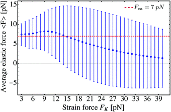
In Fig. 13 we plot the average force 〈F〉 as a function of the strain force FK within the range 3 pN ≤ FK ≤ 40 pN. We observe a weak maximum of 〈F〉 around a strain force value of FK ≃ 10 pN. For FK ≥ 15 pN, the average force 〈F〉 decreases monotonically towards zero. Considering the steady state distribution over the discrete state space one can interpret the FK-dependence of 〈F〉 as follows. Up to a strain force value of FK ≃ 2F+s = 2F−s the process can perform at least one step resulting in a stretching of the linker between the motors. Recall that the transition from state (0) to state (1) occurs with the sum of forward stepping rates α+(![[F with combining macron]](https://www.rsc.org/images/entities/i_char_0046_0304.gif) 0>) + α−(
0>) + α−(![[F with combining macron]](https://www.rsc.org/images/entities/i_char_0046_0304.gif) 0>), see eqn (2.22), where the motors feel the effective force
0>), see eqn (2.22), where the motors feel the effective force ![[F with combining macron]](https://www.rsc.org/images/entities/i_char_0046_0304.gif) 0> = FK/2. For a strain force of FK = 14 pN this force is
0> = FK/2. For a strain force of FK = 14 pN this force is ![[F with combining macron]](https://www.rsc.org/images/entities/i_char_0046_0304.gif) 0> = 7 pN = F+s = F−s, at which the motors are equally likely to perform a forward or a backward step. Without motor unbinding, and taking into account that a further transition from (1) to (2) with an effective force of
0> = 7 pN = F+s = F−s, at which the motors are equally likely to perform a forward or a backward step. Without motor unbinding, and taking into account that a further transition from (1) to (2) with an effective force of ![[F with combining macron]](https://www.rsc.org/images/entities/i_char_0046_0304.gif) 1> = 14 pN acting on the motors is highly unlikely, this force balance is expected to lead to steady state probabilities pst0 ≃ pst1 ≃ 0.5 and to the average elastic force 〈F〉 ≃ pst0F0 + pst1F1 = 7 pN = Fca.† A further increase in the strain force FK shifts the steady state distribution towards the relaxed state (0), i.e. pst0 > pst1, resulting in a reduction of the average force 〈F〉 towards zero. The initial increase of 〈F〉 with increasing FK implies that the corresponding increase in F1 overcompensates the decrease of pst1 for FK < 10 pN, see the steady state distribution in Fig. 14.
1> = 14 pN acting on the motors is highly unlikely, this force balance is expected to lead to steady state probabilities pst0 ≃ pst1 ≃ 0.5 and to the average elastic force 〈F〉 ≃ pst0F0 + pst1F1 = 7 pN = Fca.† A further increase in the strain force FK shifts the steady state distribution towards the relaxed state (0), i.e. pst0 > pst1, resulting in a reduction of the average force 〈F〉 towards zero. The initial increase of 〈F〉 with increasing FK implies that the corresponding increase in F1 overcompensates the decrease of pst1 for FK < 10 pN, see the steady state distribution in Fig. 14.
 |
| | Fig. 13 Average elastic force 〈F〉 of the process for zero-force unbinding rate ε0 = 0 and strain forces FK ≥ 3 pN. We observe that 〈F〉 reaches a maximum around a strain force value of FK = 10 pN. For larger strain forces corresponding to stiffer springs, the average force 〈F〉 induced by the motors decreases monotonically to zero. | |
 |
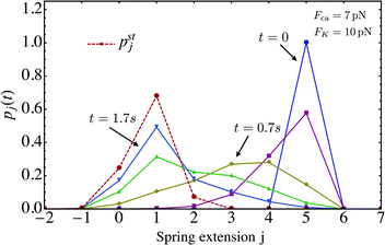
| | Fig. 14 Time evolution of the probability distribution pj(t) for a strain force of FK = 10 pN. The initial probability distribution is pj(0) = δj5. The probability distribution pj(t) approaches the steady state distribution pstj, indicated by the dashed red line, which has a maximum for spring extension j = 1. | |
In Fig. 14 we plot the time evolution of the probability distribution over the states pj(t) starting from an initial state different from (0). We fix a high strain force FK = 10 pN, corresponding to the maximum of 〈F〉 in Fig. 13, and choose the initial state to be (5), i.e. pj(0) = δj5. As t increases we see that the time-dependent probability distribution pj(t) approaches the steady state distribution pstj (dashed red line). We see that pstj has a clear peak in state (1), but also a nonzero value in (2), where the corresponding elastic force is given by F2 = 2FK = 20 pN. These high force value contributions from state (2) to the average force results in 〈F〉 > Fca, as observed in Fig. 13.
F Dependence of force distribution on the size of state space
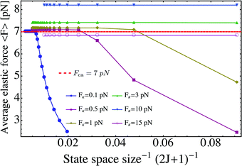
As shown in Fig. 10, the probability distribution pstj is shifted towards larger j-values and becomes broader as we decrease the strain force FK. Therefore, a fixed size of the state space, i.e. a fixed number (2J + 1) of states, acts to truncate the distribution pstj for sufficiently small values of FK. Likewise, the average elastic force 〈F〉 starts to decrease, for a fixed value of FK, as we decrease the size (2J + 1) of the state space below a certain minimal value.
These finite size effects are illustrated in Fig. 15 where the average elastic force 〈F〉 is plotted as a function of the inverse size (2J + 1)−1 of the state space. Inspection of this figure shows that 〈F〉 attains a constant value for sufficiently small (2J + 1)−1 but decays strongly for sufficiently large (2J + 1)−1. In practice, we chose (2J + 1) ≥ 201 for FK ≤ 0.1 pN and (2J + 1) ≥ 51 for FK ≤ 0.5 pN.
 |
| | Fig. 15 Dependence of average elastic force 〈F〉 on the inverse size (2J + 1)−1 of the state space. If the two motors are weakly coupled, the finite size of the state space acts to truncate the probability distributions. Thus, for FK = 0.1 pN, we see large finite size effects and a strong decay of 〈F〉 already for (2J + 1)−1 ≳ 0.005. | |
Glossary of mathematical symbols
|
α(F) | Force-dependent forward stepping rate |
|
β(F) | Force-dependent backward stepping rate |
|
δ
ij
| Kronecker delta symbol |
|
ε
0
| Zero-force unbinding rate |
|
ε(F) | Force-dependent unbinding rate |
|
ζ
| Effective decay exponent in 〈F〉 ∼ ε−ζ0, see Fig. 7 |
|
η
| Decay exponent in τre ∼ F−ηK, see Fig. 11 |
|
F
ca
| Cargo force of the MKL model |
|
F
d
| Detachment force |
|
F
s
| Stall force |
|
F
dy,ca
| Force exerted by the dynein motor onto the cargo |
|
F
ki,ca
| Force exerted by the kinesin motor onto the cargo |
|
F
j
| Elastic force acting in state (j), defined by Fj ≡ jFK |
![[F with combining macron]](https://www.rsc.org/images/entities/i_char_0046_0304.gif) j>
j>
| Effective force acting during the stretching by a single step |
![[F with combining macron]](https://www.rsc.org/images/entities/i_char_0046_0304.gif) j<
j<
| Effective force acting during the compression by a single step |
|
F
K
| Effective strain force, FK = K![[small script l]](https://www.rsc.org/images/entities/char_e146.gif) |
|
F
±
| Force acting on single plus/minus motors in the MKL model |
|
j
| Integer spring extension in units of ![[small script l]](https://www.rsc.org/images/entities/char_e146.gif) , −J ≤ j ≤ J , −J ≤ j ≤ J |
| (j) | State corresponding to the spring extension j |
|
J
| Maximal value of j |
|
κ
| Spring constant of a single motor linker |
|
K
| Effective spring constant, K = κ/2, |
|
k
B
| Boltzmann constant |
![[small script l]](https://www.rsc.org/images/entities/char_e146.gif) | Step size of the motors |
|
L
∥
| Rest length of a single elastic linker |
|
L
0
| Effective rest length of two elastic linkers, L0 = 2L∥ |
| ΔL | Extension of the effective spring |
|
λ
n
| Eigenvalue of the transition rate matrix W |
|
N
±
| Number of plus/minus motors attached to the cargo |
|
n
±
| Number of active motors bound to the filament |
|
ω
f(j) | Forward transition rate |
|
ω
b(j) | Backward transition rate |
|
ω
off(j) | Overall unbinding rate |
|
p
eq
j
| Equilibrium probability to be in state (j), see eqn (3.15) |
|
p
st
j
| Steady state probability to be in state (j) |
|
p
j
(t) | Time-dependent probability to be in state (j) |
|
q
0
| Zero-force forward-to-backward stepping ratio |
|
q(F) | Force-dependent forward-to-backward stepping ratio |
|
σ
F
| Standard deviation of the force distribution |
|
σ
j
| Standard deviation of the probability distribution pstj |
|
τ
re
| Relaxation time |
|
t
2
| Average two-motor binding time |
| |λn〉 | Right eigenvector of W for eigenvalue λn |
| 〈λn| | Left eigenvector of W for eigenvalue λn |
|
v
ca
| Cargo velocity of the velocity-matched state |
|
v
0
| Zero-force velocity |
|
v
max
| Maximal forward velocity |
|
v
min
| Backward velocity |
|
v
F
| Force-free forward velocity of the MKL model |
|
v
B
| Force-free backward velocity of the MKL model |
|
v
F|B
| Velocity parameter given by vF or vB |
|
W
| Transition rate matrix of the redefined state space in Fig. 12 |
|
W
i,j
| (2J + 1) × (2J + 1) matrix elements of W |
![[W with combining tilde]](https://www.rsc.org/images/entities/b_char_0057_0303.gif)
| Symmetric transition rate matrix as defined by eqn (D.4) |
![[W with combining tilde]](https://www.rsc.org/images/entities/i_char_0057_0303.gif) i,j
i,j
| (2J + 1) × (2J + 1) matrix elements of ![[W with combining tilde]](https://www.rsc.org/images/entities/b_char_0057_0303.gif) |
|
x
ki
| Position of the kinesin motor |
|
x
dy
| Position of the dynein motor |
|
x
ca
| Position of the cargo |
References
-
H. Lodish, A. Berk and S. L. Zipursky, et al. Molecular Cell Biology, W. H. Freeman, New York, 4th edn, 2000 Search PubMed.
-
J. Howard, Mechanics of Motor Proteins and the Cytoskeleton, Palgrave Macmillan, Sunderland, MA, 2005 Search PubMed.
- R. D. Vale, The Molecular Motor Toolbox for Intracellular Transport, Cell, 2003, 112, 467–480 CrossRef CAS PubMed.
- M. A. Welte and S. P. Gross, Molecular motors: a traffic cop within?, HFSP J., 2008, 2, 178–182 CrossRef CAS PubMed.
- B. H. Blehm and P. R. Selvin, Single-molecule fluorescence and in vivo optical traps: how multiple dyneins and kinesins interact, Chem. Rev., 2014, 114(6), 3335–3352 CrossRef CAS PubMed.
- M. J. Müller, S. Klumpp and R. Lipowsky, Tug-of-war as a cooperative mechanism for bidirectional cargo transport by molecular motors, Proc. Natl. Acad. Sci. U. S. A., 2008, 105(12), 4609–4614 CrossRef PubMed.
- M. J. Müller, S. Klumpp and R. Lipowsky, Motility states of molecular motors engaged in a stochastic tug-of-war, J. Stat. Phys., 2008, 133(6), 1059–1081 CrossRef.
- R. Lipowsky, J. Beeg, R. Dimova, S. Klumpp and M. J. I. Müller, Cooperative behavior of molecular motors: cargo transport and traffic phenomena, Physica E., 2010, 42(3), 649–661 CrossRef CAS.
- V. Soppina, A. K. Rai, A. J. Ramaiya, P. Barak and R. Mallik, Tug-of-war between dissimilar teams of microtubule motors regulates transport and fission of endosomes, Proc. Natl. Acad. Sci. U. S. A., 2009, 106(46), 19381–19386 CrossRef CAS PubMed.
- M. Schuster, R. Lipowsky, M. A. Assmann, P. Lenz and G. Steinberg, Transient binding of dynein controls bidirectional long-range motility of early endosomes, Proc. Natl. Acad. Sci. U. S. A., 2011, 108(9), 3618–3623 CrossRef CAS PubMed.
- F. Berger, C. Keller, S. Klumpp and R. Lipowsky, Distinct transport regimes for two elastically coupled molecular motors, Phys. Rev. Lett., 2012, 108(20), 208101 CrossRef PubMed.
- F. Berger, C. Keller, S. Klumpp and R. Lipowsky, External forces influence the elastic coupling effects during cargo transport by molecular motors, Phys. Rev. E: Stat., Nonlinear, Soft Matter Phys., 2015, 91(2), 022701 CrossRef PubMed.
- A. Kunwar and A. Mogilner, Robust transport by multiple motors with nonlinear force–velocity relations and stochastic load sharing, Phys. Biol., 2010, 7(1), 016012 CrossRef PubMed.
- A. Kunwar, S. K. Tripathy, J. Xu, M. K. Mattson, P. Anand and R. Sigua,
et al. Mechanical stochastic tug-of-war models cannot explain bidirectional lipid-droplet transport, Proc. Natl. Acad. Sci. U. S. A., 2011, 108(47), 18960–18965 CrossRef CAS PubMed.
- S. Klein, C. Appert-Rolland and L. Santen, Motility states in bidirectional cargo transport, EPL, 2015, 111(6), 68005 CrossRef.
- D. K. Jamison, J. W. Driver, A. R. Rogers, P. E. Constantinou and M. R. Diehl, Two kinesins transport cargo primarily via the action of one motor: implications for intracellular transport, Biophys. J., 2010, 99(9), 2967–2977 CrossRef CAS PubMed.
- A. R. Rogers, J. W. Driver, P. E. Constantinou, D. K. Jamison and M. R. Diehl, Negative interference dominates collective transport of kinesin motors in the absence of load, Phys. Chem. Chem. Phys., 2009, 11(24), 4882–4889 RSC.
- H. Lu, A. K. Efremov, C. S. Bookwalter, E. B. Krementsova, J. W. Driver and K. M. Trybus,
et al. Collective dynamics of elastically coupled myosin V motors, J. Biol. Chem., 2012, 287(33), 27753–27761 CrossRef CAS PubMed.
- K. Furuta, A. Furuta, Y. Y. Toyoshima, M. Amino, K. Oiwa and H. Kojima, Measuring collective transport by defined numbers of processive and nonprocessive kinesin motors, Proc. Natl. Acad. Sci. U. S. A., 2013, 110(2), 501–506 CrossRef CAS PubMed.
- N. D. Derr, B. S. Goodman, R. Jungmann, A. E. Leschziner, W. M. Shih and S. L. Reck-Peterson, Tug-of-war in motor protein ensembles revealed with a programmable DNA origami scaffold, Science, 2012, 338(6107), 662–665 CrossRef CAS PubMed.
- V. Belyy, M. A. Schlager, H. Foster, A. E. Reimer, A. P. Carter and A. Yildiz, The mammalian dynein-dynactin complex is a strong opponent to kinesin in a tug-of-war competition, Nat. Cell Biol., 2016, 18, 1018–1024 CrossRef CAS PubMed.
- N. J. Carter and R. Cross, Mechanics of the kinesin step, Nature, 2005, 435(7040), 308–312 CrossRef CAS PubMed.
- M. Nishiyama, H. Higuchi and T. Yanagida, Chemomechanical coupling of the forward and backward steps of single kinesin molecules, Nat. Cell Biol., 2002, 4(10), 790–797 CrossRef CAS PubMed.
- S. Toba, T. M. Watanabe, L. Yamaguchi-Okimoto, Y. Y. Toyoshima and H. Higuchi, Overlapping hand-over-hand mechanism of single molecular motility of cytoplasmic dynein, Proc. Natl. Acad. Sci. U. S. A., 2006, 103(15), 5741–5745 CrossRef CAS PubMed.
- S. L. Reck-Peterson, A. Yildiz, A. P. Carter, A. Gennerich, N. Zhang and R. D. Vale, Single-molecule analysis of dynein processivity and stepping behavior, Cell, 2006, 126(2), 335–348 CrossRef CAS PubMed.
- A. Gennerich, A. P. Carter, S. L. Reck-Peterson and R. D. Vale, Force-induced bidirectional stepping of cytoplasmic dynein, Cell, 2007, 131(5), 952–965 CrossRef CAS PubMed.
-
M. Plischke and B. Bergersen, Equilibrium statistical physics, World Scientific, 2006 Search PubMed.
-
C. Keller, R. Lipowsky, unpublished.
- A. Yildiz and P. R. Selvin, Fluorescence Imaging with One Nanometer Accuracy: Application to Molecular Motors, Acc. Chem. Res., 2005, 38, 574–582 CrossRef CAS PubMed.
-
M. Kijima, Markov processes for stochastic modeling, CRC Press, 1997, vol. 6 Search PubMed.
-
M. C. Ucar, R. Lipowsky, unpublished.
- C. Gayrard and N. Borghi, FRET-based Molecular Tension Microscopy, Methods, 2016, 94, 33–42 CrossRef CAS PubMed.
- T. L. Hill, Interrelations between random walks on diagrams (graphs) with and without cycles, Proc. Natl. Acad. Sci. U. S. A., 1988, 85(9), 2879–2883 CrossRef CAS.
-
J. R. Norris, Markov chains, Cambridge University Press, 1998, vol. 2 Search PubMed.
- R. D. Vale, T. Funatsu, D. W. Pierce, L. Romberg, Y. Harada and T. Yanagida, Direct observation of single kinesin molecules moving along microtubules, Nature, 1996, 380(6573), 451–453 CrossRef CAS PubMed.
- S. J. King and T. A. Schroer, Dynactin increases the processivity of the cytoplasmic dynein motor, Nat. Cell Biol., 2000, 2(1), 20–24 CrossRef CAS PubMed.
- A. K. Rai, A. Rai, A. J. Ramaiya, R. Jha and R. Mallik, Molecular adaptations allow dynein to generate large collective forces inside cells, Cell, 2013, 152(1), 172–182 CrossRef CAS PubMed.
- B. H. Blehm, T. A. Schroer, K. M. Trybus, Y. R. Chemla and P. R. Selvin, In vivo optical trapping indicates kinesin's stall force is reduced by dynein during intracellular transport, Proc. Natl. Acad. Sci. U. S. A., 2013, 110(9), 3381–3386 CrossRef CAS PubMed.
- S. Uemura, K. Kawaguchi, J. Yajima, M. Edamatsu, Y. Y. Toyoshima and S. Ishiwata, Kinesin-microtubule binding depends on both nucleotide state and loading direction, Proc. Natl. Acad. Sci. U. S. A., 2002, 99(9), 5977–5981 CrossRef CAS PubMed.
- M. P. Nicholas, F. Berger, L. Rao, S. Brenner, C. Cho and A. Gennerich, Cytoplasmic dynein regulates its attachment to microtubules via nucleotide state-switched
mechanosensing at multiple AAA domains, Proc. Natl. Acad. Sci. U. S. A., 2015, 112(20), 6371–6376 CrossRef CAS PubMed.
-
N. G. Van Kampen, Stochastic processes in physics and chemistry, Elsevier, 1992, vol. 1 Search PubMed.
Footnote |
| † In this discussion we ignore the backward transitions (0) → (−1) leading to a compression of the spring, since the transition rate for (0) → (−1) is much smaller than the rate for (−1) → (0), e.g. for a strain force of FK = 14 pN we would have ωf(−1) ≃ 10ωb(0). |
|
| This journal is © The Royal Society of Chemistry 2017 |
Click here to see how this site uses Cookies. View our privacy policy here.  Open Access Article

![[small script l]](https://www.rsc.org/images/entities/char_e146.gif) to define the forward stepping rate of a single motor by
to define the forward stepping rate of a single motor by

![[small script l]](https://www.rsc.org/images/entities/char_e146.gif) v.11 The force-dependence of the two stepping rates α and β is illustrated in Fig. 1 for yeast dynein. At the stall force F = Fs, the two stepping rates are equal, implying that forward and backward steps are equally likely. For F > Fs, backward steps are more likely than forward steps and both stepping rates decay monotonically with increasing force. For F < Fs, on the other hand, forward steps are more likely than backward steps but the individual stepping rates are nonmonotonic as a function of F. In fact, the backward stepping rate β for dynein exhibits a pronounced maximum at the load force F = 3.21 pN, arising from the relatively small value q0 = 4 of the forward-to-backward stepping ratio. For kinesin, on the other hand, which is characterized by a much larger value of q0, no such maximum of β is found.
v.11 The force-dependence of the two stepping rates α and β is illustrated in Fig. 1 for yeast dynein. At the stall force F = Fs, the two stepping rates are equal, implying that forward and backward steps are equally likely. For F > Fs, backward steps are more likely than forward steps and both stepping rates decay monotonically with increasing force. For F < Fs, on the other hand, forward steps are more likely than backward steps but the individual stepping rates are nonmonotonic as a function of F. In fact, the backward stepping rate β for dynein exhibits a pronounced maximum at the load force F = 3.21 pN, arising from the relatively small value q0 = 4 of the forward-to-backward stepping ratio. For kinesin, on the other hand, which is characterized by a much larger value of q0, no such maximum of β is found.

![[thin space (1/6-em)]](https://www.rsc.org/images/entities/char_2009.gif) exp(|F|/Fd),
exp(|F|/Fd),
![[small script l]](https://www.rsc.org/images/entities/char_e146.gif) ≃ 8 nm, see references in Table 1. We further assume that the motor pair can attain a relaxed state with ΔL = 0. It is then convenient to introduce the dimensionless spring extension
≃ 8 nm, see references in Table 1. We further assume that the motor pair can attain a relaxed state with ΔL = 0. It is then convenient to introduce the dimensionless spring extension![[small script l]](https://www.rsc.org/images/entities/char_e146.gif) with −J ≤ j ≤ J,
with −J ≤ j ≤ J,![[small script l]](https://www.rsc.org/images/entities/char_e146.gif) , the elastic force experienced by both motors is increased by the strain force
, the elastic force experienced by both motors is increased by the strain force![[small script l]](https://www.rsc.org/images/entities/char_e146.gif) = κ
= κ![[small script l]](https://www.rsc.org/images/entities/char_e146.gif) /2,
/2,![[F with combining macron]](https://www.rsc.org/images/entities/i_char_0046_0304.gif) j> = (Fj + Fj+1)/2 = FK(j + 1/2),
j> = (Fj + Fj+1)/2 = FK(j + 1/2),![[F with combining macron]](https://www.rsc.org/images/entities/i_char_0046_0304.gif) j< = (Fj + Fj−1)/2 = FK(j − 1/2).
j< = (Fj + Fj−1)/2 = FK(j − 1/2).![[small script l]](https://www.rsc.org/images/entities/char_e146.gif) /2 and the system undergoes a transition to states (1) or (−1), respectively, see the network representation in Fig. 4. In general, the motor system undergoes a forward transition from state (j) to state (j + 1) if kinesin or dynein performs a forward step. The corresponding stepping rates are given by α±(
/2 and the system undergoes a transition to states (1) or (−1), respectively, see the network representation in Fig. 4. In general, the motor system undergoes a forward transition from state (j) to state (j + 1) if kinesin or dynein performs a forward step. The corresponding stepping rates are given by α±(![[F with combining macron]](https://www.rsc.org/images/entities/i_char_0046_0304.gif) j>) for the individual motors which implies the forward rate
j>) for the individual motors which implies the forward rate![[F with combining macron]](https://www.rsc.org/images/entities/i_char_0046_0304.gif) j>) + α−(
j>) + α−(![[F with combining macron]](https://www.rsc.org/images/entities/i_char_0046_0304.gif) j>) for (j) → (j + 1)
j>) for (j) → (j + 1)![[F with combining macron]](https://www.rsc.org/images/entities/i_char_0046_0304.gif) j>) for the individual motors which implies the backward rate
j>) for the individual motors which implies the backward rate![[F with combining macron]](https://www.rsc.org/images/entities/i_char_0046_0304.gif) j<) + β−(
j<) + β−(![[F with combining macron]](https://www.rsc.org/images/entities/i_char_0046_0304.gif) j<) for (j) → (j − 1)
j<) for (j) → (j − 1)![[small script l]](https://www.rsc.org/images/entities/char_e146.gif) = κ
= κ![[small script l]](https://www.rsc.org/images/entities/char_e146.gif) /2. In order to ensure that the finite size of the state space does not affect our results, we will always use a sufficiently large state space with (2J + 1) ≥ 101.
/2. In order to ensure that the finite size of the state space does not affect our results, we will always use a sufficiently large state space with (2J + 1) ≥ 101.
![[small script l]](https://www.rsc.org/images/entities/char_e146.gif)


![[small script l]](https://www.rsc.org/images/entities/char_e146.gif) . Apart from ε0, all parameters have the values as given in Table 1 for kinesin and strong dynein, which implies the strain force FK = 0.8 pN; and (b) steady state distributions for the elastic forces as obtained from pstj by a change of variables from j to Fj = jFK. The dashed vertical line (red) represents the cargo force Fca of the velocity-matched model. For low unbinding rates ε0, the average elastic force approaches this cargo force. For larger values of ε0, the force distribution becomes broader and shifts towards lower force values. As a consequence, the average elastic force 〈F〉 becomes smaller than the cargo force Fca, see average force values in the inset. Likewise, the average spatial separation L0 + 〈j〉
. Apart from ε0, all parameters have the values as given in Table 1 for kinesin and strong dynein, which implies the strain force FK = 0.8 pN; and (b) steady state distributions for the elastic forces as obtained from pstj by a change of variables from j to Fj = jFK. The dashed vertical line (red) represents the cargo force Fca of the velocity-matched model. For low unbinding rates ε0, the average elastic force approaches this cargo force. For larger values of ε0, the force distribution becomes broader and shifts towards lower force values. As a consequence, the average elastic force 〈F〉 becomes smaller than the cargo force Fca, see average force values in the inset. Likewise, the average spatial separation L0 + 〈j〉![[small script l]](https://www.rsc.org/images/entities/char_e146.gif) of the two motors decreases with increasing unbinding rate ε0 as follows from the distributions pstj in (a).
of the two motors decreases with increasing unbinding rate ε0 as follows from the distributions pstj in (a).


![[scr O, script letter O]](https://www.rsc.org/images/entities/char_e52e.gif) (1/ε0) for large ε0
(1/ε0) for large ε0


![[small script l]](https://www.rsc.org/images/entities/char_e146.gif) 〈j〉. Thus, we conclude that, in the limit of small FK corresponding to weakly coupled motors, the average separation between the motors increases as
〈j〉. Thus, we conclude that, in the limit of small FK corresponding to weakly coupled motors, the average separation between the motors increases as  . Furthermore, the behavior of the standard deviation σj is consistent with a Gaussian probability distribution of the form
![[small script l]](https://www.rsc.org/images/entities/char_e146.gif) 〈j〉 of the motors and a nonzero average force 〈F〉 = FK〈j〉 acting on them. Second, the fluctuations around the average value 〈j〉 can be characterized by a standard deviation
〈j〉 of the motors and a nonzero average force 〈F〉 = FK〈j〉 acting on them. Second, the fluctuations around the average value 〈j〉 can be characterized by a standard deviation  both for the thermal and for the active process.
![[small script l]](https://www.rsc.org/images/entities/char_e146.gif) 〈j〉 ∼ 1/FK as follows from the behavior of 〈j〉 in Fig. 10. When we plot the τre-data in a double-logarithmic manner, see the inset of Fig. 11, a least-squares fit leads to the relation τre ∼ 1/FηK with the decay exponent η = 0.97. We thus conclude that the relaxation time τre is also inversely proportional to FK to a very good approximation. As a consequence, the relaxation time τre for two weakly coupled motors is roughly proportional to their average separation 〈ΔL〉 ∼ 1/FK which diverges in the limit of small FK =
〈j〉 ∼ 1/FK as follows from the behavior of 〈j〉 in Fig. 10. When we plot the τre-data in a double-logarithmic manner, see the inset of Fig. 11, a least-squares fit leads to the relation τre ∼ 1/FηK with the decay exponent η = 0.97. We thus conclude that the relaxation time τre is also inversely proportional to FK to a very good approximation. As a consequence, the relaxation time τre for two weakly coupled motors is roughly proportional to their average separation 〈ΔL〉 ∼ 1/FK which diverges in the limit of small FK = ![[small script l]](https://www.rsc.org/images/entities/char_e146.gif) K =
K = ![[small script l]](https://www.rsc.org/images/entities/char_e146.gif) κ/2.
κ/2. . We must now distinguish different cases depending on the relative size of the average run time t2 and the relaxation time τre. If t2 is large compared to τre, the two motors will be characterized by an average elastic force 〈F〉 close to the cargo force Fca of the MKL model. On the other hand, if t2 is small compared to τre, the force balance between the two motors is different because 〈F〉 is small compared to Fca. As shown in Fig. 11, the latter case applies to the unbinding rate ε0 = 0.3 s−1 for the whole range of FK-values considered in this figure. A more detailed discussion of the different timescales and the associated dynamic regimes will be given in a subsequent publication.31
 as shown in Fig. 9. These relationships imply that the average spring extension 〈j〉 ∼ 1/FK ∼ 1/K and the standard deviation
  , see Fig. 10. The latter dependence is consistent with a Gaussian probability distribution for the spring extension j as described by (3.14). The behavior of the average spring extension 〈j〉 implies that the average separation 〈ΔL〉 =
 ![[small script l]](https://www.rsc.org/images/entities/char_e146.gif) 〈j〉 of the two antagonistic motors increases as 1/K for small K, corresponding to the weak coupling limit. Essentially the same K-dependence is found for the relaxation time τre towards the steady state probability distribution pstj, see Fig. 11. Therefore, in the weak coupling limit of small K, both the average motor separation 〈ΔL〉 and the relaxation time τre diverge as 1/K for ε0 = 0.
〈j〉 of the two antagonistic motors increases as 1/K for small K, corresponding to the weak coupling limit. Essentially the same K-dependence is found for the relaxation time τre towards the steady state probability distribution pstj, see Fig. 11. Therefore, in the weak coupling limit of small K, both the average motor separation 〈ΔL〉 and the relaxation time τre diverge as 1/K for ε0 = 0.![[thin space (1/6-em)]](https://www.rsc.org/images/entities/char_2009.gif) exp(|Fca(n+,n−)|/(n+F+d)).
exp(|Fca(n+,n−)|/(n+F+d)).


![[small script l]](https://www.rsc.org/images/entities/char_e146.gif) as well as the elastic coupling parameter K = κ/2. We typically vary one parameter such as the unbinding rate ε0 or the elastic coupling parameter K, keeping all other parameters fixed at their values in Table 1.
as well as the elastic coupling parameter K = κ/2. We typically vary one parameter such as the unbinding rate ε0 or the elastic coupling parameter K, keeping all other parameters fixed at their values in Table 1. for all values of k.


 .
.
![[W with combining tilde]](https://www.rsc.org/images/entities/b_char_0057_0303.gif) with matrix elements41
with matrix elements41
![[W with combining tilde]](https://www.rsc.org/images/entities/b_char_0057_0303.gif) is symmetric, it has real eigenvalues λn with n = 1,2,…,N and N = 2J + 1. Furthermore, the right and left eigenvectors for the eigenvalue λn have the same components ũj(λn), i.e.
is symmetric, it has real eigenvalues λn with n = 1,2,…,N and N = 2J + 1. Furthermore, the right and left eigenvectors for the eigenvalue λn have the same components ũj(λn), i.e.

![[W with combining tilde]](https://www.rsc.org/images/entities/b_char_0057_0303.gif) and that the right eigenvectors of W are given by the column vectors
and that the right eigenvectors of W are given by the column vectors


![[W with combining tilde]](https://www.rsc.org/images/entities/b_char_0057_0303.gif) via(D.4), as well as the eigenvalues λn of
via(D.4), as well as the eigenvalues λn of ![[W with combining tilde]](https://www.rsc.org/images/entities/b_char_0057_0303.gif) and the corresponding eigenvectors with components ũj(λn), using again the built-in subroutines of Mathematica 9.0. The initial distributions were set to pj(t = 0) = 1 for j = 0 and pj(t = 0) = 0 for all other values of j.
and the corresponding eigenvectors with components ũj(λn), using again the built-in subroutines of Mathematica 9.0. The initial distributions were set to pj(t = 0) = 1 for j = 0 and pj(t = 0) = 0 for all other values of j.![[F with combining macron]](https://www.rsc.org/images/entities/i_char_0046_0304.gif) 0>) + α−(
0>) + α−(![[F with combining macron]](https://www.rsc.org/images/entities/i_char_0046_0304.gif) 0>), see eqn (2.22), where the motors feel the effective force
0>), see eqn (2.22), where the motors feel the effective force ![[F with combining macron]](https://www.rsc.org/images/entities/i_char_0046_0304.gif) 0> = FK/2. For a strain force of FK = 14 pN this force is
0> = FK/2. For a strain force of FK = 14 pN this force is ![[F with combining macron]](https://www.rsc.org/images/entities/i_char_0046_0304.gif) 0> = 7 pN = F+s = F−s, at which the motors are equally likely to perform a forward or a backward step. Without motor unbinding, and taking into account that a further transition from (1) to (2) with an effective force of
0> = 7 pN = F+s = F−s, at which the motors are equally likely to perform a forward or a backward step. Without motor unbinding, and taking into account that a further transition from (1) to (2) with an effective force of ![[F with combining macron]](https://www.rsc.org/images/entities/i_char_0046_0304.gif) 1> = 14 pN acting on the motors is highly unlikely, this force balance is expected to lead to steady state probabilities pst0 ≃ pst1 ≃ 0.5 and to the average elastic force 〈F〉 ≃ pst0F0 + pst1F1 = 7 pN = Fca.† A further increase in the strain force FK shifts the steady state distribution towards the relaxed state (0), i.e. pst0 > pst1, resulting in a reduction of the average force 〈F〉 towards zero. The initial increase of 〈F〉 with increasing FK implies that the corresponding increase in F1 overcompensates the decrease of pst1 for FK < 10 pN, see the steady state distribution in Fig. 14.
1> = 14 pN acting on the motors is highly unlikely, this force balance is expected to lead to steady state probabilities pst0 ≃ pst1 ≃ 0.5 and to the average elastic force 〈F〉 ≃ pst0F0 + pst1F1 = 7 pN = Fca.† A further increase in the strain force FK shifts the steady state distribution towards the relaxed state (0), i.e. pst0 > pst1, resulting in a reduction of the average force 〈F〉 towards zero. The initial increase of 〈F〉 with increasing FK implies that the corresponding increase in F1 overcompensates the decrease of pst1 for FK < 10 pN, see the steady state distribution in Fig. 14.![[F with combining macron]](https://www.rsc.org/images/entities/i_char_0046_0304.gif) j>
j>
![[F with combining macron]](https://www.rsc.org/images/entities/i_char_0046_0304.gif) j<
j<
![[small script l]](https://www.rsc.org/images/entities/char_e146.gif)
![[small script l]](https://www.rsc.org/images/entities/char_e146.gif) , −J ≤ j ≤ J
, −J ≤ j ≤ J![[small script l]](https://www.rsc.org/images/entities/char_e146.gif)
![[W with combining tilde]](https://www.rsc.org/images/entities/b_char_0057_0303.gif)
![[W with combining tilde]](https://www.rsc.org/images/entities/i_char_0057_0303.gif) i,j
i,j
![[W with combining tilde]](https://www.rsc.org/images/entities/b_char_0057_0303.gif)


