
Low-grade waste heat recovery using the reverse magnetocaloric effect
Ravi Anant
Kishore
 and
Shashank
Priya
*
and
Shashank
Priya
*
Center for Energy Harvesting Materials and Systems (CEHMS), Virginia Tech., Blacksburg, VA 24061, USA. E-mail: spriya@vt.edu
First published on 26th July 2017
Abstract
According to a recent study by Lawrence Livermore National Laboratory, about 59.1 quadrillion BTU of energy produced in the United States is rejected to the atmosphere, mostly in the form of waste heat. A major portion of the total rejected thermal energy has a low temperature (less than 230 °C), classified as low-grade waste heat. This energy loss is the result of the fact that current thermal energy harvesting technologies, primarily thermoelectric generators, have poor efficiency at low temperature gradients and therefore are not cost-effective. This study investigates the possibility of low-grade waste heat recovery using magnetocaloric materials, which were developed mainly for magnetic refrigeration. The working principle of energy harvesters using the reverse magnetocaloric cycle is described using thermodynamic analysis and the performance of more than 60 magnetocaloric materials is compared under different operating temperature conditions. Considering the ambient atmosphere as the heat sink (temperature ∼ 25 °C), it was found that oxide-based magnetocaloric materials, such as La2/3Ba1/3MnO2.98 (Curie temperature ∼ 38 °C), have a working potential as high as 53.5 J per kg per cycle at a heat source temperature of 50 °C. The working potential increases to 77.4 J per kg per cycle, when the heat source temperature is increased to 75 °C, and it further increases to 87.8 J per kg per cycle at a heat source temperature of 100 °C. The working potential up to 100 J per kg per cycle at a heat source temperature of 100 °C was estimated for a few other materials with higher Curie temperature, such as Gd5Si4 (Curie temperature ∼ 65 °C) and La2/3Ba1/3MnO3 (Curie temperature ∼ 63 °C).
Introduction
Recent studies have shown that more than 60% of the total energy produced in the United States from various renewable and non-renewable sources is rejected as waste heat.1 Waste heat is classified as high-grade, medium-grade, and low-grade based on its temperature as shown below:2High grade: 1200 °F [649 °C] and higher,
Medium grade: 450 °F [232 °C] to 1200 °F [649 °C],
Low grade: 450 °F [232 °C] and lower.
Obviously, higher the temperature, lower is the complexity in waste heat recovery. For example, in any power plant, high-grade waste heat can be easily utilized to preheat the combustion air or to generate steam, which can be eventually used to produce mechanical or electrical work. Medium-grade waste heat can be used for heating purposes or converted into electricity using devices such as thermoelectric generators (TEGs). Low-grade waste heat, which constitutes the major portion, is unfortunately just rejected to the atmosphere because current thermal energy harvesters have very poor performance in this low temperature regime. Considering the ambient atmosphere as the cold reservoir at 298 K (25 °C), it can be calculated that the Carnot efficiency of a low-grade waste heat recovery engine cannot be more than 41%. The Carnot efficiency further reduces to 24% when the operating temperature range is between 50 and 150 °C. Considering such a low working potential, low grade waste heat is normally not the focus for developing thermal to electric conversion devices. However, a recent study by the US Department of Energy has brought the attention back to the importance of capturing low-grade waste heat. This study estimates that low-grade waste heat constitutes about 60% of the total waste heat, and just from the industrial sector, about 900 trillion BTU low-grade waste heat is lost to the atmosphere every year.2 It is evident that although the working potential from low-grade waste heat is less in terms of the conversion efficiency, its sheer magnitude makes it worthy of further investigation.
This paper investigates the possibility of low-grade waste heat recovery using magnetocaloric materials. It is known that if a material is exposed to an external magnetic field, its magnetization increases above its self-magnetization value, and when the external magnetic field is removed, the surplus magnetization almost disappears (subject to magnetic hysteresis of the material). The magnetization and demagnetization processes are normally accompanied by absorption and release of some heat. This phenomenon is called the magnetocaloric effect (MCE) and it is the basic working principle behind magnetic refrigeration. In contrast, if a magnetic material is heated, its magnetization reduces (as the temperature approaches the Curie temperature) and when it is cooled, its magnetization increases. The cyclic heating and cooling of a material, therefore, generates a time-varying magnetization and thus a varying magnetic field through the material. We term this phenomenon as the reverse magnetocaloric effect and it can be utilized to generate electricity.
The magnetocaloric effect is prominent in magnetocaloric materials (MCMs), which are primarily ferromagnetic materials, and the effect is highest when the material is thermo-magnetically cycled near its Curie temperature. At the Curie temperature, MCMs undergo a phase transition from a highly magnetic state to a weakly magnetic state in a narrow temperature range depending upon the order of the phase transition. The magnetocaloric effect was first noticed by Warburg in 1881 and after about a century, in 1976, Brown demonstrated the feasibility of magnetic refrigeration at room temperature using gadolinium (Gd) as the MCM.3–5 Pecharsky and Gschneidner6 discovered a giant magnetocaloric effect in Gd5(Si2Ge2) in 1997. Since then, numerous studies have been conducted to discover various MCMs, such as Gd alloys, Heusler alloys, MnAs and its related compounds, lanthanide transition-metal-based compounds, and so on, that are claimed to have a better magnetocaloric response than gadolinium.7–11
The reverse magnetocaloric effect (also termed as the thermomagnetic effect), produces a magnetization change in response to thermal cycling. An MCM is thermally cycled through its Curie temperature, producing an abrupt change in its magnetization. Studies have shown that the effect is higher if a cyclic magnetic field is simultaneously applied on the material when it is thermally cycled.12–14 Based upon the published literature, there have been limited studies on energy harvesting using the reverse magnetocaloric effect. A few patents filed in the late 19th century describe simple concepts for converting heat into mechanical energy or electrical energy,15–18 but the performance of these thermomagnetic devices was very low and consequently they were hardly used for any long-term domestic or industrial applications. Some attempts have been made to revive this technology but these studies remained focused either on conventional ferromagnetic materials such as iron, cobalt, and nickel, or on the default material of choice, gadolinium.19–24 The problem with conventional ferromagnetic materials (Fe, Co, and Ni) is that they have very high Curie temperatures (∼600–1400 K). Since the magnetic phase change occurs in a very narrow temperature range, the Carnot efficiency of these materials is quite poor, not more than a few percent. Gadolinium (Gd) has a low Curie temperature (∼294 K, i.e. near room temperature); thus it has a relatively higher Carnot efficiency. Few recent studies have attempted to evaluate the energy harvesting efficiency using some unconventional ferromagnetic materials such as Heusler alloys,25 and 3d transitional and 4f rare earth ferromagnetic materials.26 The results have shown performance slightly better than or close to gadolinium.
Theoretically, all MCMs show a reverse magnetocaloric effect, but practically not all of them can be used for energy harvesting. This is due to the fundamental difference between the operating conditions of a refrigerator and an energy harvester. A magnetic refrigerator produces a cooling effect and it mostly operates between a cold source and the ambient atmosphere. Therefore, it requires a material that has a Curie temperature below room temperature. On the other hand, an energy harvester operates between a hot source and the ambient atmosphere; therefore, it needs a material that has a Curie temperature above room temperature. As a matter of fact, an MCM with a Curie temperature lower than room temperature can also be used for energy harvesting but it would require a heat sink, which is often not possible except in a few specialized cases. For the low-grade waste heat recovery, the heat source temperature may be anywhere between room temperature and 230 °C, and thus a suitable MCM needs to be chosen accordingly.
The studies in the field of MCMs, so far, have been focused mainly on magnetic refrigeration. Consequently, most of the magnetocaloric materials developed have a Curie temperature below room temperature, and there are very limited material options for energy harvesting. In addition, the performance of MCMs is normally reported in terms of the isothermal magnetic entropy change (δsm) and the adiabatic temperature change (δTad). However, the performance of a heat engine needs to be measured in terms of the energy output and thermodynamic efficiency.
In this study, we first review the developments in the field of magnetic refrigeration and provide an exhaustive list of MCMs that have a Curie temperature near or above room temperature. The magneto-thermal properties (δsm and δTad) provided in the literature are then used to estimate the energy output per cycle for energy harvesters employing these materials. The performance of more than 60 MCMs is compared under different operating temperature conditions: first, at temperatures varying equally across the Curie temperature (TCu) and secondly, in fixed temperature ranges. It was found, in the first case, that when the temperature was varied as T = TCu ± 5 °C, T = TCu ± 15 °C, T = TCu ± 25 °C, and T = TCu ± 50 °C, gadolinium appeared to be one of the best performing materials. However, in the second case, when the heat sink temperature was fixed at the ambient temperature of 25 °C and the heat source temperature was varied as Th = 50 °C, Th = 75 °C, Th = 100 °C, and Th = 125 °C, gadolinium was not found to be a preferred material for energy harvesting purposes. The top five materials for energy harvesting at a low temperature-difference were found to be La0.65Sr0.35MnO3, Gd4Tb1Si4, Gd3.5Tb1.5Si4, La0.85K0.15MnO3, and La2/3Ba1/3MnO2.98. Out of these choices, La2/3Ba1/3MnO2.98 appears to be the most promising material with a working potential of 53.5 J per kg per cycle at Th = 50 °C, 77.4 J per kg per cycle at Th = 75 °C, and 87.8 J per kg per cycle at Th = 100 °C.
This paper is organized as follows. The first section provides a brief introduction to the topic of the reverse magnetocaloric effect. In the second section, we discuss the thermodynamics of the magnetocaloric effect and briefly describe the first and second order phase transitions. We also introduce two very important attributes of MCMs: change in magnetic entropy, δsm and change in adiabatic temperature, δTad. In the third section, we present the working principle of a thermomagnetic energy harvester and introduce the reverse magnetocaloric cycle. The performance of MCMs is traditionally described in terms of δsm and δTad; however, the performance of an energy harvester is measured in terms of the work output and efficiency. Therefore, the fourth section of the paper is dedicated to discussion on methodology for correlating material properties with the device performance. In the fifth section, we list more than 60 MCMs and their magnetocaloric properties obtained from the literature. The methods described in the previous section are used to quantify the energy output from various materials under different operating conditions and results have been discussed at length. Finally, in the sixth section, we summarize the prospects of magnetocaloric materials for low-grade waste heat recovery.
Thermodynamics of the magnetocaloric effect
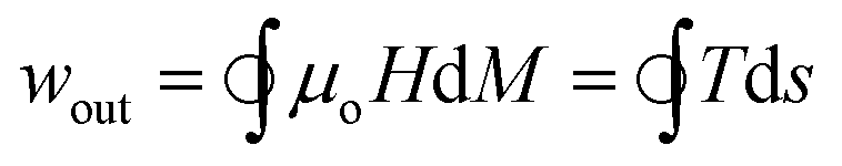
According to the first law of thermodynamics, the change in the internal energy du for a unit mass of a closed thermodynamic system is given by| du = δq − δw | (1) |
| δq = Tds | (2) |
| δw = μoHdM | (3) |
In eqn (3), only magnetic work has been considered and any other types of work, such as pressure related work (Pdv), have been ignored.
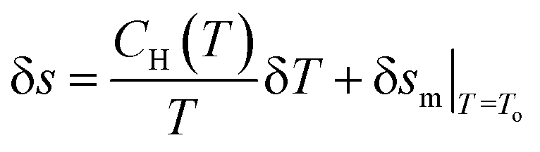
The entropy s of a magnetic material in eqn (2) is the result of the combined effect of magnetic entropy sm (related to the ordering of the spin of the molecules), lattice entropy sl (related to the vibrations of the molecules in the crystal lattice), and electronic entropy se (related to the kinetics of free electrons). Out of the three components, only magnetic entropy sm is influenced by the magnetic field. The external magnetic field forces the molecular spins to orient themselves in one direction, increases the spin ordering, i.e. magnetization, and lowers the system's magnetic entropy. Heating, on the other hand, has a positive effect on all three kinds of entropies. Higher temperature results in larger thermal agitation at the molecular level, promotes disordering, and increases the system's entropy.
| s(T, μoH) = sm(T, μoH) + sl(T) + se(T) | (4) |
Fig. 1(a) shows the typical T–s diagram in the vicinity of the Curie temperature for an MCM undergoing the second-order phase transition. For an isothermal process, increasing the magnetic field has no effect on lattice and electronic entropies whereas the magnetic entropy decreases, i.e. δsl|T=To = 0 = δse|T=To and δs|T=To = δsm|T=To < 0. In addition, it is known from the basic thermodynamics that the net entropy of a system changes only by virtue of heat interaction; therefore, for an adiabatic process, increasing the magnetic field should have no net effect on the total entropy of the magnetic material, i.e. δs|ad = 0. However, as explained earlier, the magnetic entropy decreases with increasing applied magnetic field, i.e. δsm|ad < 0. This implies that the entropy change for an adiabatic process is internally adjusted to cancel out the net effect. In fact, when an external magnetic field is applied adiabatically, the magnetic disorder decreases causing the material to release some of its internal energy in the form of thermal energy, called the heat of magnetization. The heat of magnetization is absorbed by the molecules in the crystal lattice and by the free electrons, and therefore the lattice and electronic entropies increase so that δsl|ad + δse|ad = −δsm|ad. Besides, the heat of magnetization increases the temperature of the material by an amount δTad, called the change in adiabatic temperature.
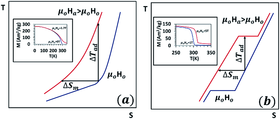 | ||
| Fig. 1 T–s diagram in the vicinity of the Curie temperature for magnetocaloric materials undergoing a second-order phase transition (a) and first-order phase transition (b). Inset shows the magnetization curves for gadolinium (second-order transition) (a) and MnFeP0.8Ge0.2 (first-order transition) (b). Data taken from ref. 21 and 28. | ||
Fig. 1(b) shows the T–s diagram for an MCM undergoing a first-order phase transition near its critical temperature. In contrast to the second-order transition, which is gradual from one phase to another without the coexistence of multiple phases, the first order transition involves the occurrence of two phases in equilibrium in the transition zone. When a material with a first-order transition is heated, it exhibits an abrupt phase change that transforms it from a strongly magnetic to a weakly magnetic phase. The effect is also evident in the magnetization curves for gadolinium (second-order transition) shown in the inset of Fig. 1(a)21 and MnFeP0.8Ge0.2 (first-order transition) shown in the inset of Fig. 1(b).28 For the first-order phase change materials, both the curves, magnetization as well as entropy, show a discontinuity at the transition temperature. Applying an external magnetic field increases the transition temperature because it favours the phase with higher magnetization.29 Besides, the relations δs|T=To = δsm|T=To < 0 for an isothermal process and δsl|ad + δse|ad = −δsm|ad for an adiabatic process apply for first-order and second-order transitions.
Thermomagnetic energy harvester and reverse magnetocaloric cycle
Fig. 2 shows the working principle of a simplified thermal energy harvester based on the reverse magnetocaloric effect. The device will be referred to as the thermomagnetic energy generator (TMEG) in this paper. As shown in the figure, a TMEG consists of a permanent magnet (or an electromagnet) fixed in contact with a heat source, a magnetocaloric material (MCM) that undergoes the reverse magnetocaloric cycle, and an elastic system such as mechanical springs to restore the natural position. The MCM needs to be chosen such that its Curie temperature lies well between the heat source and heat sink temperature. For the waste heat recovery, the heat source is essentially the body containing or releasing the waste heat and the heat sink can either be a nearby cold body or, in most cases, the ambient atmosphere.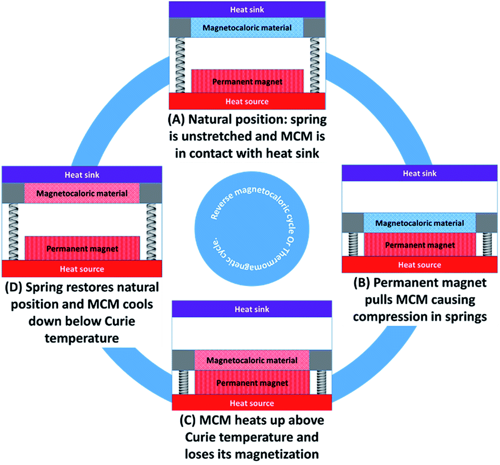 | ||
| Fig. 2 The working principle of a simplified thermomagnetic energy harvester based on the reverse magnetocaloric effect. (A) MCM is at minimum temperature and the highest magnetization. Magnetic force pulls the MCM towards the permanent magnet (B) MCM comes into contact with the heat source and loses its magnetization, (C) spring overcomes the magnetic force and pushes the MCM away, (D) MCM comes into contact with the heat sink, and its magnetization increases with decrease in temperature. | ||
The complete working cycle of a TMEG broadly consists of four key processes, which can be demonstrated using the magnetization vs. magnetic field (M–μoH) plot as shown in Fig. 3(a) or using the temperature vs. entropy (T–s) plot as shown in Fig. 3(b) for a second-order transition magnetocaloric material and in Fig. 3(c) for a first order transition magnetocaloric material.
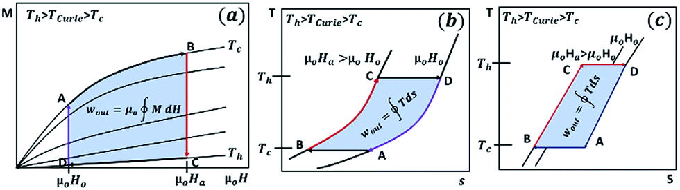 | ||
| Fig. 3 Magnetization vs. magnetic field, (M–μoH) plot (a), temperature vs. entropy (T–s) plot for a second-order transition magnetocaloric material (b), and temperature vs. entropy (T–s) plot for a first order transition magnetocaloric material (c). The direction of the cycles is opposite to that of a magnetocaloric refrigeration cycle; therefore, it can be termed as the reverse magnetocaloric cycle or thermomagnetic cycle. | ||
Process A–B
At the start, in state A, the MCM is cold, and it experiences a weak magnetic field (μoHo). Also, the mechanical springs are unstretched (in practice, a slight compression is needed to create a contact pressure between the MCM and the heat sink. This enhances the heat transfer). The MCM is magnetized, and thus it is attracted by the permanent magnet and as it moves closer to the permanent magnet, it experiences a strong magnetic field (μoHa). Since the movement is small, for an ideal case, it can be assumed that the MCM temperature remains constant (isothermal process). In Fig. 3(a)–(c), process A–B is shown on the isotherm at temperature Tc, where the magnetic field increases from μoHo to μoHa. Process B–C: in state B, the MCM comes into contact with the waste heat source and the heating starts at a constant magnetic field Ha (isofield heating). The magnetic force is highest at the beginning, but it decreases as the MCM temperature rises. However, the magnetic force remains greater than the spring force; therefore, the linear springs are fully compressed. Process B–C is shown on the vertical line at a constant magnetic field μoHa, where the temperature increases from Tc to Th. In Fig. 3(b) and (c), this process is depicted on the isofield curve at μoHa.Process C–D
In state C, the MCM remains in contact with the heat source. As its temperature rises, it loses its magnetization, and eventually, the spring force exceeds the magnetic force between the MCM and the permanent magnet. Restoration starts and the MCM is pushed away. As it moves, its temperature remains roughly constant and therefore, the process can be idealized as an isothermal process before it comes into contact with the heat sink. In Fig. 3(a)–(c), this process is shown on the isotherm at temperature Th, where the magnetic field decreases from μoHa to μoHo.Process D–A
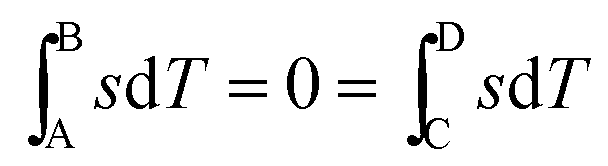
In state D, the MCM comes into contact with the heat sink and the cooling starts at a constant magnetic field μoHo (isofield cooling). As the temperature of the MCM decreases, it regains its magnetization, and eventually, the magnetic force exceeds the spring force. Process D–A is shown on the vertical line at a constant magnetic field μoHo, where the temperature decreases from Th to Tc. In Fig. 3(b) and (c), this process is depicted on the isofield curve at μoHa. Clearly, the direction of the cycles shown in Fig. 3(a)–(c) is opposite to that of a magnetocaloric refrigeration cycle. The cycle, therefore, can be termed as the reverse magnetocaloric cycle or thermomagnetic cycle. Since, for a cyclic process, the net change in the internal energy is zero, eqn (1) can be modified as: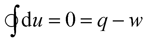 | (5) |
Using eqn (2) and (3), we can derive the specific work output per cycle as:
 | (6) |
It should be noted that the TMEG described in this section relies on the linear motion of the MCM. Therefore, this system can be directly used as a mechanical actuator or as a suitable mechanical-to-electrical energy conversion system by coupling with linear electromagnetic alternator or piezoelectric device to generate electricity.
Methodology for performance calculation
Traditionally, the performance of magnetic refrigerants is measured in terms of the magnetic entropy change (δsm) and adiabatic temperature change (δTad). The performance of a heat engine, however, needs to be described in terms of work output per cycle (wout) and the thermodynamic efficiency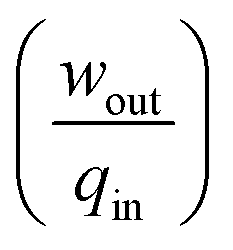 . These variables are interrelated but require some mathematics to deduce the relationship. As shown in eqn (4), the total specific entropy of an MCM is a function of the applied magnetic field and its temperature, i.e. s = s(T, μoH). Therefore, the change in total specific entropy can be expressed as:
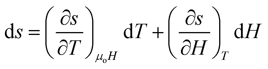 | (7) |
The first partial derivative,  can be defined in terms of specific heat capacity at a constant magnetic field (CH) as
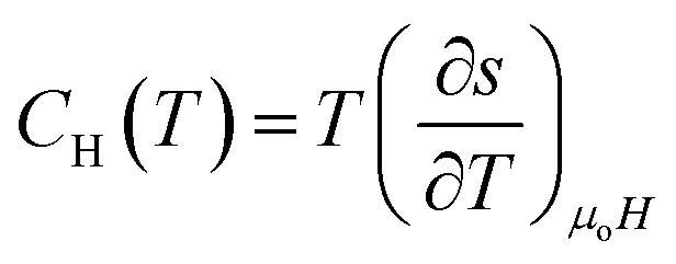 | (8) |
For a small change, δ, the derivatives 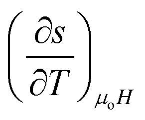 and
and 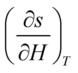 can be approximated as
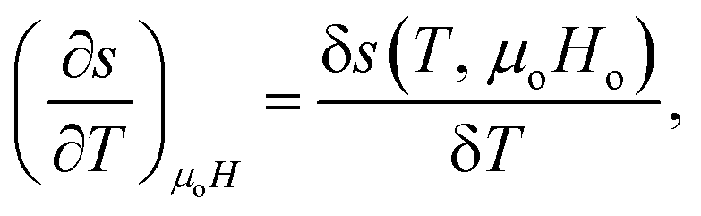 | (9) |
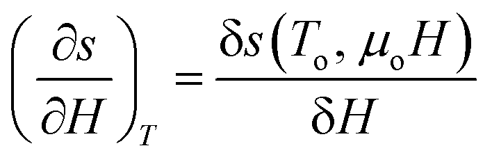 | (10) |
The term δs(To, μoH) in eqn (9) signifies the change in total entropy at a fixed temperature To and is equal to the isothermal change in magnetic entropy δsm|T=To. Eqn (7) can now be simplified as
 | (11) |
For an adiabatic process, δs = 0 and δT = δTad, and therefore
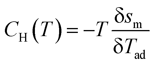 | (12) |
For the reverse magnetocaloric cycle ABCD, described in the previous section, the specific work output per cycle can be given as
 | (13) |
Processes A–B and C–D are isothermal processes, and therefore
 | (14) |
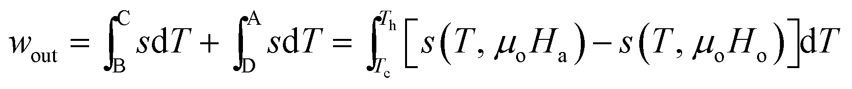 | (15) |
Since [s(T, μoHa) − s(T, μoHo)] = δsm < 0,
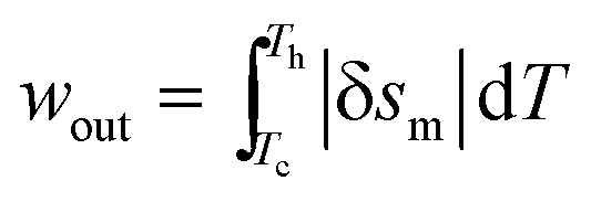 | (16) |
Also, the heat input per cycle qin is given as
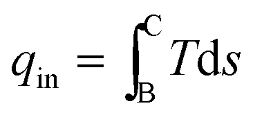 | (17) |
Using eqn (10),
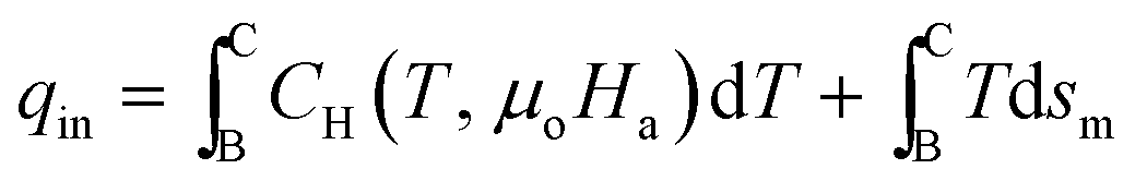 | (18) |
At low applied magnetic fields (μoHa < 2 T), the second term 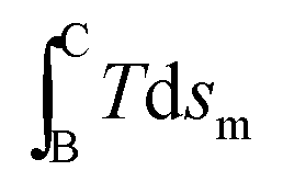 is negligible in comparison to the first term
  .26Eqn (18) can thus be approximated as
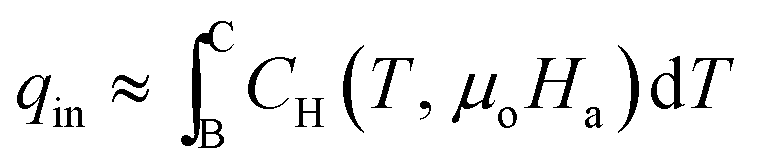 | (19) |
The thermodynamic efficiency of the energy harvester can be calculated using the equation:
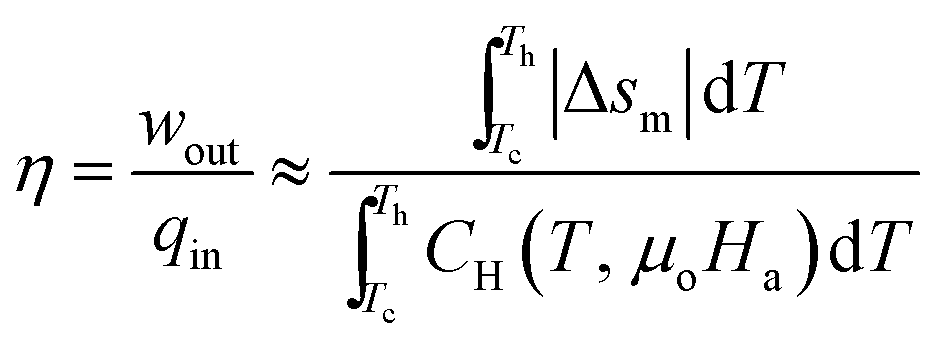 | (20) |
The relative efficiency can also be defined using the absolute thermodynamic efficiency and Carnot efficiency as:
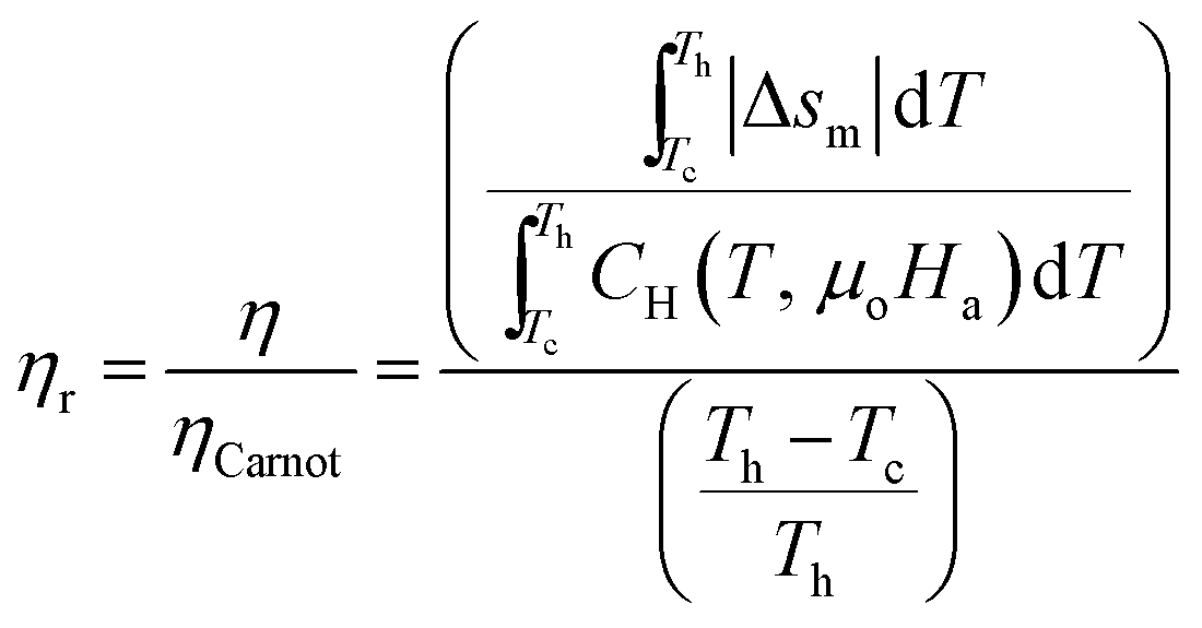 | (21) |
It should be noted that the working principle presented in Fig. 2 and 3 is based on the non-recuperative thermal cycle. This implies that the heat source and heat sink work independently, which is normally the case. However, since the efficiency of TMEGs is normally low, only a small portion of energy from the heat source is utilized into useful work while the majority is rejected to the heat sink. Whenever possible, the efficiency of TMEGs can be improved by using a regenerator. The regenerator temporarily stores the sensible heat rejected during the cooling portion of the thermomagnetic cycle and uses it during the heating cycle. If qr is regenerative heat, the net heat transfer, qh, from the heat source is given as: qh = qin − qr. The enhanced efficiency of a TMEG with a regenerator can be given as:
 | (22) |
The regenerator, however, is expensive and makes the system bulky. Therefore, it should be used only when it is justifiable and cost-effective. For remaining discussion in this study, we have considered the non-recuperative thermal cycle and have used eqn (20) and (21) for calculating the efficiency.
Results and discussion
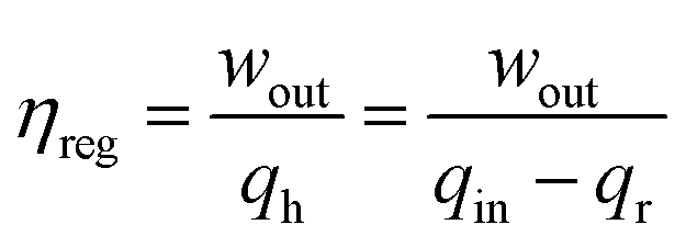
The characteristic eqn (16) and (20), for a thermomagnetic energy harvester, are derived using numerical approximations; therefore, the first and foremost step is to validate these equations using alternative methods. Fig. 4(a) shows the experimental isothermal magnetization curves for gadolinium at two different temperatures, 278 K and 324 K (data taken from ref. 30). As shown in the figure, the area of the shaded region between the curves represents the magnetic work per unit mass, the wout of Gd thermo-magnetically cycled between the temperatures 278 K and 324 K and magnetic fields 0 T and 2 T. Fig. 4(b) shows the δsmvs. T plot for Gd for the change in the magnetic field of 0–2 T.30 With the help of Fig. 4(c), it can be explained that the area of the shaded region under the δsm curve is approximately equal to the specific work per cycle, wout. wout values obtained from the two methods are 287.6 J kg−1 and 225.3 J kg−1 respectively. Fig. 4(e) shows the experimental specific heat capacity, CH,30 at a constant magnetic field of 2 T and the same parameter obtained from eqn (12) using δsm data given in Fig. 4(b) and δTad data from Fig. 4(d). It can be seen that both eqn (11) and (16) are conservative and under-predict the values. However, the difference in thermodynamic efficiency obtained using the two methods is found to be less than 10%.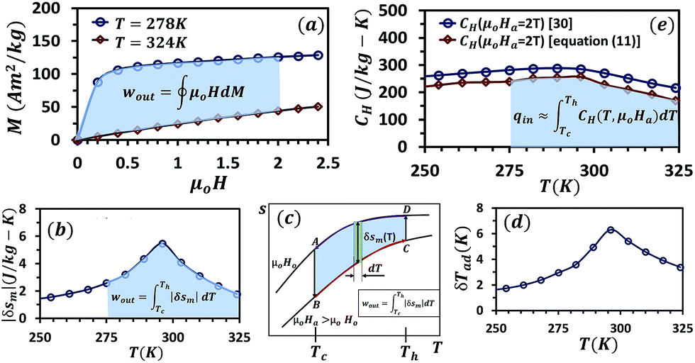 | ||
Fig. 4 The experimental isothermal magnetization curves for gadolinium at two different temperatures, 278 K and 324 K (a). The area of the shaded region between the curves represents wout of Gd at 278–324 K and 0–2 T. δsmvs. T plot for Gd for the magnetic field change of 0–2 T (b). The area bounded between two magnetic field curves and between two temperatures represents wout per cycle and it can be approximated as  (c). δTadvs. T plot for Gd for the magnetic field change of 0–2 T (d). The experimental specific heat capacity, CH at a constant magnetic field of 2 T and the same parameter obtained from eqn (12) (e). Data taken from ref. 30. (c). δTadvs. T plot for Gd for the magnetic field change of 0–2 T (d). The experimental specific heat capacity, CH at a constant magnetic field of 2 T and the same parameter obtained from eqn (12) (e). Data taken from ref. 30. | ||
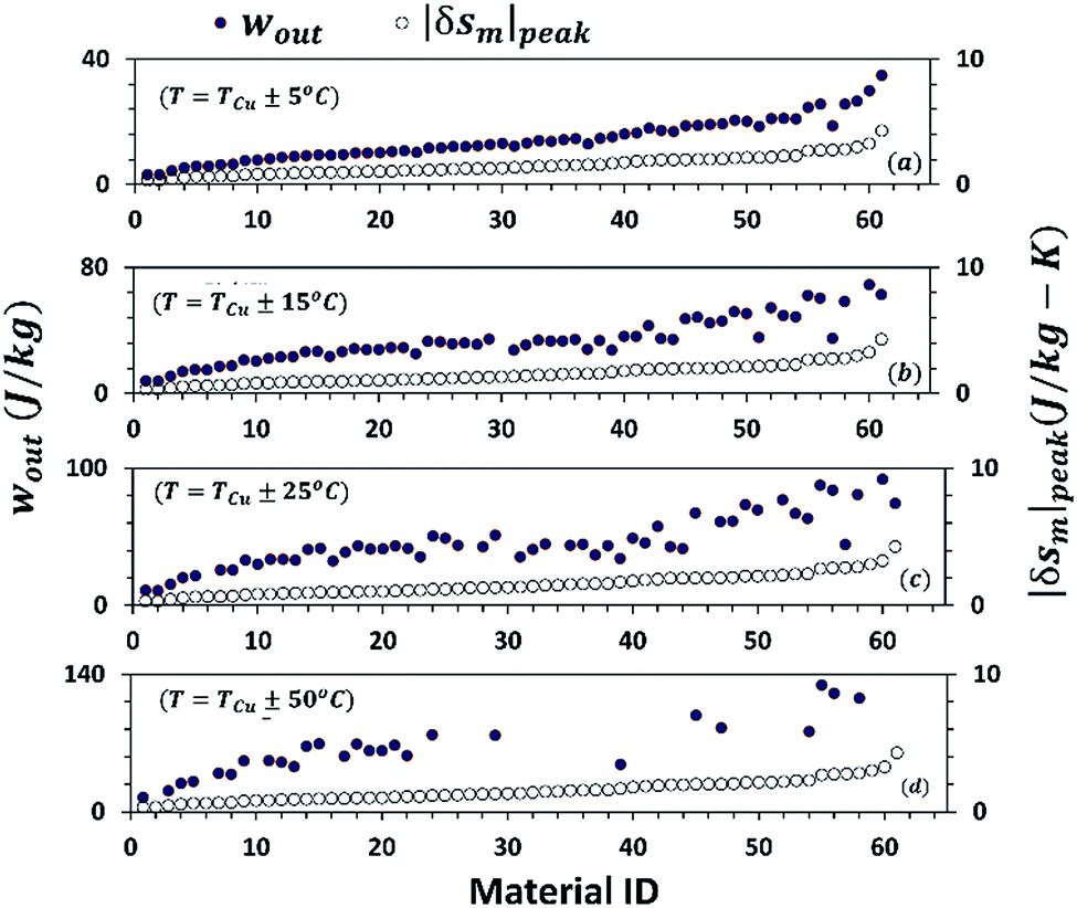
Table 1 shows the list of more than 60 MCMs that have a Curie temperature above 293 K. Information is compiled from ref. 31–53. Each material has been assigned an identification number (ID) for brevity and ease of representation in the figures. Materials have been arranged in increasing order of their maximum magnetic entropy change, |δsm|peak reported in the literature. Fig. 5(a)–(d) demonstrate the maximum change in magnetic entropy |δsm|peak (on the secondary y-axis) and the specific work output per cycle, wout (on the primary y-axis) calculated using eqn (16) for different MCMs operating under various temperature conditions. It should be noted that both the variables increase with increase in the change in the magnetic field, (μoHo − μoHa). The value of μoHo − μoHa taken for this study is 0–1 T. For a few materials, the |δsm| curve was not readily available between 0–1 T in the literature. For such cases, linear interpolation or extrapolation has been used. As shown in Fig. 6(a) and (b), |δsm|peak and wout have a linear relationship with μoHo − μoHa for small changes in the magnetic field. Moreover, it can be observed that wout follows roughly the same trend as |δsm|peak, but this does not necessarily mean that a material with a higher |δsm|peak would provide a higher wout. Some materials such as manganese boride (MnB) has a very sharp |δsm| vs. T curve and therefore its |δsm|peak is larger than the |δsm|peak of Gd. It can be seen in Fig. 5(a)–(d) that the wout of MnB is also greater than that of Gd for the first case, i.e. in a narrow temperature range (T = TCu ± 5 °C). However, in other cases, when the temperature range is large (T = TCu ± 15 °C and T = TCu ± 25 °C), the area under the |δsm| curve of MnB is relatively smaller than the area under the |δsm| curve of Gd, and therefore MnB has a lower wout. This is an important observation because, in the literature, MCMs are often compared in terms of the peak magnetic entropy change |δsm|peak.
| Material | ID | T Cu (K) | Ref. | Material | ID | T Cu (K) | Ref. |
|---|---|---|---|---|---|---|---|
| GdFe6Al6 | 1 | 335 | 31 | Mn0.5Fe0.5B | 32 | 798 | 33 |
| Fe69B12Cr8Gd11 | 2 | 416 | 32 | La0.56Eu0.14Sr0.30MnO3 | 33 | 306 | 42 |
| Fe70B12Cr8Gd10 | 3 | 408 | 32 | La0.7Ca0.2Sr0.1MnO3 | 34 | 312 | 45 |
| Fe72B12Cr8Gd8 | 4 | 410 | 32 | La0.56Er0.14Sr0.30MnO3 | 35 | 331 | 42 |
| Mn0.5Co0.5B | 5 | 411 | 33 | La0.686Er0.014Sr0.30MnO3 | 36 | 348 | 42 |
| La0.5Pb0.5MnO3 | 6 | 350 | 34 | La0.7Ba0.3MnO3 | 37 | 338 | 46 |
| Fe77B12Cr8Gd3 | 7 | 381 | 32 | La0.665Er0.035Sr0.30MnO3 | 38 | 339 | 42 |
| Fe75B12Cr8Gd5 | 8 | 403 | 32 | La0.60Nd0.20Na0.2MnO3 | 39 | 295 | 44 |
| Mn0.4Fe0.6B | 9 | 735 | 33 | La0.7Ca0.06Ba0.24MnO3 | 40 | 317 | 46 |
| La0.5Ca0.3Sr0.2MnO3 | 10 | 318 | 35 | La0.7Ca0.18Ba0.12MnO3 | 41 | 292 | 46 |
| Fe78B12Cr8Gd2 | 11 | 386 | 32 | La0.7Ca0.15Pb0.15MnO3 | 42 | 310 | 47 |
| GdScSi | 12 | 354 | 36 | La0.8Na0.20MnO3 | 43 | 334 | 44 |
| Mn0.6Fe0.4B | 13 | 717 | 33 | La0.75Nd0.05Na0.2MnO3 | 44 | 319 | 44 |
| Fe83Zr6B10Cu1 | 14 | 399 | 37 | La0.6Sr0.2Ca0.2MnO3 | 45 | 335 | 48 |
| Fe82.5Co2.75Ni2.75Zr7B4Cu1 | 15 | 405 | 38 | Gd4Tb1Si4 | 46 | 315 | 49 |
| Mn0.6Co0.4B | 16 | 456 | 33 | La0.835Na0.165MnO3 | 47 | 345 | 50 |
| GdScGe | 17 | 345 | 36 | Gd3Tb2Si4 | 48 | 299 | 49 |
| Fe79B12Cr8Gd | 18 | 360 | 32 | Gd4.5Tb0.5Si4 | 49 | 327 | 49 |
| Fe80.5Nb7B12.5 | 19 | 363 | 40 | La0.65Sr0.35MnO3 | 50 | 305 | 48 |
| Fe81Nb7B12 | 20 | 363 | 39 | La0.70Nd0.10Na0.2MnO3 | 51 | 309 | 44 |
| Fe78Co5Zr6B10Cu1 | 21 | 490 | 37 | Gd5Si4 | 52 | 338 | 49 |
| Mn0.8Co0.2B | 22 | 504 | 33 | Gd3.5Tb1.5Si4 | 53 | 305 | 49 |
| La0.7Pb0.3MnO3 | 23 | 350 | 34 | La0.6Sr0.2Ba0.2MnO3 | 54 | 355 | 48 |
| Fe77Co5.5Ni5.5Zr7B4Cu1 | 24 | 492 | 38 | La2/3Ba1/3MnO2.95 | 55 | 295 | 51 |
| Fe66Co11Ni11Zr7B4Cu1 | 25 | 630 | 38 | La2/3Ba1/3MnO2.98 | 56 | 311 | 51 |
| Mn0.9Co0.1B | 26 | 543 | 33 | La0.7Ca0.1Pb0.2MnO3 | 57 | 328 | 52 |
| La0.845Sr0.155MnO3 | 27 | 315 | 41 | La2/3Ba1/3MnO3 | 58 | 336 | 51 |
| La0.49Er0.21Sr0.30MnO3 | 28 | 311 | 42 | La0.85K0.15MnO3 | 59 | 306 | 53 |
| Fe71.5Co8.25Ni8.25Zr7B4Cu1 | 29 | 571 | 38 | Gd | 60 | 293 | 51 |
| Gd7Pd3 | 30 | 335 | 43 | MnB | 61 | 566 | 33 |
| La0.65Nd0.15Na0.2MnO3 | 31 | 297 | 44 |
 | ||
| Fig. 5 Specific work output per cycle, wout (on the primary y-axis) and peak magnetic entropy change |δsm|peak (on the secondary y-axis) for different MCMs calculated using eqn (16) under different operating temperature conditions: T = TCu ± 5 °C (a), T = TCu ± 15 °C (b), T = TCu ± 25 °C (c), and T = TCu ± 50 °C (d). The magnetic field change is kept constant: μoHo − μoHa = 0–1 T. The number on the x-axis denotes material ID as given in Table 1. wout follows roughly the same trend as |δsm|peak, but this does not necessarily mean a material with a higher |δsm|peak provides a higher wout. | ||
 | ||
| Fig. 6 Specific work output per cycle, wout (on the primary y-axis) and peak magnetic entropy change |δsm|peak (on the secondary y-axis) vs. change in the magnetic field μoHo (0 T) − μoHa for La0.85K0.15MnO3 (a) and La0.80K0.20MnO3 (b). Information taken from ref. 53. Both, wout and |δsm|peak, have a linear relationship with μoHo − μoHa for small changes in the magnetic field. | ||
The top ten MCMs with the highest specific work potential are Gd5Si4, Gd3.5Tb1.5Si4, La0.6Sr0.2Ba0.2MnO3, La2/3Ba1/3MnO2.95, La2/3Ba1/3MnO2.98, La0.7Ca0.1Pb0.2MnO3, La2/3Ba1/3MnO3, La0.85K0.15MnO3, Gd, and MnB. It is interesting to note that despite several decades of research, gadolinium (Gd) is still amongst the top few MCMs having a Curie temperature above room temperature. It is probably because of the fact that the developments in the field of MCMs have been focused primarily on magnetic refrigeration. Fig. 7 shows wout for the top ten materials under different ΔT with temperature varying equally across the Curie temperature (T = TCu ± ΔT). It is important to note that wout does not increase monotonically with increase in ΔT, rather it tends to saturate. This happens because the magnetic phase change in MCMs occurs in a narrow temperature range. The |δsm| curve normally has a sharp peak and it almost flattens at temperatures far away from the Curie temperature. Increasing the temperature range in such a region would virtually have no effect on the work output. In other words, the reverse magnetocaloric effect is most prominent in a narrow temperature range near the Curie temperature.
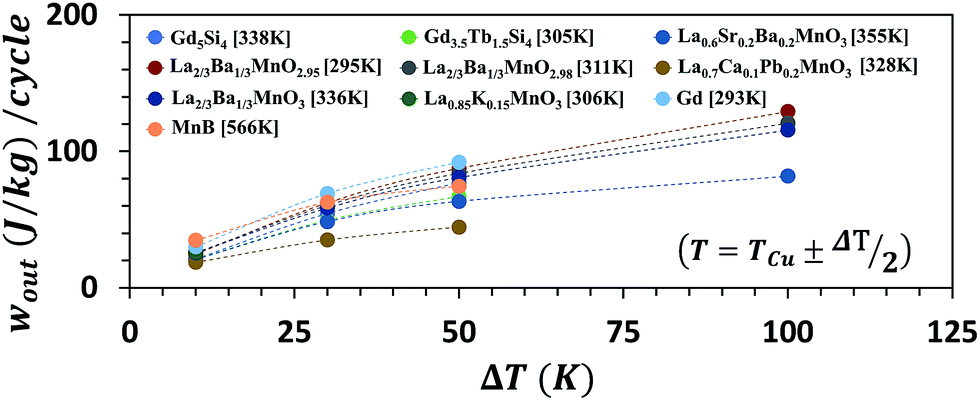 | ||
| Fig. 7 Specific work output per cycle, wout for the top ten materials under different ΔT with temperature varying equally across the Curie temperature (T = TCu ± ΔT). wout saturates when ΔT is large. The reverse magnetocaloric effect is most prominent in a narrow temperature range near the Curie temperature. | ||
Given the fact that a heat source at higher temperature has a higher available energy than the one at lower temperature, it seems more logical to compare the performance of MCMs when the operating temperature is fixed and equal for all the materials, instead of varying the temperature range for different materials as done in Fig. 5(a)–(d). Moreover, for the waste heat recovery, in most cases, the ambient atmosphere acts as the heat sink; therefore, the cold-side temperature needs to be fixed at 25 °C. The work output per cycle for the materials in Table 1 is recalculated under four different fixed temperature conditions: (i) 25–50 °C, (ii) 25–75 °C, (iii) 25–100 °C, and (iv) 25–125 °C. The results are plotted in Fig. 8(a)–(d). Material ID on the abscissa is the same as that indicated in Table 1 and are arranged in increasing order of |δsm|peak. It can be noted that as the temperature increases the plots become sparser. This is because the required material data were not available in the literature at higher temperature for all the materials considered in this study. In Fig. 8(a)–(d), we can see some large variation in wout and clearly higher |δsm|peak does not guarantee a higher |δsm|peak. In the first case, T = 25–50 °C, the top ten performing materials, in increasing order of wout, are Gd, La0.70Nd0.10Na0.2MnO3, Gd4.5Tb0.5Si4, La0.7Ca0.06Ba0.24MnO3, La0.7Ca0.15Pb0.15MnO3, La0.65Sr0.35MnO3, Gd4Tb1Si4, Gd3.5Tb1.5Si4, La0.85K0.15MnO3, and La2/3Ba1/3MnO2.98. The magnitude of wout ranges from 30 J per kg per cycle to 53.5 J per kg per cycle. It increases to about 77 J per kg per cycle at 25–75 °C for La2/3Ba1/3MnO3 (Curie temperature ∼ 63 °C) and La2/3Ba1/3MnO2.98 (Curie temperature ∼ 38 °C). At the heat source temperature of 100 °C, La2/3Ba1/3MnO2.98 shows a working potential of about 87.8 J per kg per cycle. In addition, at T = 25–50 °C, Gd5Si4 (Curie temperature ∼ 65 °C) and La2/3Ba1/3MnO3 can theoretically produce energy up to 100 J per kg per cycle. This implies that a thermomagnetic generator operating at a frequency of 1 rev per s (1 Hz) has the potential to produce a power density of 100 W kg−1. Of course, this is the theoretical limit and an actual device would have several types of losses that need to be accounted for in the analysis, before calculating the final mechanical or electrical power output. There are not many materials for the fourth case: T = 25–125 °C, but La0.835Na0.165MnO3 (Curie temperature ∼ 72 °C) and La0.6Sr0.2Ca0.2MnO3 (Curie temperature ∼ 62 °C) seem to have a specific work potential of 85 J per kg per cycle and 92 J per kg per cycle, respectively.
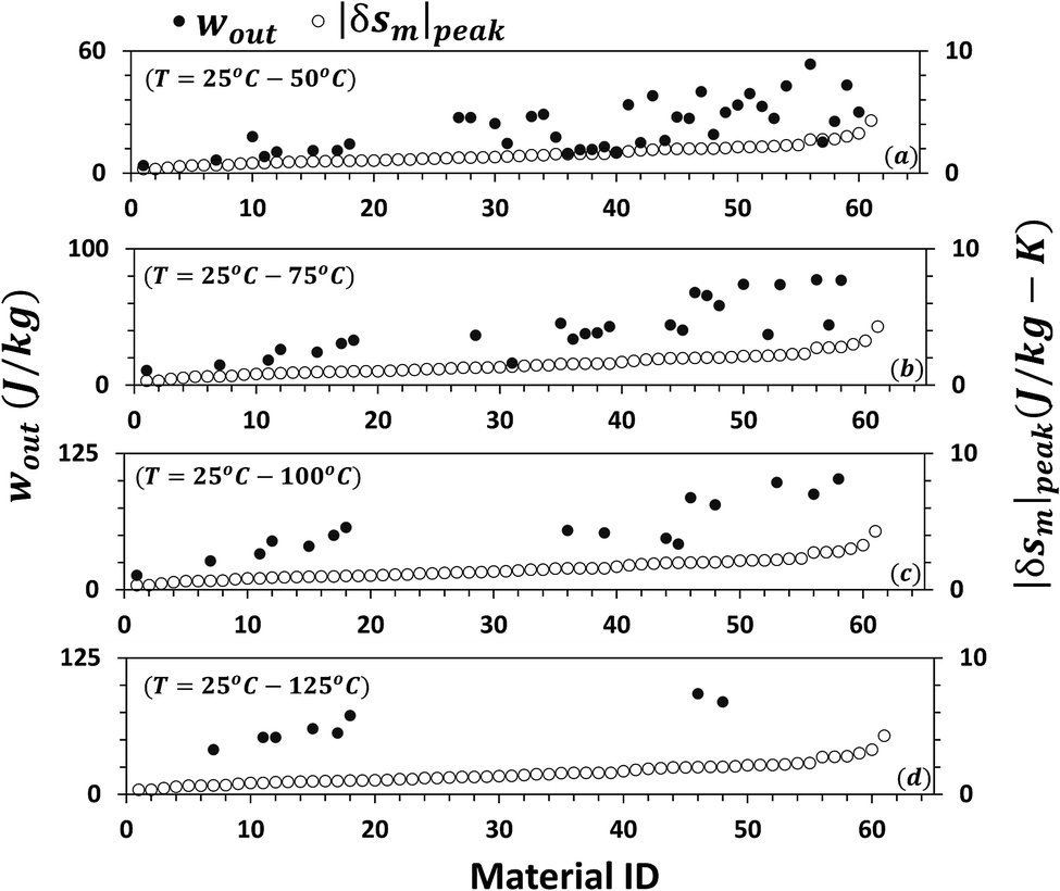 | ||
| Fig. 8 The specific work output per cycle, wout under four different fixed temperature conditions: 25–50 °C (a), 25–75 °C (b), 25–100 °C (c), and 25–125 °C (d). Material ID on the abscissa is the same as that indicated in Table 1. At T = (25–50 °C), the top ten performing materials, in increasing order of wout, are Gd, La0.70Nd0.10Na0.2MnO3, Gd4.5Tb0.5Si4, La0.7Ca0.06Ba0.24MnO3, La0.7Ca0.15Pb0.15MnO3, La0.65Sr0.35MnO3, Gd4Tb1Si4, Gd3.5Tb1.5Si4, La0.85K0.15MnO3, and La2/3Ba1/3MnO2.98. wout ranges from 30 J per kg per cycle to 53.5 J per kg per cycle. wout increases to about 77 J per kg per cycle at 25–75 °C for La2/3Ba1/3MnO3 and La2/3Ba1/3MnO2.98. Increasing the heat source temperature further to 100 °C, Gd5Si4 and La2/3Ba1/3MnO3 can theoretically produce energy up to 100 J per kg per cycle. | ||
From eqn (20) and (21), calculating the thermodynamic efficiency of a material requires knowledge of its heat capacity. The heat capacity of an MCM can be either measured experimentally or approximated using eqn (12), if the adiabatic temperature change δTad is known. Unfortunately, most of the MCMs listed in Table 1 are prototype materials whose δTad has not been reported in papers. Therefore, in this study, we are unable to compare the thermomagnetic efficiency of all the materials. However, in order to provide an estimate of TMEG efficiency, we have compared the thermodynamic efficiency of Gd (second-order MCM) and MnB (first-order MCM) under different ΔT conditions. Fig. 9(a) and (b) show absolute efficiency (calculated using eqn (20)) and relative efficiency (calculated using eqn (21)), respectively. It can be noted that both absolute and relative efficiencies decrease with increase in temperature difference. Gd has more than five times higher absolute efficiency and more than twice relative efficiency than MnB. In addition, when the temperature difference is small (ΔT = 5 °C), the relative efficiency for MnB is 20%, whereas the relative efficiency for Gd reaches as high as 55%, which is in agreement with the analytical results of Elliott.20
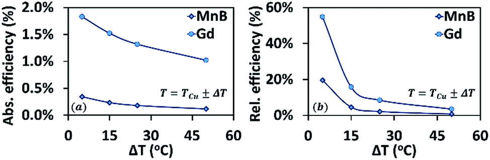 | ||
| Fig. 9 (a) Absolute efficiency and (b) relative efficiency of Gd (second-order MCM) and MnB (first-order MCM) under different ΔT conditions. When the temperature difference is small (ΔT = 5 °C), the relative efficiency for MnB is 20%, whereas the relative efficiency for Gd reaches as high as 55%. | ||
It should be noted that the work output per cycle, presented in this study, is just one of the criteria for the selection of the MCM. There are several other considerations that must be taken into account. For example, most MCMs, especially the ones undergoing the first-order transition, have some thermal and magnetic hysteresis. Large thermal and magnetic hysteresis lowers the energy output and makes the material unsuitable for energy harvesting. For example, MnAs (not included in this study) has |δsm|peak = 27 J kg−1 K−1 at a magnetic field change of 6 T.54 Despite this property, it is not considered a suitable material for the magnetocaloric cycle as the phase change in MnAs is accompanied by a large thermal hysteresis of about 5 K.55 Nearly zero magnetic hysteresis and small thermal hysteresis are positive attributes of a good MCM. In addition, small specific heat and large thermal conductivity ensure rapid heat exchange and temperature change. This implies that, out of two MCMs having the same energy output per cycle, the one with lower specific heat and larger thermal conductivity is expected to have a higher thermomagnetic cycle frequency and thus a higher power output.
Conclusions
In summary, this study investigated the criteria for implementing magnetocaloric materials for harnessing low-grade waste heat (temperature less than 230 °C). Low-grade waste heat is mostly discarded to the atmosphere because of the limitations of current energy harvesting methods. This study analysed the performance of more than 60 magnetocaloric materials for energy harvesting. The specific work output per cycle, wout for different materials was calculated and compared under different operating temperature conditions: first at temperatures varying equally across the Curie temperature and then in fixed temperature ranges. The major findings of the study can be summarized as follows:The peak magnetic entropy change |δsm|peak and the specific work per cycle wout for magnetocaloric materials have a linear relationship with the change in the magnetic field, (μoHo − μoHa) as long as the change is small.
• In the first case, when the temperature was varied as T = TCu ± 5 °C, T = TCu ± 15 °C, T = TCu ± 25 °C, and T = TCu ± 50 °C, gadolinium (Gd) appeared to be the best performing (highest wout) material.
• However, in the second case when the heat sink temperature was fixed at the ambient temperature of 25 °C and the heat source temperature was varied as Th = 50 °C, Th = 75 °C, Th = 100 °C, and Th = 125 °C, gadolinium was not found to be a preferred material for energy harvesting purposes.
• The top five materials for low temperature difference energy harvesting were found to be La0.65Sr0.35MnO3, Gd4Tb1Si4, Gd3.5Tb1.5Si4, La0.85K0.15MnO3, and La2/3Ba1/3MnO2.98.
• La2/3Ba1/3MnO2.98 appeared to be the most promising material with a working potential of 53.5 J per kg per cycle at Th = 50 °C, 77.4 J per kg per cycle at Th = 75 °C, and 87.8 J per kg per cycle at Th = 100 °C.
• A few other materials with a higher Curie temperature, such as Gd5Si4 and La2/3Ba1/3MnO3, were found to have a working potential of about 100 J per kg per cycle at a heat source temperature of 100 °C.
Acknowledgements
The authors acknowledge the financial support from the ICTAS Doctoral Scholars Program (R. K.) and the Office of Basic Energy Science, Department of Energy (S. P.) through grant number DE-FG02-06ER46290.References
- C. Forman, I. K. Muritala, R. Pardemann and B. Meyer, Renewable Sustainable Energy Rev., 2016, 57, 1568–1579 CrossRef.
- Waste Heat Recovery: Technology and Opportunities in U.S. Industry, http://www1.eere.energy.gov/manufacturing/intensiveprocesses/pdfs/waste_heat_recovery.pdf.
- G. Brown, J. Appl. Phys., 1976, 47, 3673–3680 CrossRef CAS.
- J. R. Gómez, R. F. Garcia, A. D. M. Catoira and M. R. Gómez, Renewable Sustainable Energy Rev., 2013, 17, 74–82 CrossRef.
- E. Warburg, Ann. Phys., 1881, 249, 141–164 CrossRef.
- V. K. Pecharsky and K. A. Gschneidner Jr, Phys. Rev. Lett., 1997, 78, 4494 CrossRef CAS.
- E. Brück, O. Tegus, D. C. Thanh and K. Buschow, J. Magn. Magn. Mater., 2007, 310, 2793–2799 CrossRef.
- K. A. Gschneidner Jr, V. Pecharsky and A. Tsokol, Rep. Prog. Phys., 2005, 68, 1479 CrossRef.
- V. K. Pecharsky and K. A. Gschneidner Jr, J. Magn. Magn. Mater., 1999, 200, 44–56 CrossRef CAS.
- M.-H. Phan and S.-C. Yu, J. Magn. Magn. Mater., 2007, 308, 325–340 CrossRef CAS.
- B. Yu, Q. Gao, B. Zhang, X. Meng and Z. Chen, Int. J. Refrig., 2003, 26, 622–636 CrossRef.
- D. Solomon, J. Appl. Phys., 1988, 63, 915–921 CrossRef CAS.
- D. Solomon, J. Appl. Phys., 1989, 65, 3687–3693 CrossRef.
- D. Solomon, Energy Convers. Manage., 1991, 31, 157–173 CrossRef CAS.
- N. Tesla, US Pat., 396121, 1889.
- N. Tesla, US Pat., 428057, 1890.
- T. A. Edison, US Pat., 380100, 1888.
- T. A. Edison, US Pat., 476983, 1892.
- K. E. Bulgrin, Y. S. Ju, G. P. Carman, A. S. Lavine, A coupled thermal and mechanical model of a thermal energy harvesting device, ASME 2009 International Mechanical Engineering Congress and Exposition, American Society of Mechanical Engineers, 2009, pp. 327–335 Search PubMed.
- J. Elliott, J. Appl. Phys., 1959, 30, 1774–1777 CrossRef CAS.
- K. B. Joshi and S. Priya, Smart Mater. Struct., 2013, 22, 055005 CrossRef.
- L. D. Kirol and J. I. Mills, J. Appl. Phys., 1984, 56, 824–828 CrossRef CAS.
- H. Stauss, J. Appl. Phys., 1959, 30, 1622–1623 CrossRef.
- M. Ujihara, G. Carman and D. Lee, Appl. Phys. Lett., 2007, 91, 093508 CrossRef.
- A. Post, C. Knight and E. Kisi, J. Appl. Phys., 2013, 114, 033915 CrossRef.
- C.-J. Hsu, S. M. Sandoval, K. P. Wetzlar and G. P. Carman, J. Appl. Phys., 2011, 110, 123923 CrossRef.
- A. Kitanovski, J. Tušek, U. Tomc, U. Plaznik, M. Ozbolt and A. Poredoš, Magnetocaloric Energy Conversion, Springer International Publishing, 2015, vol. 565, p. 269 Search PubMed.
- L. Caron, Z. Ou, T. Nguyen, D. C. Thanh, O. Tegus and E. Brück, J. Magn. Magn. Mater., 2009, 321, 3559–3566 CrossRef CAS.
- H. E. Karaca, I. Karaman, B. Basaran, Y. Ren, Y. I. Chumlyakov and H. J. Maier, Adv. Funct. Mater., 2009, 19, 983–998 CrossRef CAS.
- S. Y. Dan'Kov, A. Tishin, V. Pecharsky and K. Gschneidner, Phys. Rev. B: Condens. Matter Mater. Phys., 1998, 57, 3478 CrossRef.
- M. Klimczak and E. Talik, J. Phys.: Conf. Ser., 2010, 092009 CrossRef.
- J. Law, R. Ramanujan and V. Franco, J. Alloys Compd., 2010, 508, 14–19 CrossRef CAS.
- M. Fries, Z. Gercsi, S. Ener, K. P. Skokov and O. Gutfleisch, Acta Mater., 2016, 113, 213–220 CrossRef CAS.
- N. Chau, H. N. Nhat, N. H. Luong, D. Le Minh, N. D. Tho and N. N. Chau, Phys. B, 2003, 327, 270–278 CrossRef CAS.
- J. Li, W. Sun, W. Ao and J. Tang, J. Magn. Magn. Mater., 2006, 302, 463–466 CrossRef CAS.
- S. Couillaud, E. Gaudin, V. Franco, A. Conde, R. Pöttgen, B. Heying, U. C. Rodewald and B. Chevalier, Intermetallics, 2011, 19, 1573–1578 CrossRef CAS.
- V. Franco, J. Blázquez and A. Conde, J. Appl. Phys., 2006, 100, 064307 CrossRef.
- R. Caballero-Flores, V. Franco, A. Conde, K. Knipling and M. Willard, Appl. Phys. Lett., 2010, 96, 182506 CrossRef.
- I. Skorvanek and J. Kovac, Czech J. Phys., 2004, 54, 189–192 CrossRef.
- I. Škorvánek, J. Kováč, J. Marcin, P. Švec and D. Janičkovič, Mater. Sci. Eng., A, 2007, 449, 460–463 CrossRef.
- M. H. Phan, T. L. Phan, S. C. Yu, N. D. Tho and N. Chau, Phys. Status Solidi B, 2004, 241, 1744–1747 CrossRef CAS.
- J. Amaral, M. Reis, J. Araujo, P. Tavares and V. Amaral, Development of manganite materials for room-temperature magnetocaloric applications, Proceedings of the First IIF–IIR International Conference on Magnetic Refrigeration at Room Temperature, Montreux, Switzerland, 2005 Search PubMed.
- F. Canepa, M. Napoletano and S. Cirafici, Intermetallics, 2002, 10, 731–734 CrossRef CAS.
- D.-L. Hou, C.-X. Yue, Y. Bai, Q.-H. Liu, X.-Y. Zhao and G.-D. Tang, Solid State Commun., 2006, 140, 459–463 CrossRef CAS.
- W. Sun, J. Li, W. Ao, J. Tang and X. Gong, Powder Technol., 2006, 166, 77–80 CrossRef CAS.
- M.-H. Phan, S.-B. Tian, S.-C. Yu and A. Ulyanov, J. Magn. Magn. Mater., 2003, 256, 306–310 CrossRef CAS.
- D. Hanh, M. Islam, F. Khan, D. Minh and N. Chau, J. Magn. Magn. Mater., 2007, 310, 2826–2828 CrossRef CAS.
- M. Phan, S. Tian, D. Hoang, S. Yu, C. Nguyen and A. Ulyanov, J. Magn. Magn. Mater., 2003, 258, 309–311 CrossRef.
- Y. Spichkin, V. Pecharsky and K. Gschneidner Jr, J. Appl. Phys., 2001, 89, 1738–1745 CrossRef CAS.
- W. Zhong, W. Chen, W. Ding, N. Zhang, Y. Du and Q. Yan, Solid State Commun., 1998, 106, 55–58 CrossRef CAS.
- W. Zhong, W. Chen, C. Au and Y. Du, J. Magn. Magn. Mater., 2003, 261, 238–243 CrossRef CAS.
- M.-H. Phan, H.-X. Peng, S.-C. Yu, N. D. Tho, H. N. Nhat and N. Chau, J. Magn. Magn. Mater., 2007, 316, e562–e565 CrossRef CAS.
- S. Das and T. Dey, J. Alloys Compd., 2007, 440, 30–35 CrossRef CAS.
- M. Liu and B.-f. Yu, J. Cent. South Univ. Technol., 2009, 16, 1–12 CrossRef CAS.
- H. Wada and Y. Tanabe, Appl. Phys. Lett., 2001, 79, 3302–3304 CrossRef CAS.
| This journal is © The Royal Society of Chemistry 2017 |