
 Open Access Article
 This Open Access Article is licensed under a
 Creative Commons Attribution 3.0 Unported Licence
Prediction of supercritical carbon dioxide solubility in polymers based on hybrid artificial intelligence method integrated with the diffusion theory
Li Mengshan *ab,
Liu Lianga,
Huang Xingyuanb,
Liu Heshengb,
Chen Bingshenga,
Guan Lixina and
Wu Yana
*ab,
Liu Lianga,
Huang Xingyuanb,
Liu Heshengb,
Chen Bingshenga,
Guan Lixina and
Wu Yana
aCollege of Physics and Electronic Information, Gannan Normal University, Ganzhou, 341000, Jiangxi, China. E-mail: jcimsli@163.com
bCollege of Mechanical and Electric Engineering, Nanchang University, Nanchang, 333001, Jiangxi, China
First published on 25th October 2017
Abstract
Solubility is one of important research hotspots of physical chemistry properties and is widely utilized in the modification, synthesis and preparation of a lot of materials. To avoid the defects of traditional thermodynamic dissolution forecasting methods, according to the mass transfer features of a two-phase system, the dissolution process is simulated. In this paper, the diffusion theory is integrated into the improvement of particle swarm optimization (PSO) so that the particles in the algorithm evolve along with the diffusion energy. In this way, the improved PSO of dual-population diffusion is obtained and used to train the parameters of the radial basis function artificial neural network. Then, a prediction model for supercritical carbon dioxide solubility in polymers is proposed. The solution experiments of 8 polymers indicate that the predicted values with the model are consistent with the experimental results. The prediction accuracy is higher and the correlation is significant. The average relative error, mean square error and square correlation coefficient are respectively 0.0043, 0.0161, and 0.9954. The prediction model has a high comprehensive performance and provides the basis for the prediction, analysis and optimization of other physical and chemical fields.
1. Introduction
The solubility property of supercritical carbon dioxide (ScCO2) in a polymer is widely utilized in the modification and synthesis of materials, the preparation of new materials, and other fields.1–6 Under the supercritical conditions of high temperature and high pressure, dissolution experiments are characterized by the relatively difficult operation procedure, high cost, long time, and high manpower requirements and it is not easy to get solubility data.7,8 Therefore, it is of great significance to establish the precise dissolution prediction model.9,10The dissolution of ScCO2 in polymers is influenced by many factors, such as temperature, pressure, density and the polarity of polymer molecules. These factors represent the extremely complex nonlinear relationships with the dissolution and are correlated with each other. Therefore, traditional thermodynamic state equation and empirical equation cannot provide the satisfactory prediction accuracy of the solubility.5,11,12 Artificial neural network (ANN) has the better self-organization, tolerance and nonlinear processing abilities, which make it especially suitable for solving the problem of solubility prediction.13–16 Bakhbakhi17 and Lashkarbolooki18 et al. compared the solubility prediction results obtained with ANN and equations of state and indicated that ANN method was superior to the equations of state in the prediction accuracy and correlation. Gharagheizi et al.19 predicted the solubility of various compounds in ScCO2, indicating that the prediction accuracy and correlation of ANN were satisfactory. Eslamimanesh et al.20 indicated that ANN had the superior prediction performance in the solubility experiment of ScCO2. Pahlavanzadeh et al.21 predicted the solubility with ANN and Deshmukh–Mather method and indicated that ANN was superior to the traditional thermodynamic prediction methods.
Prediction reliability and accuracy of ANN depend on its training algorithm for the optimizing the model structure and parameters. Various optimization algorithms had been developed for ANN training. Evolution algorithms are the most widely used,22 including genetic algorithm,23 simulated annealing algorithm, particle swarm optimization algorithm (PSO),24–26 and ant colony algorithm.27 Liu et al.28 used the PSO algorithm and online strategy to train the fuzzy neural network and successfully predicted the melt index. Lazzus et al.29 precisely predicted the phase equilibrium data of ScCO2 with PSO algorithm. The solubility prediction method of radial basis function artificial neural network and adaptive fuzzy nervous system proposed by Khajeh et al.30 is superior to the traditional method in prediction accuracy and correlation. Hussain et al.31 proposed the mixed neural network solution calculation model by combining Kent–Eisenberg with ANN and realized the better prediction performance. Li et al.32–38 also proposed several dissolution prediction models by combining chaos theory and particle swarm algorithm with the clustering method, improved the ANN training algorithm, and obtained the better prediction accuracy and correlation.
The above research focuses on the improvement in the model method itself, but the essence of the dissolution process is not considered. In the static condition, the essence of dissolution is the diffusion process of the solute molecules adsorbed on the surface to the solvent. The diffusion process is a mass transfer phenomenon under the thermal motion of molecules. The mass transfer is caused by the difference in density or temperature of the two-phase medium. Molecules move from the medium phase with the larger density to the medium phase with the smaller density until the equilibrium state is reached. In the polymer/ScCO2 two-phase system, due to the interface force, CO2 molecules are adsorbed on the interfacial film layer and diffused to the lining of the interfacial membrane. CO2 molecules into the membrane layer are dissolved in the polymer melt. At present, the PSO algorithm based on the migration idea is seldom used in practical problems, especially in the field of thermodynamics. In the study, we attempted to improve the PSO algorithm in two aspects. Firstly, particles in PSO algorithm are similar to the dissolved molecules in the dissolution process and the similarity is mainly reflected by endowing particles in algorithm with the related properties of the dissolved molecules. Secondly, the essence of dissolution is the mass transfer, which is closely correlated with the diffusion theory. Inspired by the diffusion theory, dissolution theory and particle evolution algorithm, we found that the trajectory of CO2 molecules in the diffusion process could be simulated by the motion of particles in the evolution algorithm. Therefore, we integrated the diffusion theory with the improvement of PSO algorithm and effectively simulated the dissolution process of ScCO2 in polymers. With the improved PSO algorithm based on diffusion theory, we performed ANN training and obtained the hybrid intelligent prediction model for the solubility of ScCO2 in polymers.
2. Model theory
2.1 Particle swarm optimization
PSO algorithm is a group evolution algorithm put forward by Eberhart and Kennedy39 based on the social behaviors of birds. In the iterative process of PSO algorithm, it is assumed that in an n-dimensional search space, the particle population X = (x1,x2,…,xn)T is composed of m particles. The position of the ith particle is denoted as xi = (xi,1,xi,2,…,xi,n)T and the velocity of the ith particle is expressed as vi = (vi,1,vi,2,…,vi,n)T. Particles use individual extremum and global extremum to save the particle's own best position and particle population's best position. The formula is expressed as follows:| vi,dk+1 = ωvi,dk + c1(pi,dk − xi,dk) + c2(pg,dk − xi,dk) | (1) |
| xi,dk+1 = xi,dk + vi,dk+1 | (2) |
2.2 Double-population particle swarm optimization (PSO) algorithm based on the diffusion theory
In PSO, particle is designed as a potential solution in search space. A particle updates its speed and position through an iterative formula. In the ScCO2/polymer solution system, there are two-phase molecular systems of ScCO2 and polymer melt. According to the diffusion theory, the energy indicating the process that molecules overcome their barrier to diffuse from their original positions to other positions is called diffusion energy. In other words, the molecules migrate through the diffusion energy and achieve the mass transfer. The magnitude of the diffusion energy is proportional to the square of the movement velocity of the molecule. However, the speed mainly depends on the temperature of the system. For molecule systems, temperature is a statistic index representing the average kinetic energy of the molecules and it is related to the velocity of the molecules. The faster the molecules move, the higher the temperature is.Inspired by the nature of thermodynamics diffusion and dissolution, in this paper, a double population particle swarm algorithm based on diffusion theory (hereafter referred to as DP-DT-PSO algorithm for short) is proposed. In the DP-DT-PSO algorithm, the velocity of the molecule is substituted for the velocity of the particle, thus simulating the effect of the molecular force field. The diffusion temperature is a statistic index collectively representing the thermal motion of a large number of molecules. In the study on dissolution behaviors, temperature is one of the key influencing factors. It is assumed that there is a population temperature in the particle system reflecting the average temperature of the molecular system during the diffusion process. Before the discussion on the algorithm, several concepts of particle diffusion energy, center of mass of a population, distance of center of mass, and diffusion probability are introduced.
(1) Particle diffusion energy. Objects in motion have kinetic energy. The magnitude of the kinetic energy E is related to the mass and velocity of the object. The calculation formula is provided as follows:
 | (3) |
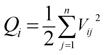 | (4) |
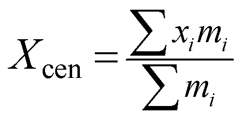
(2) Center of mass of a population. The algorithm converges with the probability of 100% when particles are moving toward a center.40 In order to ensure the convergence of the algorithm, it is assumed that there is a center in the whole population and that all the particles travel to the center in a certain way. Center of mass of a population is a hypothetical point of a population and all the particles in the population approximate the center of mass of a population. The center of mass of a population Xcen is defined as follows:
 | (5) |
(3) Distance of center of mass. In order to describe the positional relationship between the particle and the center of mass of a population, the distance of center of mass di is defined as the distance between the particle and the center of mass of a population:
| di = |xi − Xcen| | (6) |
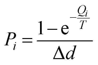
(4) Particle diffusion probability. When a particle meets the diffusion conditions, it does not necessarily generate effective diffusion. The diffusion probability of a particle reflects its diffusion capability or efficiency. The diffusion probability of particles is related to the diffusion energy and the temperature of the population. The diffusion probability Pi is defined as:
 | (7) |
| Δd = ||xi − XAcen| − |xi − XBcen|| | (8) |
In the same temperature system, the diffusion probability of particles is determined by the diffusion energy of particles and the distance difference among the populations. If the higher diffusion energy of particles and the smaller distance difference mean the large diffusion probability of particles.
In the iteration of DP-DT-PSO, the diffusion energy of particles can be firstly obtained by calculating the velocity of each particle in population A (or B). According to the formula of diffusion probability, the diffusion probability value of each particle is calculated. For population A (or B), if the diffusion probability of particles is larger, then the particle is copied to the candidate population of population A (or B). We select the particle with the maximum diffusion probability from the candidate population of population A (or B) to replace the particle with the worst adaptive value in population B (or A). In this way, the sharing of information is realized. Finally, the global extreme value is updated. The implementation process of DP-DT-PSO algorithm is described as follows:
Step 1: initialization of the algorithm.
Two populations (A and B) are initialized to set the number of particles in the two populations, population specification, the position and velocity of all the particles, etc.;
Step 2: calculation of adaptive value.
The adaptive values of all particles are calculated according to the adaptive value function and evaluate the current performance of each particle;
Step 3: extremum updating.
To update the individual extremum of all particles and the global extreme of the two populations;
Step 4: condition judgment.
To determine whether the convergence accuracy meets the requirements or the maximum number of iterations is achieved. If the requirements are met or the maximum number of iterations is achieved, then go to Step 11; otherwise, go to Step 5.
Step 5: calculation of the diffusion probability of particles.
To calculate the diffusion probability Pi of all particles;
Step 6: generation of the candidate population.
For all the particles in population A, the following operation is performed:
For (i = 1; i < M; i++){if (Pi > rand()) copy the particle i to the candidate population TA;}
For population A, the following operation is performed:
For (i = 1; i < M; i++){if (Pi > rand()) copy the particle i to the candidate population TB;}
Step 7: information sharing among populations for simulation particle diffusion.
For population A, the particle with maximum diffusion probability is selected from the candidate population TA to replace the particle with the worst adaptation value in population B. For population B, the particle with maximum diffusion probability is selected from the candidate population TB to replace the particle with the worst adaptation value in population A. If the number of particles in the candidate population is insufficient, return the actual number;
Step 8: global extreme updating.
If the adaptive value of the particles returned from the candidate population is better than the global extremum of the population, the returned particles are used as global extremum, otherwise it is not updated;
Step 9: to save the results obtained in the process.
Return parameters such as the global extremum and local extremum of populations A and B in this iteration, and save them;
Step 10: iterative updating.
Update the formula according to velocity and location, update the velocity and position of the particles in population A/B;
Step 11: to save the results.
To determine whether the results are met. If the results are met, save the results, otherwise jump to Step 2.
2.3 Artificial neural network model based on DP-DT-PSO algorithm
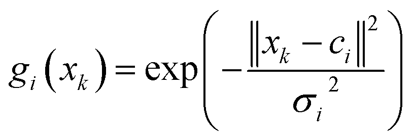
Radial basis function artificial neural network (RBF ANN) is one of the most popular network models and consists of an input layer, an implicit layer, and an output layer. The activation function is a Gaussian function and defined as follows:
 | (9) |
 | (10) |
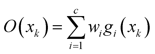
The training process of RBF ANN is mainly to optimize the basis function center, the expansion constant and the connection weights. Through iteration of the three parameters ci,σi,wi, the network is trained. The output of RBF ANN network can be defined as:
| y = f(wh,o,σh,o,ci) | (11) |
| p(i) = [wh,o,σh,o,ci] | (12) |
After RBF ANN is trained by DP-DT-PSO algorithm RBF ANN, a prediction model (DP-DT-PSO RBF ANN) is obtained for the subsequent solution prediction experiment.
3. Model building
3.1 Experimental data
In this paper, 8 kinds of polymers commonly used in industrial production are explored and 327 sets of related data constitute the model database. The source statistics are provided in Table 1.| Polymer | T (K) | P (MPa) | Solubility (g g−1) | Data points | References |
|---|---|---|---|---|---|
| a Polypropylene.b Poly(L-lactide).c High-density polyethylene.d Carboxylated polyesters.e Polystyrene.f Poly(butylene succinate).g Poly(butylene succinate-co-adipate).h Poly(D,L-lactide-co-glycolide). | |||||
| PPa | 313.20–483.70 | 7.400–24.910 | 0.03950–0.26170 | 67 | 41–44 |
| PLLAb | 308.00–323.00 | 9.620–31.460 | 0.16520–0.43010 | 27 | 45 |
| HDPEc | 433.15–473.20 | 10.731–18.123 | 0.00551–0.12296 | 20 | 41 and 42 |
| CPEsd | 306.00–344.00 | 10.150–31.020 | 0.09840–0.63660 | 56 | 46 |
| PSe | 338.22–473.15 | 7.540–44.410 | 0.02641–0.16056 | 70 | 41 and 47–49 |
| PBSf | 323.15–453.15 | 8.008–20.144 | 0.04534–0.17610 | 31 | 41 and 50 |
| PBSAg | 323.15–453.16 | 7.870–20.128 | 0.04763–0.17411 | 29 | 41 and 50 |
| PLGAh | 308.00–323.00 | 10.140–31.470 | 0.09030–0.29630 | 27 | 45 |
| Total | 306.00–483.70 | 7.400–44.410 | 0.00551–0.63660 | 327 | |
According to the types of polymer, the database is subdivided three sets: the training set, validation set and test set. The data of training set are used to train the model. The purpose of the training is to learn all the data, find out the rules among the sample data, and save the rules with parameters such as weights and bias. The data of the validation set is used to verify and subtly correct the trained model so that the model is more accurate. The data of the test set is used to test the predicted performance of the model. The test results directly reflect the advantages and disadvantages of model. For the purpose of more effectively utilizing the data, the data proportions of training set, validation set and test set are respectively 70%, 15%, and 15%. Table 2 shows the data distribution statistics of various polymers.
| Polymer | Training set | Validation set | Testing set | Total |
|---|---|---|---|---|
| PP | 47 | 10 | 10 | 67 |
| PLLA | 19 | 4 | 4 | 27 |
| HDPE | 14 | 3 | 3 | 20 |
| CPEs | 38 | 9 | 9 | 56 |
| PS | 50 | 10 | 10 | 70 |
| PBS | 21 | 5 | 5 | 31 |
| PBSA | 21 | 4 | 4 | 29 |
| PLGA | 19 | 4 | 4 | 27 |
3.2 Model evaluation indexes
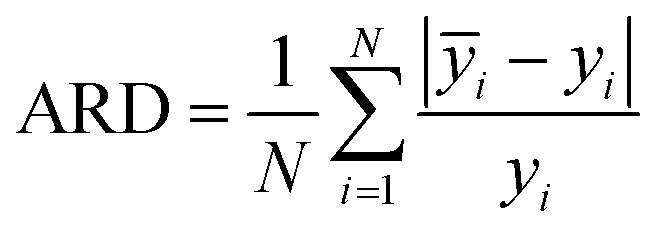
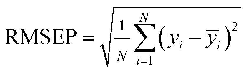
In this paper, measures the prediction performance of the model is analyzed from the three aspects of prediction accuracy, efficiency and stability. In order to evaluate the prediction accuracy and stability, we adopted the three indexes: average relative deviation (ARD), root mean square error of prediction (RMSEP) and squared correlation coefficient (R2) evaluation, which are respectively defined as:
 | (13) |
 | (14) |
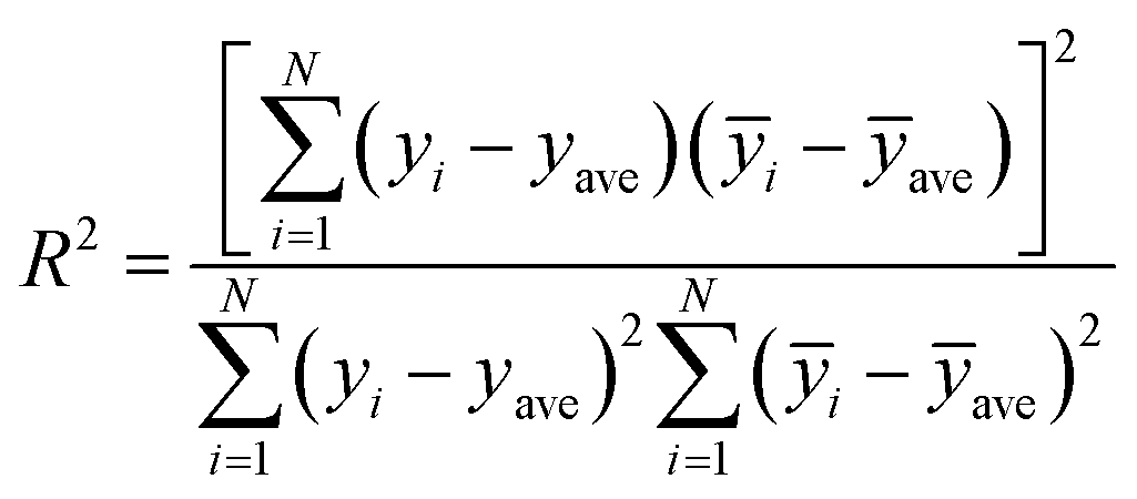 | (15) |
3.3 Model structure
In the three-layer network structure of DP-DT-PSO RBF ANN model, the input layer consists of two nodes respectively indicating the temperature and pressure of the solution system. The number of output layer nodes is 1, representing the solubility of ScCO2 in the polymer. In the hidden layer, this paper adopts the probe method to optimize the number of hidden layer nodes. When the number of nodes is increased from 3 to 13, a total of 11 DP-DT-PSO RBF ANN models are obtained. Fig. 1 illustrates the relationship diagram of the number of hidden layer nodes and the training error (MSE).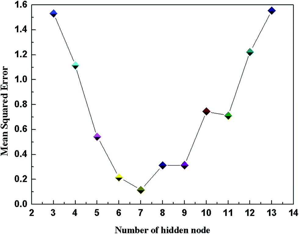 | ||
| Fig. 1 Corrections between the number of hidden node and mean squared error. | ||
In general, the structure with the relatively small error and high correlation coefficient is used as the optimal network structure. As shown in Fig. 1, the hidden layer containing seven neurons is the optimal network structure model.
4. Results and discussion
4.1 Prediction results of the DP-DT-PSO RBF ANN model
Through Matlab 2010a software programming, a 2-7-1 DP-DT-PSO RBF ANN model was established to predict the solubility of supercritical carbon dioxide in 8 polymers. Simulation experiments are performed in Windows 7 SP1 64-bit operating system with 4.00 GB of memory and Intel (R) Core™ i5-4460 processor. Fig. 2 shows the correlation between the predicted values and the experimental values in the training set.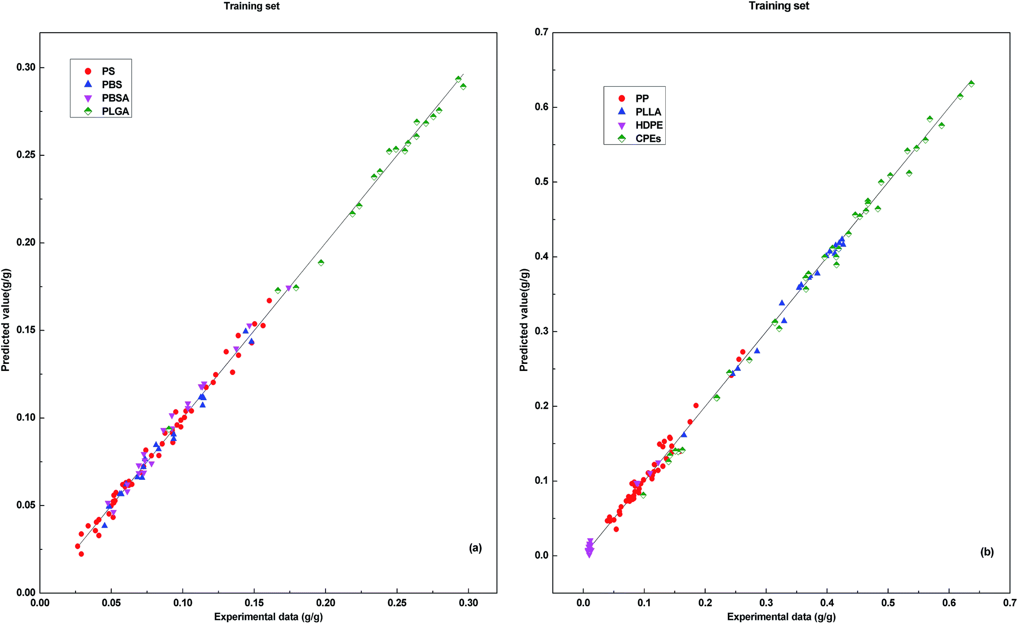 | ||
| Fig. 2 Correlations between the prediction results and experimental data for training set. | ||
The vertical distance between the predicted data points and the line indicates the size of the prediction error. The predicted data points are basically distributed in the vicinity of the line. In the data prediction with the training set, DP-DT-PSO RBF ANN model shows the good performance and the correlation between the predicted value and the experimental value is high. Fig. 3 shows the relationship between model prediction data points and experimental data. The vertical distance indicates that DP-DT-PSO RBF ANN model has high prediction accuracy and good correlation.
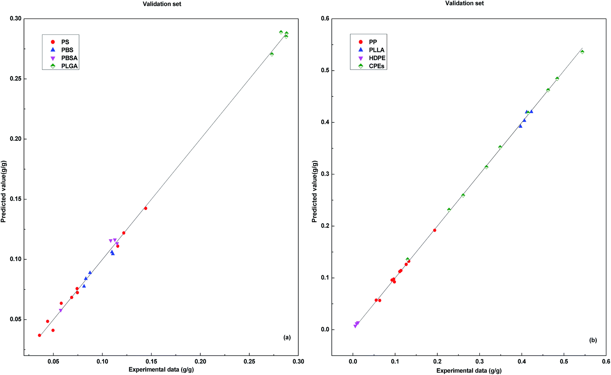 | ||
| Fig. 3 Correlations between the prediction results and experimental data for validation set. | ||
The results of the training set and validation set show that, the performance of model DP-DT-PSO RBF ANN is excellent. The prediction results of the training set indicate the model is well trained. The prediction results of the validation set confirm the reliability of the model. The trained and validated model is applied in the test set. Fig. 4 shows the relationship between the prediction data points and the experimental data points obtained with DP-DT-PSO RBF ANN model in the test set.
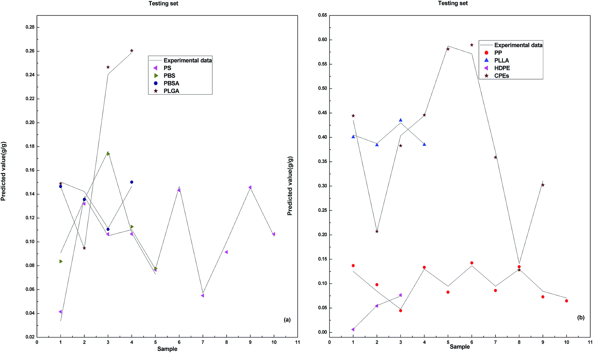 | ||
| Fig. 4 Correlations between the predicted value and experimental data for testing set. | ||
In the test set, the prediction data points of the DP-DT-PSO RBF ANN model are basically distributed in the vicinity of the experimental data points, indicating that the predicted values are close to the experimental values. The distribution of data points of the test set is more dispersed than that of the training set and verification set, indicating that the prediction accuracy of the test set is slightly inferior. Table 3 shows the values of the prediction indexes for each data set.
| Subset | ARD | R2 | RMSEP |
|---|---|---|---|
| Training subset | 0.0038 | 0.9962 | 0.0153 |
| Validation subset | 0.0036 | 0.9967 | 0.0151 |
| Testing subset | 0.0043 | 0.9954 | 0.0161 |
| Average value | 0.0039 | 0.9961 | 0.0155 |
DP-DT-PSO RBF ANN model has the superior performance (including accuracy and correlation) in the training set, validation set, and test set. In the three sets, the validation set shows the better performance: the high prediction accuracy and correlation. The statistical parameters of the model in the prediction experiment for each polymer are provided in Table 4. It is shown that the prediction accuracy of the model in each polymer is almost the same. The correlation between predictive value and experimental value is also better (>0.99). The statistical results verify the better comprehensive generalization ability of the model.
| Polymer | ARD | R2 | RMSEP |
|---|---|---|---|
| PP | 0.0025 | 0.9962 | 0.0158 |
| PLLA | 0.0039 | 0.9959 | 0.0134 |
| HDPE | 0.0048 | 0.9961 | 0.0138 |
| CPEs | 0.0038 | 0.9969 | 0.0161 |
| PS | 0.0039 | 0.9957 | 0.0145 |
| PBS | 0.0048 | 0.9961 | 0.0156 |
| PBSA | 0.0039 | 0.9957 | 0.0214 |
| PLGA | 0.0035 | 0.9961 | 0.0134 |
4.2 Comparative analysis with other models
The above experiments show the good performance of the model DP-DT-PSO RBF ANN in solution prediction. In order to evaluate the performance of DP-DT-PSO RBF ANN model and other models, the three common models, RBF ANN, PSO BP ANN and PSO RBF ANN were respectively used to perform the dissolution prediction for comparison. The running convergence curve of each model is shown in Fig. 5.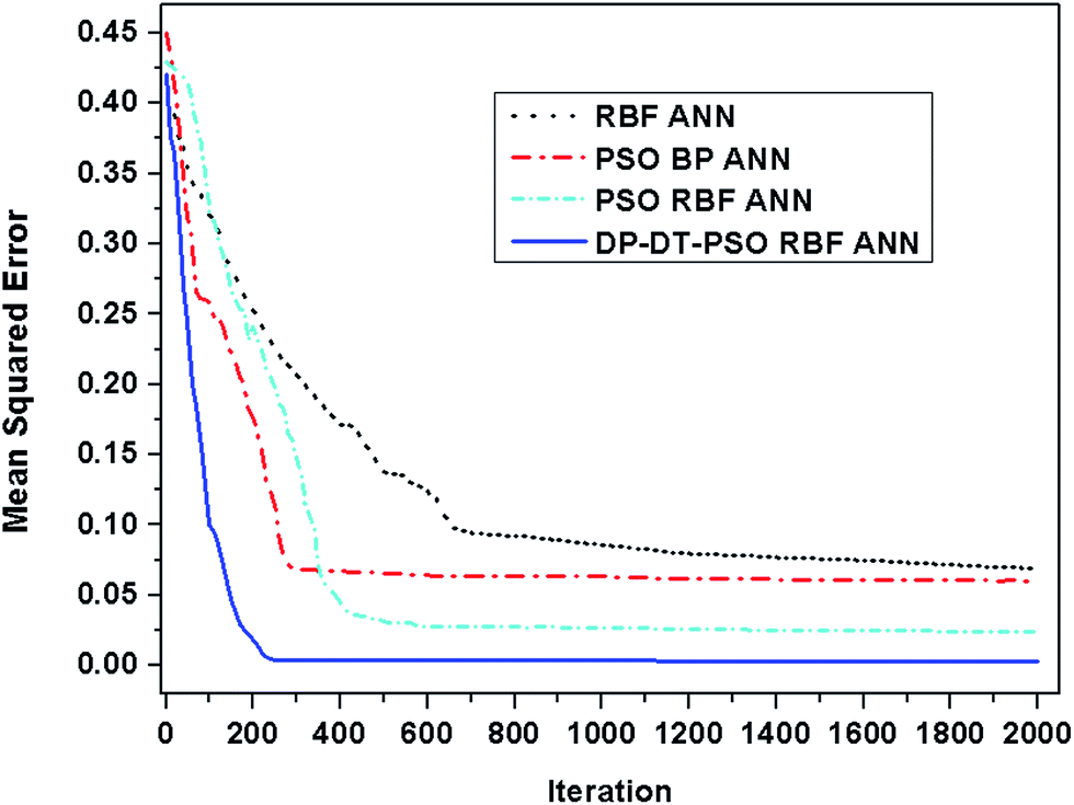 | ||
| Fig. 5 Curve of mean squared error vs. iteration. | ||
The DP-DT-PSO RBF ANN model tends to be stable at nearly 200 iterations, the PSO RBF ANN model tends to be stable at 400 iterations. PSO BP ANN is stable at about 300 iterations. The convergence precision of these models is decreased according to the order: DP-DT-PSO RBF ANN > PSO BP ANN > PSO RBF ANN > RBF ANN. The convergence accuracy of DP-DT-PSO RBF ANN model is close to 0. From the comprehensive analysis of accuracy and speed, the performance of DP-DT-PSO RBF ANN model is the best. Fig. 6 shows the relationship between the prediction data points and the experimental data points of each compare modes.
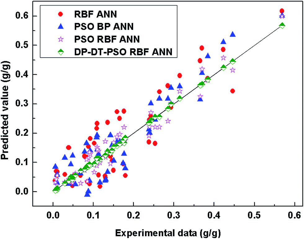 | ||
| Fig. 6 Predicted values vs. experimental data. | ||
The distribution of prediction data points shows significant differences among these models. The prediction data points of DP-DT-PSO RBF ANN model are the closest to the straight, indicating the high consistency with the experimental data. No abnormal prediction data point is found, indicating the better stability. The distance between the prediction data points and the straight line indicates that the accuracy of DP-DT-PSO RBF ANN model is also higher. Table 5 shows the data of the evaluation indexes for each model in the solubility prediction for various polymers.
| Model | PP | PLLA | HDPE | CPEs | PS | PBS | PBSA | PLGA | Average | |
|---|---|---|---|---|---|---|---|---|---|---|
| ARD | RBF ANN | 0.0098 | 0.0094 | 0.0088 | 0.0092 | 0.0093 | 0.0092 | 0.0091 | 0.0087 | 0.0092 |
| PSO BP ANN | 0.0052 | 0.0072 | 0.0082 | 0.0077 | 0.0056 | 0.0082 | 0.0089 | 0.0065 | 0.0072 | |
| PSO RBF ANN | 0.0046 | 0.0055 | 0.0054 | 0.0046 | 0.0054 | 0.0066 | 0.0061 | 0.0056 | 0.0055 | |
| This paper | 0.0025 | 0.0039 | 0.0048 | 0.0038 | 0.0039 | 0.0048 | 0.0039 | 0.0035 | 0.0039 | |
![[thin space (1/6-em)]](https://www.rsc.org/images/entities/char_2009.gif) |
||||||||||
| R2 | RBF ANN | 0.9643 | 0.9643 | 0.9651 | 0.9614 | 0.9612 | 0.9598 | 0.9601 | 0.9618 | 0.9623 |
| PSO BP ANN | 0.9813 | 0.9815 | 0.9816 | 0.9812 | 0.9821 | 0.9912 | 0.9811 | 0.9834 | 0.9829 | |
| PSO RBF ANN | 0.9885 | 0.9882 | 0.9863 | 0.9817 | 0.9811 | 0.9812 | 0.9817 | 0.9821 | 0.9839 | |
| This paper | 0.9962 | 0.9959 | 0.9961 | 0.9969 | 0.9957 | 0.9961 | 0.9957 | 0.9961 | 0.9961 | |
|
||||||||||
| RMSEP | RBF ANN | 0.0579 | 0.0615 | 0.0721 | 0.0852 | 0.0789 | 0.0566 | 0.0796 | 0.0886 | 0.0726 |
| PSO BP ANN | 0.0335 | 0.0345 | 0.0368 | 0.0369 | 0.0389 | 0.0411 | 0.0485 | 0.0512 | 0.0402 | |
| PSO RBF ANN | 0.0312 | 0.0352 | 0.0362 | 0.0338 | 0.0412 | 0.0431 | 0.0458 | 0.0437 | 0.0388 | |
| This paper | 0.0158 | 0.0134 | 0.0138 | 0.0161 | 0.0145 | 0.0156 | 0.0214 | 0.0134 | 0.0155 | |
Table 5 shows the prediction statistics of each model, including the data of accuracy and correlation. The model DP-DT-PSO RBF ANN has a better comprehensive performance including precision and correlation. Table 6 provides the average computation time required for 5 runs of each model.
| Model | Computation time (s) |
|---|---|
| RBF ANN | 36 |
| PSO BP ANN | 41 |
| PSO RBF ANN | 43 |
| This paper | 56 |
The computation time of RBF ANN model is the shortest. The computation time of DP-DT-PSO RBF ANN model is longer. Intelligent algorithm intervention is bound to consume more computation time. In addition, the diffusion theory is introduced into the DP-DT-PSO RBF ANN model for improving the algorithm. In each iteration, the thermodynamic parameters of the system will be recalculated. In addition, the intelligent algorithm itself belongs to the optimization method, and also requires the longer computation time. Its computation time is within the acceptable range.
4.3 Result analysis
In terms of efficiency, accuracy and correlation, the results show that the DP-DT-PSO RBF ANN model presents a good performances for solubility prediction with high accuracy and good correlations, the predicted data are agree with the experimental values. Fig. 7 depicts the corrections between predicted values and experimental data under the different temperatures and pressure.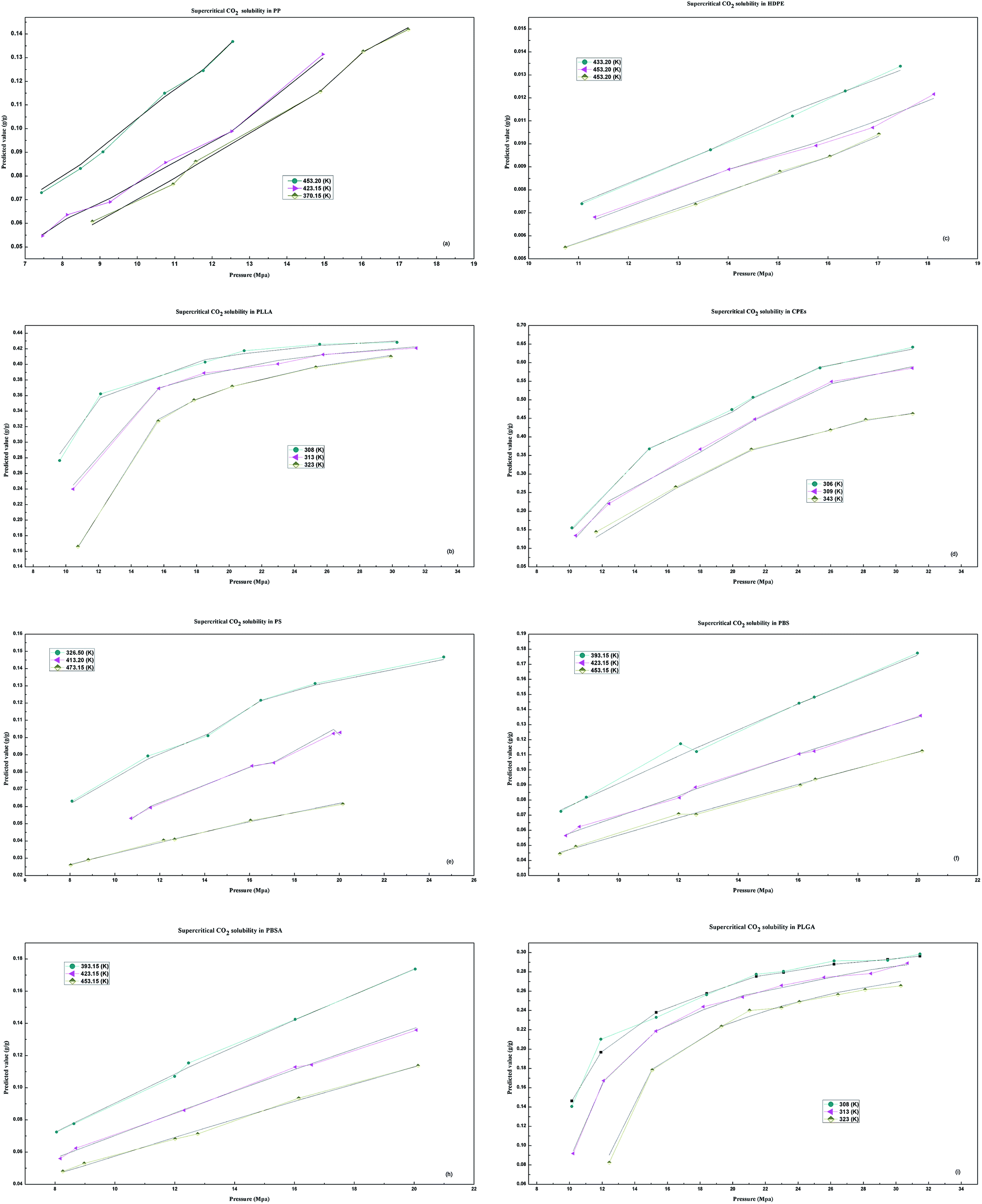 | ||
| Fig. 7 Variation of solubility with pressure and temperature. | ||
As we can see form Fig. 7, the solubility of HDPE, PS, PP, CPEs, PBS and PBSA is proportional to the pressure and inversely proportional to the temperature. As shown in Fig. 7(b) and (i), with the increase in the pressure, the solubility of the two polymers PLLA and PLGA increases firstly and then stabilizes and decreases with the increase in the temperature. The solubility prediction trend is concordant with the experimental.
5. Conclusions
(1) The prediction performance of DP-DT-PSO RBF ANN model is good.Based on the theory of diffusion, dissolution and particle evolution, an improved evolutionary algorithm based on diffusion theory is proposed in this paper to train the radial artificial neural network, so that the solution prediction model is obtained. A good prediction performance of DP-DT-PSO RBF ANN model is demonstrated by predicting the solubility examples of ScCO2 in 8 polymers.
(2) The expandability of DP-DT-PSO RBF ANN model is better.
By dissolubility prediction, this paper verifies the advantages of DP-DT-PSO RBF ANN model. The model can be extended to prediction fields of other chemical and physical properties. It can be applied to experimental data processing, control and optimization of experimental parameters. The scalability is better.
(3) DP-DT-PSO RBF ANN model realizes the solubility prediction by training experimental data and obtaining relevant rules. In the future research, the essence of diffusion and dissolution can be further discussed and the theoretical calculation method will be put forward. We will pay more attention to the development of this field and study the theoretical calculation method with the higher efficiency and better performance.
Conflicts of interest
There are no conflicts to declare.Abbreviations
| PVT | Pressure, volume, temperature |
| ANN | Artificial neural network |
| RBF | Radial basis function |
| PSO | Particle swarm optimization |
| DP-DT-PSO | Double population particle swarm algorithm based on diffusion theory |
| PBS | Poly(butylene succinate) |
| PBSA | Poly(butylene succinate-co-adipate) |
| PP | Polypropylene |
| PS | Polystyrene |
| CPEs | Carboxylated polyesters |
| PLLA | Poly(L-lactide) |
| PLGA | Poly(D,L-lactide-co-glycolide) |
| HDPE | High-density polyethylene |
| ARD | Average relative deviation |
| R2 | Squared correlation coefficient |
| MSE | Mean square error |
| RMSEP | Root mean square error of prediction |
Acknowledgements
The authors gratefully acknowledge the support from the National Natural Science Foundation of China (Grant Numbers: 51663001, 51463015).References
- A. A. Cockram, T. J. Neal, M. J. Derry, O. O. Mykhaylyk, N. S. J. Williams, M. W. Murray, S. N. Emmett and S. P. Armes, Macromolecules, 2017, 50, 796–802 CrossRef CAS PubMed.
- F. N. Azad, M. Ghaedi, A. Asfaram, A. Jamshidi, G. Hassani, A. Goudarzi, M. H. A. Azqhandi and A. Ghaedi, RSC Adv., 2016, 6, 19768–19779 RSC.
- M. T. Jacobsen, M. E. Petersen, X. Ye, M. Galibert, G. H. Lorimer, V. Aucagne and M. S. Kay, J. Am. Chem. Soc., 2016, 138, 11775–11782 CrossRef CAS PubMed.
- M. Li, W. Wu, B. Chen, Y. Wu and X. Huang, RSC Adv., 2017, 7, 35274–35282 RSC.
- H. Ziaee, S. M. Hosseini, A. Sharafpoor, M. Fazavi, M. M. Ghiasi and A. Bahadori, J. Taiwan Inst. Chem. Eng., 2015, 46, 205–213 CrossRef CAS.
- Y. S. Zhao, J. B. Gao, Y. Huang, R. M. Afzal, X. P. Zhang and S. J. Zhang, RSC Adv., 2016, 6, 70405–70413 RSC.
- J. J. van Franeker, G. H. L. Heintges, C. Schaefer, G. Portale, W. Li, M. M. Wienk, P. van der Schoot and R. A. J. Janssen, J. Am. Chem. Soc., 2015, 137, 11783–11794 CrossRef CAS PubMed.
- J. A. Lazzús, F. Cuturrufo, G. Pulgar-Villarroel, I. Salfate and P. Vega, Ind. Eng. Chem. Res., 2017, 56, 6869–6886 CrossRef.
- S. Arefi-Oskoui, A. Khataee and V. Vatanpour, ACS Comb. Sci., 2017, 19, 464–477 CrossRef CAS PubMed.
- J. R. Kramer and T. J. Deming, J. Am. Chem. Soc., 2014, 136, 5547–5550 CrossRef CAS PubMed.
- R. Galvelis and Y. Sugita, J. Chem. Theory Comput., 2017, 13, 2489–2500 CrossRef CAS PubMed.
- Y. Xu, D. Koo, E. A. Gerstein and C.-S. Kim, Polymer, 2016, 84, 121–131 CrossRef CAS.
- L. P. Barron and G. L. McEneff, Talanta, 2016, 147, 261–270 CrossRef CAS PubMed.
- H. T. Liu, Y. W. Wang, W. D. Huang and M. Lei, Environ. Sci. Pollut. Res., 2016, 23, 24230–24236 CrossRef CAS PubMed.
- X. Wang, W. Cai, J. Lu and Y. Sun, Ind. Eng. Chem. Res., 2014, 53, 19293–19303 CrossRef CAS.
- A. Esmaeili, E. Hejazi and Y. Vasseghian, RSC Adv., 2015, 5, 91776–91784 RSC.
- Y. Bakhbakhi, Math. Comput. Model., 2012, 55, 1932–1941 CrossRef.
- A. Z. Hezave, S. Raeissi and M. Lashkarbolooki, Ind. Eng. Chem. Res., 2012, 51, 9886–9893 CrossRef CAS.
- F. Gharagheizi, A. Eslamimanesh, A. H. Mohammadi and D. Richon, Ind. Eng. Chem. Res., 2011, 50, 221–226 CrossRef CAS.
- A. Eslamimanesh, F. Gharagheizi, A. H. Mohammadi and D. Richon, Chem. Eng. Sci., 2011, 66, 3039–3044 CrossRef CAS.
- H. Pahlavanzadeh, S. Nourani and M. Saber, J. Chem. Thermodyn., 2011, 43, 1775–1783 CrossRef CAS.
- D. Granato, M. D. Carrapeiro, V. Fogliano and S. M. van Ruth, Trends Food Sci. Technol., 2016, 52, 31–48 CrossRef CAS.
- A. S. Ghareb, A. Abu Bakar and A. R. Hamdan, Expert Syst. Appl., 2016, 49, 31–47 CrossRef.
- R. Xia, X. Huang and M. Li, J. Appl. Polym. Sci., 2016, 133, 44252 Search PubMed.
- M. Tang, C.-E. Hu, Z.-L. Lv, X.-R. Chen and L.-C. Cai, J. Phys. Chem. A, 2016, 120, 9489–9499 CrossRef CAS PubMed.
- C.-P. Chou, Y. Nishimura, C.-C. Fan, G. Mazur, S. Irle and H. A. Witek, J. Chem. Theory Comput., 2016, 12, 53–64 CrossRef CAS PubMed.
- M. Saidi-Mehrabad, S. Dehnavi-Arani, F. Evazabadian and V. Mahmoodian, Comput. Ind. Eng., 2015, 86, 2–13 CrossRef.
- X. G. Liu and C. Y. Zhao, AIChE J., 2012, 58, 1194–1202 CrossRef CAS.
- J. A. Lazzus, A. Ponce and L. Chilla, Fluid Phase Equilib., 2012, 317, 132–139 CrossRef CAS.
- A. Khajeh and H. Modarress, Expert Syst. Appl., 2010, 37, 3070–3074 CrossRef.
- M. A. Hussain, M. K. Aroua, C. Y. Yin, R. A. Rahman and N. A. Ramli, Korean J. Chem. Eng., 2010, 27, 1864–1867 CrossRef CAS.
- M. S. Li, X. Y. Huang, H. S. Liu, B. X. Liu and Y. Wu, J. Appl. Polym. Sci., 2013, 130, 3825–3832 CrossRef CAS.
- M. S. Li, X. Y. Huang, H. S. Liu, B. X. Liu, Y. Wu and F. R. Ai, Acta Chimica Sinica, 2013, 71, 1053–1058 CrossRef CAS.
- Y. Wu, B. X. Liu, M. S. Li, K. Z. Tang and Y. B. Wu, Chin. J. Chem., 2013, 31, 1564–1572 CrossRef CAS.
- M. S. Li, X. Y. Huang, H. S. Liu, B. X. Liu, Y. Wu and X. Z. Deng, J. Appl. Polym. Sci., 2013, 129, 3297–3303 CrossRef CAS.
- M. Li, X. Huang, H. Liu, B. Liu, Y. Wu and L. Wang, RSC Adv., 2015, 5, 45520–45527 RSC.
- M. S. Li, X. Y. Huang, H. S. Liu, B. X. Liu, Y. Wu, A. H. Xiong and T. W. Dong, Fluid Phase Equilib., 2013, 356, 11–17 CrossRef CAS.
- X. Ru-Ting and H. Xing-Yuan, RSC Adv., 2015, 5, 76979–76986 RSC.
- J. Kennedy and R. Eberhart, Particle swarm optimization, Perth, Aust, 1995, DOI:10.1109/icnn.1995.488968.
- X. L. Zhao, M. Turk, W. Li, K. C. Lien and G. Z. Wang, Applied Soft Computing, 2016, 48, 151–159 CrossRef.
- A. Khajeh, H. Modarress and M. Mohsen-Nia, Iran. Polym. J., 2007, 16, 759–768 CAS.
- Y. Sato, K. Fujiwara, T. Takikawa, Sumarno, S. Takishima and H. Masuoka, Fluid Phase Equilib., 1999, 162, 261–276 CrossRef CAS.
- Z. G. Lei, H. Ohyabu, Y. Sato, H. Inomata and R. L. Smith, J. Supercrit. Fluids, 2007, 40, 452–461 CrossRef CAS.
- D. C. Li, T. Liu, L. Zhao and W. K. Yuan, Ind. Eng. Chem. Res., 2009, 48, 7117–7124 CrossRef CAS.
- E. Aionicesei, M. Skerget and Z. Knez, J. Supercrit. Fluids, 2008, 47, 296–301 CrossRef CAS.
- M. Skerget, Z. Mandzuka, E. Aionicesei, Z. Knez, R. Jese, B. Znoj and P. Venturini, J. Supercrit. Fluids, 2010, 51, 306–311 CrossRef CAS.
- Y. Sato, M. Yurugi, K. Fujiwara, S. Takishima and H. Masuoka, Fluid Phase Equilib., 1996, 125, 129–138 CrossRef CAS.
- S. Hilic, S. Boyer, A. Padua and J. Grolier, J. Polym. Sci., Part B: Polym. Phys., 2001, 39, 2063–2070 CrossRef CAS.
- Y. Sato, T. Takikawa, S. Takishima and H. Masuoka, J. Supercrit. Fluids, 2001, 19, 187–198 CrossRef CAS.
- Y. Sato, T. Takikawa, A. Sorakubo, S. Takishima, H. Masuoka and M. Imaizumi, Ind. Eng. Chem. Res., 2000, 39, 4813–4819 CrossRef CAS.
| This journal is © The Royal Society of Chemistry 2017 |