
 Open Access Article
 This Open Access Article is licensed under a Creative Commons Attribution-Non Commercial 3.0 Unported Licence
In silico prediction of chronic toxicity with chemical category approaches†
Xiao Li‡
 *ab,
Yuan Zhang‡b,
Hongna Chenc,
Huanhuan Lib and
Yong Zhao*ab
*ab,
Yuan Zhang‡b,
Hongna Chenc,
Huanhuan Lib and
Yong Zhao*ab
aBeijing Computing Center, Beijing Academy of Science and Technology, 7 Fengxian Road, Beijing 100094, China. E-mail: zhaoyong@bcc.ac.cn; lixiao@bcc.ac.cn; lixiao1688@163.com; Fax: +86-10-5934-1855; Tel: +86-10-5934-1764 Tel: +86-10-5934-1890
bBeijing Beike Deyuan Bio-Pharm Technology Co.Ltd., 7 Fengxian Road, Beijing 100094, China
cTigermed Consulting Co., Ltd., 20 Chaowai Street, Beijing 100020, China
First published on 23rd August 2017
Abstract
Chemical chronic toxicity, referring to the toxic effect of a chemical following long-term or repeated sub lethal exposures, is an important toxicological end point in drug design and environmental risk assessment. Owing to the high cost and laboriousness in experimental tests, it is very necessary to develop in silico methods to assess the chronic toxicity of compounds. In this paper, we collected a large data set containing 567 diverse compounds with the lowest observed adverse effect level (LOAEL) values determined in rats by oral administration. A series of models were developed combining with five machine learning methods and six fingerprint types based on four different thresholds discriminated chemicals with chronic toxicity from those without chronic toxicity. Meanwhile, chemicals were also grouped into three classes (strong, moderate and weak chronic toxicity) and models were developed using the extreme parts (strong and weak chronic toxicity). Finally, we proposed eight privileged substructures using substructure frequency analysis method. These privileged substructures could be regarded as structural alerts of chronic toxicity. The models and privileged substructures could provide critical information and useful tools for chemical chronic toxicity assessment in drug discovery and environmental risk assessment.
Introduction
Chronic toxicity refers to the general toxicological effects in animals occurring as a result of repeated exposure (oral, dermal or inhalation) to a substance over a specific period of time.1 It is one of the toxicological endpoints posing the highest concern of people. Generally, chronic toxicity is often assessed in rodents with various doses of test chemicals over a long period of time (unusually more than 180 days).2 The chronic studies are used to establish a dose metric for risk assessment, the lowest observed adverse effect level (LOAEL) or no observed adverse effect level (NOAEL). LOAEL is the lowest dose that induces an adverse effect and NOAEL indicates the dose at which no effects are observed.3 For NOAEL and LOAEL, the measurement unit is expressed as mg per kg per day.Chemicals in drugs and consumer goods are an integral part of our everyday life, and we are exposed to these chemicals over longer periods of time. Therefore, it is quite important to evaluate the chronic toxicity of chemicals in consumer goods and pharmaceutical compounds. The accurate determination of chemical chronic toxicity should be performed by long-term animal studies. However, this approach is very expensive and time consuming; especially, it is not appropriate for screening of large-batch compounds or virtual molecules. Thus, the application of in silico approaches could provide an alternative means of estimating chemical chronic toxicity.
Since chronic toxicity is not really a single endpoint, the mechanisms of a multitude of biological effects are quite diverse. It is a great challenge for accurate prediction of chronic toxicity nowadays. In the past decades, there have been only a few attempts to develop QSAR models for chronic toxicity in mammalian. In 2005, de Julian-Ortiz et al.4 used a dataset of 234 compounds with LOAEL data compiled from different sources to model chronic toxicity by multilinear regression (MLR) and linear discriminant analysis (LDA). Variable selection was performed by means of the Furnival–Wilson algorithm in MLR. In addition, a subset contained 86 compounds extracted from U.S. EPA documents was also assessed by MLR analysis. The performance on the homogeneous subset was significantly better (coefficient of determination (R2) was 0.647 and root mean square error (RMSE) was 0.66) than that on the structurally heterogeneous dataset (R2 = 0.524 and RMSE = 0.74). Unfortunately, the models were not validated with external set. Subsequently, García-Domenech et al.5 built another regression model using MLR method along with the same EPA subset used by De Julián-Ortiz et al. The model was validated on 16 external chemicals. R2 values in the training set and external validation set were 0.795 and 0.712, respectively. García-Domenech's model showed good performances both on internal and external validation. However, the generalizability of the model was restricted due to the lack of structural diversity. Mazzatorta et al.2 reported an excellent study on the in silico prediction of LOAEL based on two-dimensional chemical descriptors and multivariate analysis. They constructed a data set of 567 entries referring to 445 different chemicals with LOAEL data (180 days or more of oral exposure in rats) selected from several sources. Then, an integrated approach of genetic algorithm (GA) and partial least squares (PLS) was applied to select variables. Finally, leave-one-out stepwise multiple linear regression (LOO-SMLR) was used to generate the predictive model. The RMSE of the predictive model is 0.73 (in a logarithmic scale) on the leave-one-out (LOO) cross validation and is close to the estimated variability of experimental values (0.64). One of the most recent models for the prediction of LOAEL was reported by Gadaleta et al.6 They employed a customized k-nearest neighbors (k-NN) approach for predicting sub-chronic oral toxicity (from 84 to 98 days) in rats. A training set of 254 chemicals was used to derive models and the predictive power of models was evaluated on an external dataset comprising 179 chemicals. The models give good results with R2 ≥ 0.543 on external validation.
The primary goal of toxicity prediction is to distinguish between toxicologically active and inactive compounds. The classification model can also play an important role in risk assessment. However, there have been few reports on the classification models for chronic toxicity prediction, although it is difficult for regression models to achieve the desired predictive power. In this study, we focused on the development of classification models and the identification of structural alerts for oral rat chronic toxicity. Since there is lack of specific thresholds to discriminate chemicals with chronic toxicity from those without chronic toxicity, we tested four LOAEL values as thresholds to find the most suitable threshold for definition of toxicity category. On the basis of a large and open source data set, we proposed a series of binary models using different molecular fingerprints along with different machine learning algorithms. Furthermore, substructure frequency analysis method based on SubFP fingerprints was employed for the identification of privileged substructures responsible for chemical chronic toxicity.
Materials and methods
Data preparation
In this study, all the data were collected from two sources, totally containing 576 chemicals with oral rat chronic toxicity in LOAEL values.The first data set was obtained from Mazzatorta's work.2 The data set was carefully prepared in the following steps: (1) removing mixtures, inorganic and organometallic compounds; (2) salts were converted to their corresponding acidic or basic forms, and water molecules were removed from the hydrates; (3) removing compounds with molecular weights less than 40 or more than 800; (4) only one stereoisomer was retained because the 2D fingerprints of a pair of stereoisomers are identical; (5) for the chemicals with two or more entries, the averaged LOAEL values were used after removing duplicated molecules. The final data set contained 431 compounds with measured LOAEL values.
To further evaluate the predictive ability of the models, compounds with oral rat chronic toxicity were extracted from the U.S. EPA's Toxicity Reference Database (ToxRefDB)7 and used as an external validation set. After removal of duplicates, the external validation set contained 145 compounds. All data sets were given in Table S1 of the ESI.†
Since there is a lack of specific threshold for discriminating chemicals with chronic toxicity from those without chronic toxicity, we tested four LOAEL values (5 mg per kg per day, 10 mg per kg per day, 50 mg per kg per day and 100 mg per kg per day) as thresholds to find the most suitable threshold for our data set. Moreover, the chemicals with LOAEL ≤ 10 mg per kg per day were labeled as strong chronic toxicity, chemicals with LOAEL > 50 mg per kg per day were labeled as weak chronic toxicity and chemicals with LOAEL ranged from 10 to 50 mg per kg per day were labeled as medium chronic toxicity.
Calculation of molecular fingerprints
Molecular fingerprints have been widely used in similarity searching and classification modeling,8–12 since fingerprints were generated directly from chemical structures, and could be easily translated into two-dimensional fragments. Each molecule was described as a binary string of structural keys. The predefined dictionary contained a SMARTS list of substructure patterns. For a SMARTS pattern, if a specified substructure is presented in the given molecule, the corresponding bit is set to “1”; conversely, it is set to “0”. In the present work, six types of fingerprints were used, including the CDK fingerprint (FP, 1024 bits), CDK extended fingerprint (extended, 1024 bits), estate fingerprint (estate, 79 bits), MACCS keys (MACCS, 166 bits), PubChem fingerprint (PubChem, 881 bits) and substructure fingerprint (SubFP, 307 bits). All the fingerprints were calculated by the PaDEL Descriptor software.13Model building
Five machine learning methods were employed for model building, including support vector machine (SVM), k-nearest neighbor (kNN), C4.5 decision tree (C4.5),random forest (RF) and naive Bayes (NB) algorithms. SVM algorithm was implemented in the open source LIBSVM (LIBSVM 3.16 package),14 and the other four algorithms were performed in Orange 2.6 (version 2.6.1, freely available at http://www.ailab.si/orange/).15In the present work, the parameters of C4.5 DT, RF and NB algorisms were default in Orange toolbox.
Assessment of model performance
All models were validated by 5-fold cross validation and a diverse external validation set. The performances of models were assessed by several statistical parameters. The sensitivity (SE) and specificity (SP) are two measures applicable to binary classifications, which denote the ratios of positive instances and negative instances correctly identified, respectively. The accuracy (Q) is the total correct predictive accuracy of samples, and the Matthews correlation coefficient (MCC) is generally regarded as a balanced measure which can be used even if the classes are of very different sizes. MCC returns a value between −1 and 1. A coefficient of 1 represents a perfect prediction, 0 means no better than random prediction and −1 indicates total disagreement between prediction and observation. These parameters can be calculated with eqn (1)–(4).
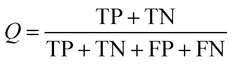 | (1) |
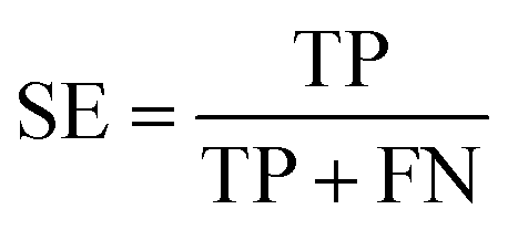 | (2) |
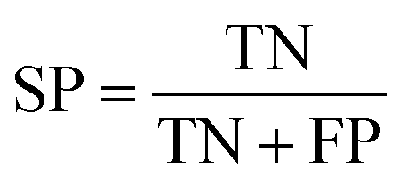 | (3) |
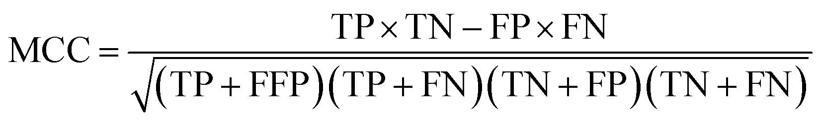 | (4) |
In these equations, TP, TN, FP, FN are the numbers of true positives, true negatives, false positives and false negatives, respectively.
In addition, the AUC value, which means the area under the receiver operating characteristic (ROC) curve, was also computed to estimate the predictive accuracy of the models. The AUC value is the probability of positive compounds being ranked earlier than decoy compounds, it ranges from 0.5 (useless random classifiers) to 1 (perfect classifiers).
Identification of structural alerts or privileged substructures
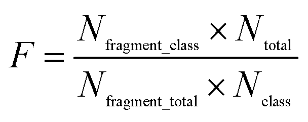
Structural alerts (SAs) or privileged substructures are defined as molecular functional groups that can cause toxicity, and their presence alerts investigators to the potential toxicities of test chemicals.23,24 SAs are important predictive tools for toxicity. They can be derived directly from mechanistic knowledge.25In this study, we analyzed the privileged substructure fragments using substructure frequency analysis26 methods based on SubFP. If a substructure was more frequently presented in chemicals with strong chronic toxicity (LOAEL ≤ 10 mg per kg per day) than those with weak chronic toxicity (LOAEL > 50 mg per kg per day), this substructure was called a privileged substructure involved in chemical chronic toxicity. The “frequency of a fragment” enrichment factor in chemicals was defined as follows:
 | (5) |
Results and discussion
Data analysis
For purpose of ensuring the data homogeneity, our analysis was restricted to chronic (defined as longer than 180 days), rat and oral studies. After careful data preparation, a large diverse and high quality of chronic toxicity database was constructed, which contained 576 unique chemicals with oral rat chronic toxicity in LOAEL values. The training set and external validation set contained 431 and 145 compounds, separately. The statistics of the training and external validation sets were summarized in Table 1.| Data sets | Thresholds (mg per kg per day) | |||||
|---|---|---|---|---|---|---|
| (0, 5) | (5, 10) | (10, 50) | (50, 100) | (100, ∞) | Total | |
| Training set | 94 | 39 | 133 | 39 | 126 | 431 |
| External validation set | 36 | 13 | 44 | 21 | 31 | 145 |
| Total | 130 | 52 | 177 | 60 | 157 | 576 |
As we known, the diversity of data set is a key issue for global model development. QSAR models based on relatively small dataset or homologous compounds always resulted in poor generalization abilities. In this study, the radar chart analysis was performed to explore the chemical space of the entire data set. As shown in Fig. 1, the A![[thin space (1/6-em)]](https://www.rsc.org/images/entities/char_2009.gif) logP ranged from −4.22 to 10.45, molecular solubility ranged from −12.00 to 0.97, molecular weights ranged from 42.04 to 745.98, the number of H-acceptors ranged from 0 to 14, and the number of H-donors ranged from 0 to 7. These data indicated that the 576 compounds used in our data set covered a sufficient large chemical space.27
logP ranged from −4.22 to 10.45, molecular solubility ranged from −12.00 to 0.97, molecular weights ranged from 42.04 to 745.98, the number of H-acceptors ranged from 0 to 14, and the number of H-donors ranged from 0 to 7. These data indicated that the 576 compounds used in our data set covered a sufficient large chemical space.27
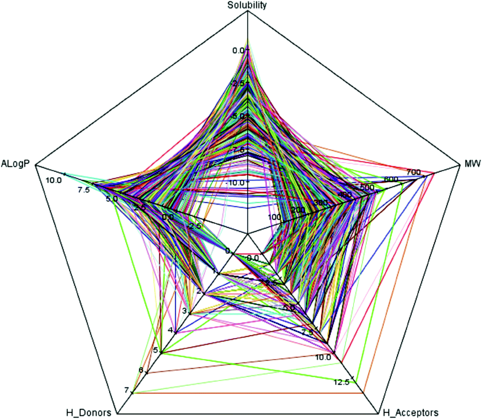 | ||
| Fig. 1 The radar chart of five simple descriptors: molecular solubility (solubility), AlogP, molecular weight (MW), the number of hydrogen bond acceptors (H-acceptors) and the number of hydrogen bond donors (H-donors) for the entire data set of 576 compounds were presented. Each color line represents a compound. | ||
In order to further explore the chemical diversity of our data set, the Tanimoto similarity index28 was also calculated with ECFC-4 fingerprint, which has been widely used to evaluate similarities among chemicals. The entire data set was separated into 100 clusters, and the heat map of Tanimoto similarity index of the cluster center molecules was plotted in Fig. 2. The average Tanimoto similarity index was 0.191, indicating that the chemicals in our data set were evidently diverse.
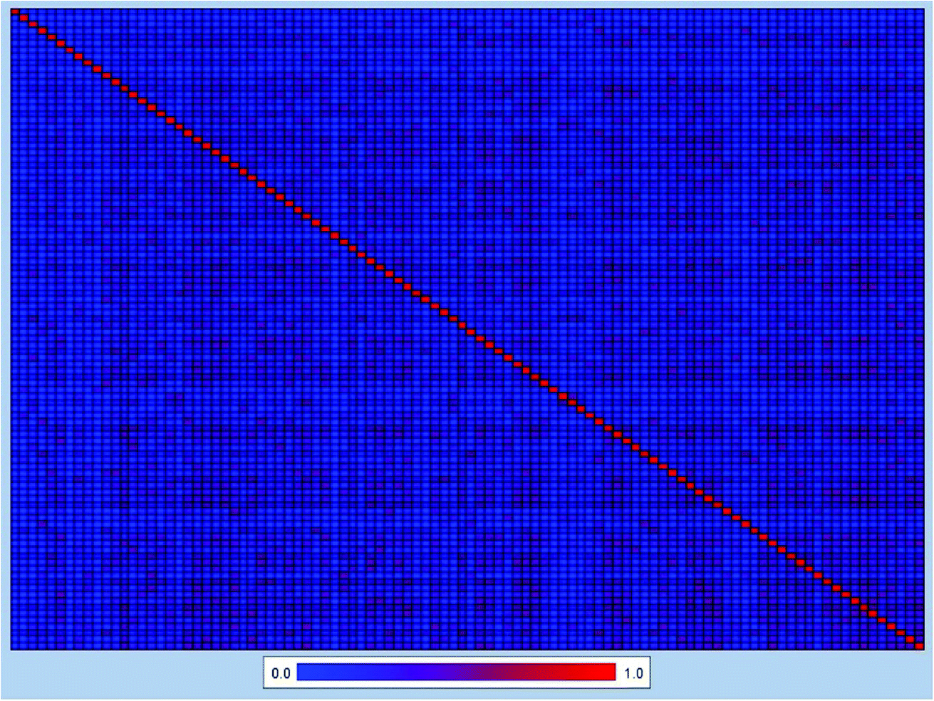 | ||
| Fig. 2 Heat map of molecular similarity plotted by the Tanimoto similarity index using ECFC-4 fingerprint of 100 cluster center molecules. The average Tanimoto similarity index was 0.191. x-axis and y-axis represented the number of 100 cluster center molecules, respectively. | ||
Performance of different models
Based on four different LOAEL threshold values, the binary classification models were built using five machine learning algorithms along with six fingerprint types. As a result, there were a total of 120 models generated by combination (30 models for each threshold). When developed the models, the parameters of C4.5 DT, RF and NB algorisms were default in Orange toolbox. For kNN algorism, the parameter of k = 5 was used and the nearness was measured by Euclidean distance metrics. The SVM parameters C and γ for all models were selected with grid search method and shown in Table S2.†The 5-fold cross validation technique was used to evaluate the model robustness, and performances of the models were shown in Table S3 of the ESI.† We can found that the models at 5 mg per kg per day threshold performed better than the others. Three algorisms namely SVM, Random Forest and kNN yielded the best predictive performances. The model developed by Random Forest algorism along with SubFP fingerprint at 5 mg per kg per day threshold had the best predictive ability for 5-fold cross validation and yielded overall accuracy of 84.2%.
External validation of models
An external validation set independent of the training set was used to further evaluate the robustness and prediction ability of the models. As the external validation set was not used to develop the models, the performances on external validation could objectively reflect the predictive capability of the models. The performances of models on external validation can be seen in Table S4.† It is easy to see that the values of overall accuracy among the models at threshold with 5 mg per kg per day, 10 mg per kg per day, 50 mg per kg per day and 100 mg per kg per day range from 72.4% to 86.2%, 61.4–77.2%, 49.7–71.0% and 52.4–69.0%, respectively. Similar to the 5-fold cross validation results, the models at 5 mg per kg per day threshold also performed best on external validation, especially, the kNN model based on estate fingerprint yielded the accuracy of 86.21%.Models with strong and weak chronic toxicity (LOAEL ≤ 10 mg per kg per day or LOAEL > 50 mg per kg per day)
As mentioned before, the chemicals in our data set were also grouped into three classes: strong chronic toxicity (chemicals with LOAEL ≤ 10 mg per kg per day), weak chronic toxicity (chemicals with LOAEL > 50 mg per kg per day) and medium chronic toxicity (chemicals with LOAEL from 10 to 50 mg per kg per day). In the studies of QSAR modeling, people always considered all available information by using all of the compounds for model building. However, the predictive power of models is often affected by the error range of the experimental results. To avoid this problem, Roche, et al.29 proposed the “likeness concept”, which only uses the extremes of the data set (strong and weak chronic toxicity classes in this study). This concept has been used in many studies in the past years.30–33 In the present study, we also developed a series of models followed this concept. The training set contained 133 chemicals with strong chronic toxicity (LOAEL ≤ 10 mg per kg per day) and 165 chemicals with weak chronic toxicity (LOAEL > 50 mg per kg per day), meanwhile the validation set contained 49 chemicals with strong chronic toxicity and 51 chemicals with weak chronic toxicity.A total of 30 classification models were also developed by combination of five machine learning methods and six fingerprint types. The performances of models for the 5-fold cross validation and external validation were shown in Table 2. We can find that the model built with SVM algorithm and MACCS keys gave the best result on 5-fold validation with prediction accuracy 76.9%, SE 70.7%, SP 81.8%, and MCC close to 0.529. For external validation, the MACCS-SVM model also achieved high prediction accuracy at 75.0%, and the values of sensitivity, specificity and MCC were 73.5%, 76.5% and 0.500, respectively. Another model, FP-SVM, gave good results on the validation set with prediction accuracy 75.0% and MCC close to 0.500, too.
| Model | 5-Fold validation on training set | External validation | ||||||||
|---|---|---|---|---|---|---|---|---|---|---|
| Q | SE | SP | AUC | MCC | Q | SE | SP | AUC | MCC | |
| Estate_kNN | 0.708 | 0.632 | 0.770 | 0.773 | 0.406 | 0.730 | 0.714 | 0.745 | 0.814 | 0.460 |
| Estate_SVM | 0.732 | 0.647 | 0.800 | 0.783 | 0.453 | 0.710 | 0.674 | 0.745 | 0.788 | 0.420 |
| Estate_RF | 0.691 | 0.451 | 0.885 | 0.789 | 0.378 | 0.630 | 0.347 | 0.902 | 0.761 | 0.300 |
| Estate_NB | 0.728 | 0.617 | 0.818 | 0.751 | 0.446 | 0.650 | 0.633 | 0.667 | 0.730 | 0.300 |
| Estate_DT | 0.715 | 0.707 | 0.721 | 0.722 | 0.426 | 0.640 | 0.674 | 0.608 | 0.724 | 0.282 |
| Extend_kNN | 0.722 | 0.594 | 0.824 | 0.765 | 0.433 | 0.700 | 0.612 | 0.784 | 0.799 | 0.403 |
| Extend_SVM | 0.738 | 0.677 | 0.788 | 0.792 | 0.468 | 0.720 | 0.674 | 0.765 | 0.808 | 0.440 |
| Extend_RF | 0.638 | 0.481 | 0.764 | 0.750 | 0.256 | 0.710 | 0.633 | 0.784 | 0.717 | 0.422 |
| Extend_NB | 0.691 | 0.677 | 0.703 | 0.742 | 0.378 | 0.610 | 0.612 | 0.608 | 0.691 | 0.220 |
| Extend_DT | 0.678 | 0.647 | 0.703 | 0.650 | 0.349 | 0.700 | 0.694 | 0.706 | 0.690 | 0.400 |
| FP_kNN | 0.732 | 0.594 | 0.842 | 0.772 | 0.454 | 0.720 | 0.612 | 0.824 | 0.769 | 0.447 |
| FP_SVM | 0.728 | 0.647 | 0.794 | 0.797 | 0.447 | 0.750 | 0.755 | 0.745 | 0.818 | 0.500 |
| FP_RF | 0.637 | 0.436 | 0.800 | 0.743 | 0.255 | 0.650 | 0.531 | 0.765 | 0.799 | 0.304 |
| FP_NB | 0.694 | 0.647 | 0.733 | 0.725 | 0.381 | 0.650 | 0.714 | 0.588 | 0.698 | 0.305 |
| FP_DT | 0.611 | 0.564 | 0.649 | 0.599 | 0.212 | 0.690 | 0.714 | 0.667 | 0.706 | 0.381 |
| MACCS_kNN | 0.735 | 0.722 | 0.746 | 0.811 | 0.466 | 0.730 | 0.776 | 0.686 | 0.817 | 0.463 |
| MACCS_SVM | 0.769 | 0.707 | 0.818 | 0.822 | 0.529 | 0.750 | 0.735 | 0.765 | 0.823 | 0.500 |
| MACCS_RF | 0.695 | 0.571 | 0.794 | 0.815 | 0.376 | 0.710 | 0.633 | 0.784 | 0.768 | 0.422 |
| MACCS_NB | 0.728 | 0.692 | 0.758 | 0.782 | 0.450 | 0.670 | 0.735 | 0.608 | 0.719 | 0.345 |
| MACCS_DT | 0.655 | 0.624 | 0.679 | 0.633 | 0.302 | 0.670 | 0.755 | 0.588 | 0.695 | 0.348 |
| Pubchem_kNN | 0.718 | 0.654 | 0.770 | 0.764 | 0.427 | 0.740 | 0.796 | 0.686 | 0.832 | 0.485 |
| Pubchem_SVM | 0.708 | 0.647 | 0.758 | 0.786 | 0.407 | 0.700 | 0.776 | 0.628 | 0.767 | 0.407 |
| Pubchem_RF | 0.705 | 0.556 | 0.824 | 0.791 | 0.398 | 0.650 | 0.531 | 0.765 | 0.718 | 0.304 |
| Pubchem_NB | 0.691 | 0.654 | 0.721 | 0.728 | 0.375 | 0.600 | 0.714 | 0.490 | 0.590 | 0.210 |
| Pubchem_DT | 0.701 | 0.669 | 0.727 | 0.701 | 0.396 | 0.640 | 0.755 | 0.529 | 0.674 | 0.292 |
| SubFP_kNN | 0.705 | 0.677 | 0.727 | 0.775 | 0.403 | 0.700 | 0.714 | 0.686 | 0.736 | 0.401 |
| SubFP_SVM | 0.728 | 0.647 | 0.794 | 0.818 | 0.447 | 0.660 | 0.674 | 0.647 | 0.764 | 0.321 |
| SubFP_RF | 0.708 | 0.444 | 0.921 | 0.823 | 0.424 | 0.610 | 0.306 | 0.902 | 0.742 | 0.260 |
| SubFP_NB | 0.701 | 0.669 | 0.727 | 0.716 | 0.396 | 0.640 | 0.714 | 0.569 | 0.669 | 0.286 |
| SubFP_DT | 0.701 | 0.684 | 0.715 | 0.698 | 0.398 | 0.670 | 0.633 | 0.706 | 0.667 | 0.340 |
Effects of machine learning algorisms and fingerprints used in model building
We used five machine learning methods for model building in this study. The results indicated that the models built with kNN and SVM algorisms performed much better both on 5-fold validation and external validation. These two machine learning methods are easier to use than the others and the parameters in the model are easy to organize. SVM has been well known as a powerful tool for the nonlinear problems, especially for binary classification. It can provide a good out-of-sample generalization with the appropriately selected parameters. kNN can give good results in model building should be attributed to its special algorithm and the structural characterization methods used in this study. The toxicity of compounds are always caused by some structural features, which can be represented by the molecular fingerprints. The same category must have some fingerprint similarity, thus a compound can be classified in accordance with the majority of its nearest neighbors.From the performance of models, we can find that the models used MACCS fingerprints as attributes were always better than the others. MACCS fingerprints package is based on the well-defined structural fragments dictionary. It contains much structural information. This result is in agreement with several previously published work that the MACCS keys is a good structural characterization method for chemical toxicity prediction.8–12
Relevance of thresholds to chronic toxicity
There is a lack of definite threshold for discrimination of chemicals with chronic toxicity from those without chronic toxicity, which made it a great challenge for chronic toxicity prediction. Herein, we selected four LOAEL values (5, 10, 50 and 100 mg per kg per day) as thresholds for model building. The results revealed that models built with threshold 5 mg per kg per day achieved the best performance. The models at threshold 5 mg per kg per day have high predictive accuracies both on 5-fold validation (from 71.0% to 84.2%) and external validation (from 72.4% to 86.2%). However, the predictive ability of these models were still unsatisfactory because of the low SE (from 21.3% to 55.3% for 5-fold validation and 19.4–66.7% for external validation) values resulted from the huge imbalance between positive and negative compounds (94 and 337). Besides, molecules with similar features were often classified into different classes based on individual thresholds. This kind of situation should always affect the predictive power of the models.To avoid this problem, we also grouped the chemicals in our data set into three classes (strong chronic toxicity, moderate chronic toxicity and weak chronic toxicity) and developed models using the extreme parts (strong and weak chronic toxicity). Compared with the models built at threshold 5 mg per kg per day, the SE values of models using the extreme parts were significantly improved and more balanced with SP values, although the overall prediction accuracies were slightly lower. In fact, it is very difficult to develop QSAR models for chronic toxicity with prediction accuracies as high as the single toxic endpoints with specific mechanism(s). Because the mechanisms of action of general toxicity are quite complex and diverse, which always involved with a wide range of possible adverse effects.
Analysis of structural alerts
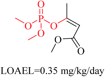
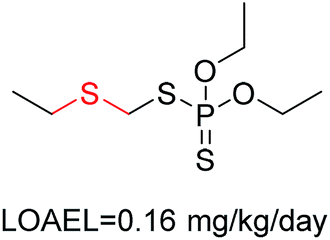
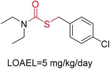
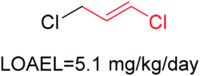
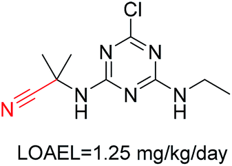
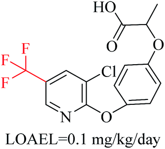
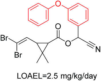
Structural alerts have been well defined and widely used in chemical carcinogenicity research. In the present study, substructure frequency analysis was employed to analyze the privileged substructures of chronic toxicity in SubFP fingerprints. Only the fragments presented in 10 or more molecules were analyzed. From the results of analysis of frequency, eight privileged substructures (phosphoric acid derivative, phosphoric triester, sulfenic derivative, carbodithioic ester, chloroalkene, nitrile, trifluoromethyl and diarylether) presented more frequently in chemicals with strong chronic toxicity. It meant that these substructures should be responsible for the chemical chronic toxicity. These privileged fragments were shown in Table 3.| No. | Description | SMARTS | Fragment frequency | General structure | Representative compound | |
|---|---|---|---|---|---|---|
| Positive | Negative | |||||
| 1 | Phosphoric acid derivative | [PX4D4](![[double bond, length as m-dash]](https://www.rsc.org/images/entities/char_e001.gif) [!#6])([!#6])([!#6])[!#6] [!#6])([!#6])([!#6])[!#6] |
2.096 | 0.077 | 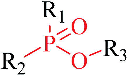 |
 |
| 2 | Phosphoric triester | [PX4D4]([OX1])([OX2][#6; !$(C[O,N,S])])([OX2][#6; !$(C[O,N,S])])[OX2][#6; !$(C[O,N,S])] |
1.968 | 0.184 | 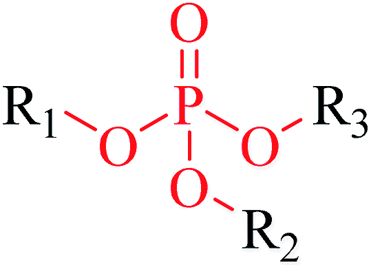 |
 |
| 3 | Sulfenic derivative | [SX2; $([H1]),$([H0][#6])][!#6] | 1.913 | 0.230 |  |
 |
| 4 | Carbodithioic ester | [CX3; !R; $([C][#6]),$([CH]); $([C]([SX1])[SX2][#6; !$(C[O,N,S])])] |
1.670 | 0.436 | 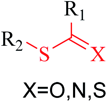 |
 |
| 5 | Chloroalkene | [ClX1][CX3][CX3] |
1.662 | 0.442 | 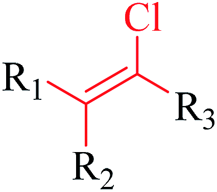 |
 |
| 6 | Nitrile | [NX1]#[CX2] | 1.598 | 0.496 |  |
 |
| 7 | Trifluoromethyl | FX1[CX4; !$([H0][Cl,Br,I]); !$([F][C]([F])([F])[F])](FX1)(FX1) | 1.584 | 0.508 | 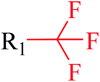 |
 |
| 8 | Diarylether | [c][OX2][c] | 1.458 | 0.614 |  |
 |
Phosphonic acid derivative and phosphoric trimester were phosphorus fragments, which exist in a large class of pesticides as organophosphates. Chemicals contained these two fragments can inhibit the activity of cholinesterase and result in the accumulation of acetylcholine, which is a neurotransmitter of the cholinergic receptor. They can also take direct effect on the cholinergic receptor, which can lead the next neuron or effector to excessive excitement or inhibition.8,34 The chronic toxicity of chemicals contained nitrile mainly due to the release of cyanide anions through hydrolysis.8,35 The fragments phosphoric acid derivative, phosphoric triester, sulfenic derivative, chloroalkene and nitrile were also identified as structural alerts responsible for acute toxicity.8 As structural constituents, diaryl ether group is also common in numerous pesticides, such as nitrodiphenyl ethers, pyrethroids, pyrimidinyloxybenzoates, and so on. We believe these meaningful substructures can potentially provide scaffolds and be interpreted by chemists to gain understanding and guide modification information to reduce chemical chronic toxicity.
Conclusions
In this study, we focused on the in silico prediction of chemical chronic toxicity. A large diverse data set contained 567 unique compounds with rat oral chronic toxicity data was used for model building. Since there is a lack of definite threshold for discrimination of chemicals with chronic toxicity from those without chronic toxicity, we selected four LOAEL values (5, 10, 50 and 100 mg per kg per day) as thresholds for model building. A series of binary classification models were developed using five machine learning methods along with six fingerprint types. All the models were validated on 5-fold validation and external validation. The models at threshold 5 mg per kg per day performed better than others, but the predictive ability of these models were still unsatisfactory because of the low SE values. As molecules with similar features are often classified into different classes based on individual thresholds, we also grouped the chemicals into three classes (strong chronic toxicity, moderate chronic toxicity and weak chronic toxicity) and developed models using the extreme parts (strong and weak chronic toxicity). The models achieved good predictive ability with high values of accuracy, SE and SP. Models developed in this study will provide critical information and useful tools for chemical chronic toxicity assessment of chemical compounds.In addition, we proposed eight privileged substructures using substructure frequency analysis method. These fragments present more frequently in compounds with high chronic toxicity, indicated that they should be responsible for chemical chronic toxicity. On some level, the privileged substructures could reflect the common chemical structure features and explain the mechanisms of chronic toxicity. They could be treated as structural alerts, and also useful for chronic toxicity assessments in drug discovery and environmental risk assessment.
Conflicts of interest
The authors declare no competing financial interest.Acknowledgements
This work was supported by the Special Promotion For Scientific Small and Medium Enterprise of Beijing (Grant Z16010101204).References
- S. Lapenna, M. F. Gatnik and A. P. Worth, Review of QSA R Models and Software Tools for Predicting Acute and Chronic Systemic Toxicity, Publications Office of the European Union Luxembourg, 2010 Search PubMed.
- P. Mazzatorta, M. D. Estevez, M. Coulet and B. Schilter, J. Chem. Inf. Model., 2008, 48, 1949–1954 CrossRef CAS PubMed.
- B. Rupp, K. E. Appel and U. Gundert-Remy, Arch. Toxicol., 2010, 84, 681–688 CrossRef CAS PubMed.
- J. de Julian-Ortiz, R. Garcia-Domenech, J. Galvez and L. Pogliani, SAR QSAR Environ. Res., 2005, 16, 263–272 CrossRef CAS PubMed.
- R. García-Domenech, J. de Julián-Ortiz and E. Besalu, Mol. Diversity, 2006, 10, 159–168 CrossRef PubMed.
- D. Gadaleta, F. Pizzo, A. Lombardo, A. Carotti, S. E. Escher, O. Nicolotti and E. Benfenati, ALTEX, 2014, 31, 423–432 CrossRef PubMed.
- L. M. Plunkett, A. M. Kaplan and R. A. Becker, Regul. Toxicol. Pharmacol., 2015, 72, 610–614 CrossRef CAS PubMed.
- X. Li, L. Chen, F. Cheng, Z. Wu, H. Bian, C. Xu, W. Li, G. Liu, X. Shen and Y. Tang, J. Chem. Inf. Model., 2014, 54, 1061–1069 CrossRef CAS PubMed.
- X. Li, Z. Du, J. Wang, Z. Wu, W. Li, G. Liu, X. Shen and Y. Tang, Mol. Inf., 2015, 34, 228–235 CrossRef CAS PubMed.
- J. Shen, F. Cheng, Y. Xu, W. Li and Y. Tang, J. Chem. Inf. Model., 2010, 50, 1034–1041 CrossRef CAS PubMed.
- Q. Wang, X. Li, H. Yang, Y. Cai, Y. Wang, Z. Wang, W. Li, Y. Tang and G. Liu, RSC Adv., 2017, 7, 6697–6703 RSC.
- H. Yang, X. Li, Y. Cai, Q. Wang, W. Li, G. Liu and Y. Tang, MedChemComm, 2017, 8, 1225–1234 RSC.
- C. W. Yap, J. Comput. Chem., 2011, 32, 1466–1474 CrossRef CAS PubMed.
- C.-C. Chang and C.-J. Lin, ACM Trans. Intell. Syst. Technol., 2011, 2, 27 Search PubMed.
- Orange, version3.4.1, https://orange.biolab.si/, accessed May 18th, 2017.
- V. N. Vapnik, IEEE Trans. Neural Netw., 1999, 10, 988–999 CrossRef CAS PubMed.
- T. Lei, F. Chen, H. Liu, H. Sun, Y. Kang, D. Li, Y. Li and T. Hou, Mol. Pharm., 2017, 14, 2407–2421 CrossRef CAS PubMed.
- S. Wang, H. Sun, H. Liu, D. Li, Y. Li and T. Hou, Mol. Pharmaceutics, 2016, 13, 2855–2866 CrossRef CAS PubMed.
- T. Cover and P. Hart, IEEE Trans. Inf. Theory, 1967, 13, 21–27 CrossRef.
- J. R. Quinlan, C4. 5: programs for machine learning, Elsevier, 2014 Search PubMed.
- L. Breiman, Mach. Learn., 2001, 45, 5–32 CrossRef.
- P. Watson, J. Chem. Inf. Model., 2008, 48, 166–178 CrossRef CAS PubMed.
- J. Ashby, Environ. Mol. Mutagen., 1985, 7, 919–921 CrossRef CAS.
- N. L. Kruhlak, J. F. Contrera, R. D. Benz and E. J. Matthews, Adv. Drug Delivery Rev., 2007, 59, 43–55 CrossRef CAS PubMed.
- R. Benigni and C. Bossa, Mutat. Res., Rev. Mutat. Res., 2008, 659, 248–261 CrossRef CAS PubMed.
- B. F. Jensen, C. Vind, S. B. Padkjær, P. B. Brockhoff and H. H. Refsgaard, J. Med. Chem., 2007, 50, 501–511 CrossRef CAS PubMed.
- T. I. Netzeva, A. G. Saliner and A. P. Worth, Environ. Toxicol. Chem., 2006, 25, 1223–1230 CrossRef CAS PubMed.
- D. Butina, J. Chem. Inf. Comput. Sci., 1999, 39, 747–750 CrossRef CAS.
- O. Roche, G. Trube, J. Zuegge, P. Pflimlin, A. Alanine and G. Schneider, ChemBioChem, 2002, 3, 455–459 CrossRef CAS PubMed.
- F. Cheng, Y. Yu, J. Shen, L. Yang, W. Li, G. Liu, P. W. Lee and Y. Tang, J. Chem. Inf. Model., 2011, 51, 996–1011 CrossRef CAS PubMed.
- R. Didziapetris, J. Dapkunas, A. Sazonovas and P. Japertas, J. Comput.-Aided Mol. Des., 2010, 24, 891–906 CrossRef CAS PubMed.
- F. Klepsch, P. Vasanthanathan and G. F. Ecker, J. Chem. Inf. Model., 2014, 54, 218–229 CrossRef CAS PubMed.
- V. Poongavanam, N. Haider and G. F. Ecker, Bioorg. Med. Chem., 2012, 20, 5388–5395 CrossRef CAS PubMed.
- J. E. Casida and G. B. Quistad, Chem. Res. Toxicol., 2004, 17, 983–998 CrossRef CAS PubMed.
- R. Bhattacharya, R. Satpute, J. Hariharakrishnan, H. Tripathi and P. Saxena, Food Chem. Toxicol., 2009, 47, 2314–2320 CrossRef CAS PubMed.
Footnotes |
| † Electronic supplementary information (ESI) available. See DOI: 10.1039/c7ra08415c |
| ‡ These authors contributed equally to this work. |
| This journal is © The Royal Society of Chemistry 2017 |