
 Open Access Article
 This Open Access Article is licensed under a Creative Commons Attribution-Non Commercial 3.0 Unported Licence
Rational design of doubly-bridged chromophores for singlet fission and triplet–triplet annihilation†
S. Ito a,
T. Nagamia and
M. Nakano*ab
a,
T. Nagamia and
M. Nakano*ab
aDepartment of Materials Engineering Science, Graduate School of Engineering Science, Osaka University, Toyonaka, Osaka 560-8531, Japan. E-mail: mnaka@cheng.es.osaka-u.ac.jp
bCenter for Spintronics Research Network (CSRN), Graduate School of Engineering Science, Osaka University, Toyonaka, Osaka 560-8531, Japan
First published on 11th July 2017
Abstract
We demonstrate rational designs of excitation energies and electronic couplings using doubly-bridged chromophores for exciton down- and up-conversions, the former and latter of which are known as singlet fission and triplet–triplet annihilation, respectively. We deduce energetic conditions suitable for these two conversion processes based on quantum interferences within a bridge as well as between two bridges. The idea is at first proposed at the Hückel approximation level of theory in a theoretical model, and then, is realized for molecular systems of polyyne bridges with several lengths of ethynyl units as well as with different linked sites by ab initio quantum chemistry calculation. The result is analyzed in detail by decomposing the electronic couplings into direct-overlap and bridge-mediated couplings from each bridge, which definitely confirms the quantum interference between the bridges. Further analysis using perturbation theory clarifies this effect on the energetics concerning singlet fission and triplet–triplet annihilation. Estimation of the singlet fission time constants for the molecules designed to have exothermic singlet fission gave 102–104 ps, which is much faster than for most tetracene dimers reported previously. The present study provides a widely applicable molecular design guideline for tuning the energetic conditions by selective control of the electronic coupling matrix elements, which can be systematically achieved by considering the relative phases and distributions of the π-orbitals in chromophores and bridges.
1 Introduction
Rational design of opto-electronic materials is indispensable for efficient use of the photon energy of sunlight for realizing a sustainable society in the future. Photovoltaic cells are an important class of devices that convert the photon energy into electricity. Unfortunately, most chromophores cannot use the whole range of the solar spectrum. In order to use a wider range of the solar spectrum in photovoltaic cells, potential excited state processes called singlet fission (SF)1,2 and triplet–triplet annihilation (TTA)3,4 are widely investigated. In SF, a singlet exciton splits into a pair of triplet excitons with a lower energy, while in TTA, a pair of triplet excitons gets together into a singlet exciton with a higher energy. The former is a photon down-conversion process, while the latter an up-conversion process. TTA is also applicable for highly efficient fluorescent materials that emit blue light by using red light.The substantially important requirements for SF and TTA are the energy level matching conditions. The former requires the energetic driving force, E(S1) > 2E(T), while the latter does, E(S1) < 2E(T), where E(S1) and E(T) are the lowest singlet and triplet excitation energies, respectively.1,3–12 Indeed, on the basis of these energetic conditions, in SF research, tetracene,13–25 pentacene19–21,25–33 and their derivatives are the most investigated, while in TTA research, anthracene derivatives, rubrene and perylene are well investigated.3,4 In addition to the energetic requirements, both conversion processes need sufficient inter-chromophore interaction described by π-orbital overlap, called electronic coupling.1,2 The electronic coupling relevant to SF and TTA can be controlled by changing the crystal structure through chemical modifications.15,19,22,34–40 As another way of controlling electronic coupling, the use of covalently-linked systems is promising because the electronic coupling can be designed at the molecular level.41–57 In the previous study, we proposed several ways of tuning electronic coupling concerning SF based on the quantum interference.52 We observed that covalently-linked systems with constructive quantum interference induce faster SF than those with destructive quantum interference. Besides, we found similar amplitudes of the electronic coupling matrix elements originating from the bridge-mediated contributions.
On the other hand, using perturbation analysis, relative values of these electronic coupling matrix elements are shown to have a strong impact on the relative energy of singlet and triplet-pair excitons, and thus on the yield of triplet-pair exciton in SF.58 This indicates the energy level matching and electronic coupling are deeply connected and thus cannot be considered separately. These results are expected to be useful also for designing TTA materials because a similar electronic Hamiltonian can be considered in both SF and TTA. Therefore, the element-selective electronic coupling design is desired for realizing future high-performance electronic devices using SF and/or TTA. The element-selective electronic coupling design is not a simple task from a material design viewpoint. In singly-bridged systems on which previous researches focused, we showed that all the Fock matrix elements (electronic couplings) are similar in their amplitude at least when the chromophores have negligible direct overlap.52 This is because the any bridge-mediated couplings have the same prefactor in a singly-bridged chromophore. Therefore, we have to consider another strategy to achieve this.
In this study, we propose a novel materials design strategy for SF and TTA, that is, double bridging of chromophores. In doubly-bridged systems, as will be shown in this study, the bridge-mediated electronic couplings are represented by the sum of each bridge contributions. This extends the design possibility to realize “element-selective tuning of electronic couplings”. And doubly-bridge chromophores can be designed so as to satisfy the energy balance suitable for either SF or TTA. We aim at constructing such design guidelines by combining the quantum-interference-based electronic-coupling control and by using perturbation analysis of its influence on the energetics in SF and TTA. The paper is organized as follows. Section 2 explains the five states model for SF and TTA together with its perturbation analysis. We also summarize the previous results and provide a strategy based on the quantum interference in covalently-linked systems for tuning the electronic couplings between chromophores. In Section 3, the model system is briefly described. In Section 4, we explain the computational details of ab initio quantum chemistry calculations for determining the energy levels of the chromophore. In Section 5, the relationship between the odd–even parity of the bridge and its linked-position dependence is clarified. The energetics is also analysed by using perturbation theory. Comparison of the present results with an experimental result is addressed. The relationship between the present result in SF/TTA and the previous studies of electronic coupling in other phenomena such as intramolecular electron/hole transfer is also discussed to illuminate the peculiar quantum interference in SF and TTA. The conclusion is given in Section 6.
2 Theory
2.1 Smith and Michl's diabatic model for SF and TTA
We consider the electronic Hamiltonian of a chromophore dimer described by the five diabatic excited states concerning SF and TTA, the space of which is spanned by the two local excitons (Frenkel exciton, FE), two charge-transfer (CT) excitons (cation–anion pair, CA, and anion–cation pair, AC) and a triplet-pair (TT) exciton.1,2
 | (1) |
Assuming the two CT states have much higher energies than the other three states, the effective Hamiltonian, which describes low-lying states primarily composed of the FE and TT states, is approximately expressed using quasi-degenerate perturbation theory as2,58,60–62
 | (2) |
 | (3) |
 | (4) |
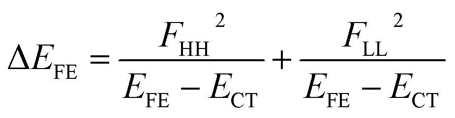 | (5) |
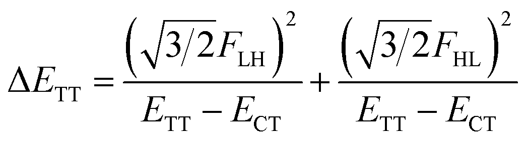 | (6) |
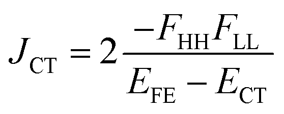 | (7) |
In order to estimate an approximate energy balance between the FE and TT states after the perturbation through the CT states, we defined the effective energy difference between them,58
| (ETT − EFE)eff = (ETT + ΔETT) − (EFE + ΔEFE − |Jeff|) | (8) |
A step-by-step view of this energy change by the perturbation through the CT states is shown in Fig. 1, where the effects of the energy corrections ΔEFE and ΔETT, together with the exciton–exciton splitting Jeff, related to Davydov splitting, are shown. The effective energy difference would represent whether the molecule could exhibit SF or TTA as an exothermic process. In Fig. 1, we show four cases in this study: strong mixing with the CT states both in FE and TT states (Fig. 1a), weak mixing with the CT states both in FE and TT states (Fig. 1b), strong mixing with the CT states in FE but not in TT (Fig. 1c), and strong mixing with the CT states in TT but not in FE (Fig. 1d). Note that eqn (8) is not the eigenvalue difference itself obtained from this effective Hamiltonian (eqn (2)) but should give the approximate relative energy balance between the FE-dominated and TT-dominated lowest excited eigenstates. Although Davydov splitting, which corresponds to 2|Jeff| in this dimer model, is widely used as a measure of the electronic coupling between chromophores, this does not give sufficient information for judging the possibility for SF and TTA. For SF and TTA, we need to know the non-horizontal couplings (FHL and FLH) that may be difficult to be extracted from UV/vis absorption spectrum. Also, we have to be careful that the strong electronic coupling estimated from only Davydov splitting might not indicate favourable situation for SF or TTA. Although the low-lying excited absorption bands actually includes the mixing of FE and TT states through VFE–TT, still it should be difficult to extract the coupling VFE–TT from Davydov splitting. Indeed, a recent theoretical study have shown negligible effects of the mixing with TT and FE states in the lowest lying absorption bands.64
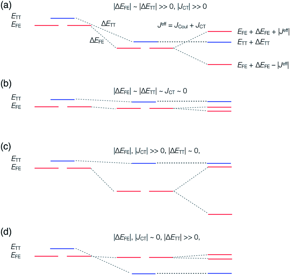 | ||
| Fig. 1 Energy diagram of singlet (FE) and triplet-pair (TT) states through charge-transfer (CT) states mixing. The case (I-PP), where the CT states strongly mix with both the FE and TT states, (a); the case (I-PN), where the CT states barely mix with both the FE and TT states, (b); the case (II-PP), where the CT states strongly mix with the FE states only, (c); the case (II-PN), where the CT states strongly mix with the TT state only, (d). See Section 2.3 for detail. | ||
We see that the energy stabilization in the FE state (ΔEFE and Jeff) is primarily caused by the horizontal couplings (FHH and FLL) appearing in eqn (5) and (7), while that in the TT state (ΔETT) by the non-horizontal couplings appearing in eqn (6). Therefore, if we could control each matrix element at will, we may address the desired energetic condition in a given chromophore. This issue is discussed in the rest part of this paper.
2.2 Electronic coupling in covalently-linked systems
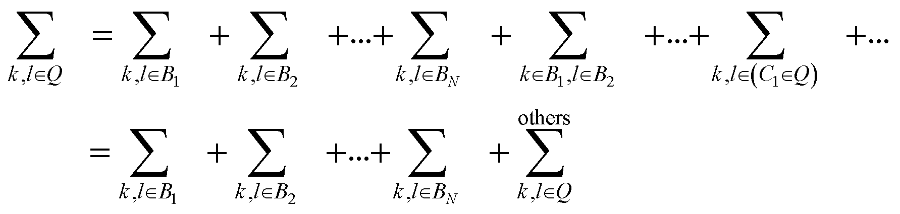
In covalently-linked dimer systems investigated in this study, we evaluate the Fock matrix elements in eqn (1) by using the non-orthogonal effective Hamiltonian theory.52,65,66 This is again an effective Hamiltonian theory as described in eqn (2) but the Hamiltonian considered here is the Fock matrix. Since the detail of the theory is not needed for discussion, we here describe only the essential part, which is directly related to both the present analysis and our molecular design strategy. The detail of the theory is found in the ESI† in the previous paper.52 The correspondence of the following treatment of electronic couplings to that in many-electron wavefunction theory has been pointed out by Zeng et al.63The orbital space spanned by atomic orbitals is divided into the subspace of interest called the model space P, which consists of the HOMOs and LUMOs of the chromophores, and the remaining subspace, called complement space Q, which consists of the rest of the MOs in the chromophores and in the bridges. The effective Fock operator as a function of the energy parameter (Fermi energy) E is written as
 | (9) |
![[Q with combining circumflex]](https://www.rsc.org/images/entities/i_char_0051_0302.gif) = †Ĉ1 + †Ĉ2 + = †Ĉ1 + †Ĉ2 + ![[B with combining circumflex]](https://www.rsc.org/images/entities/i_char_0042_0302.gif) 1 + 2 + … + N 1 + 2 + … + N
| (10) |
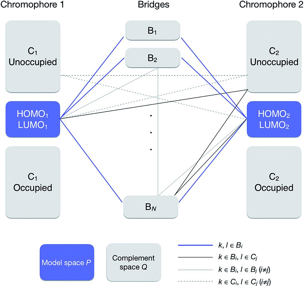 | ||
| Fig. 2 Orbital subspaces and interaction paths (see eqn (10) and (13)). Solid blue line represents the interaction paths from a MO to another MO in the model space through a bridge, solid thick grey line through a bridge and a chromophore, solid thin grey line through two bridges, and broken grey lines through two chromophores. All the grey line terms are included in terms named “others” in eqn (12). | ||
The quantum interference in a bridge-mediated coupling may be understood both by the atomic orbital picture and by MO picture. For the former, for example, see reviews.67–69 We here consider the MO picture, which is a hybrid view based on the use of localized MOs in each fragment (chromophores and bridges) and of delocalized MOs within a fragment.70 This picture is useful for describing the π-conjugated systems. We describe this at Hückel level of approximation as an introduction.52,70 For simplicity, we consider a singly-bridged chromophore dimer without direct-overlap, that is, two chromophores are spatially separated. In this level of approximation, the bridge-mediated coupling is expressed as52,70
 | (11) |
We here discuss the sign of the electronic couplings and how they are related to molecular structures. Let us consider a linear bridge with two π-orbitals like ethylene, a kind of alternant hydrocarbons. The top view of the HOMO and LUMO of the model bridge is schematically shown in Fig. 3a. Two chromophores are linked at the left and right sides of the bridge, respectively. This case should correspond to the constructive quantum interference as explained above. We further assume that the signs of the MOs of the chromophores are positive at the linked sites, which is always possible without losing the generality when we consider a singly-bridged system. Then, the bridge-mediated coupling should be positive because the prefactor of the parenthesis in eqn (11) is positive and the term in the parenthesis is also positive. Next, we consider another bridge with four π-orbitals in a line like butadiene. The Frontier MOs of such kind of compounds are shown in Fig. 3b. Again, two chromophores are linked with the bridge at the ends of the bridge, where constructive interference is also expected. Assuming the same situation as that of ethylene bridge in the relative phase of chromophores, we should obtain a negative coupling Fij, which is opposite to that obtained in the previous case, because the parenthesis term becomes negative. Consequently, we can predict the sign of the parenthesis term from the nature of π-orbitals in a bridge. The phase of bridge-mediated coupling is uniquely defined through the relative phase of the HOMO and LUMO of a bridge at the positions linked to the chromophores, which is an intrinsic property of a bridge. Thus, these two kinds of intrinsically constructive patterns realized in these bridges may be referred to as “positively-constructive (PC)” and “negatively-constructive (NC)”, respectively. When the two chromophore MOs have mutually the same signs at the linked sites, a PC bridge induces a positive coupling, while a NC bridge induces a negative coupling. On the other hand, when the two chromophore MOs have mutually the opposite signs at the linked sites, a PC bridge induces a negative coupling, while a NC bridge induces a positive coupling. Note that “positively-constructive” does not mean positive electronic coupling but does a positive value for the parenthesis term in eqn (11).
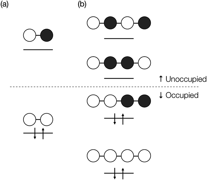 | ||
| Fig. 3 Top view of orbital diagram for linear two π-electron system such as ethylene (a), and for linear four π-electron system such as butadiene (b). The signs of the HOMO at the edges in the former have the same sign, while those in the latter have mutually the opposite sign. | ||
2.3 Doubly-bridged systems and quantum interference between bridges
In this section, we discuss the effect of quantum interference between N bridges, where the relative signs of the electronic couplings are quite important. By partitioning the complement space Q into subspaces as shown in eqn (10), the bridge-mediated contribution may be partitioned into the sum of the contributions from each subspace, that is, from each bridge (see also Fig. 2):
 | (12) |
 | (13) |
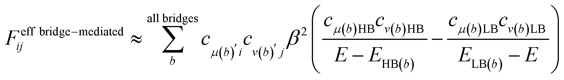 | (14) |
Here, we consider how the linked position affects the couplings, and then classifies all the situations, which are generated by considering the combination of the MO phases and bridge choices, into the four essential cases. We here consider only the symmetric doubly-bridged dimer (N = 2). All the signs of the eight chromophore MO coefficients appearing in the prefactor in eqn (14) for two bridges, cμ(1)′H1, cν(1)′H2, cμ(2)′H1, cν(2)′H2, cμ(1)′L1, cν(1)′L2, cμ(2)′L1 and cν(2)′L2, are related to the nature of the linked sites in the chromophores indicated, and the total patterns of them are 28 = 256 when we consider plus or minus for these coefficients. They, however, can be reduced into two situations when we consider only symmetric dimers. This is essentially sufficient to classify the effect of the bridges in electronic couplings studied here. The classification is based on the signs of the products of the MO coefficients in the chromophores at the linked sites. The first situation of the simplest ones is (I) that the products have the same signs in all the relevant combinations (Table 1). The second situation is somewhat complicated and is (II) that the products have the same signs in all the relevant combinations except for the two products, that is, the product of the HOMO of the chromophore 1 and the LUMO of the chromophore 2, and also the product of the LUMO of the chromophore 1 and the HOMO of the chromophore 2, at the linked sites of only one of the bridges (Table 2). In the ESI,† we show some examples of seemingly different but physically equivalent situations with that shown in Table 1. In addition to these essential two MO phase patterns in the chromophores at the linked sites, four ways of the choices in the bridge character are possible: PC–PC, NC–NC, PC–NC, and NC–PC, which indicate the character of bridge 1–2, respectively. However, these four choices in the bridge character again can also be reduced into two, because the others give the essentially same electronic couplings except for their sign, which does not change the underlying physics. For example, the bridge choice of PC–PC gives the same electronic coupling matrix elements in their amplitudes with the opposite signs to those from the corresponding bridge choice NC–NC, given the MO amplitudes in the bridge moieties are the same. Thus, we do not distinguish them in this paper. In total, we have four cases in symmetric doubly-bridged dimers: (I-PP) the chromophore MO phases at the linked sites are in the pattern (I) and the combination of the bridges is PC–PC; (I-PN) the chromophore MOs are in the pattern (I) and the combination of the bridges is PC–NC; (II-PP) the chromophore MOs are in the pattern (II) and the combination of the bridges is PC–PC; (II-PN) the chromophore MOs are in the pattern (II) and the combination of the bridges is PC–NC. As noted above, we refer to the case that is called (I-NN) as (I-PP).
| H2@b1 | H2@b2 | L2@b1 | L2@b2 | |
|---|---|---|---|---|
| a Hi@bj (Li@bj) represents an index of the MO coefficient of the HOMO (LUMO) of the chromophore i at the linked site with the bridge j, cμ(j)′Hi (cμ(j)′Li).b + indicates the positive sign of the product of MO coefficients of the chromophore 1 shown in the left column and of 2 shown in the top row. Blank cells represent that any signs of the product are possible for this case. | ||||
| H1@b1 | + | + | ||
| H1@b2 | + | + | ||
| L1@b1 | + | + | ||
| L1@b2 | + | + | ||
| H2@b1 | H2@b2 | L2@b1 | L2@b2 | |
|---|---|---|---|---|
| a Hi@bj (Li@bj) represents an index of the MO coefficient of the HOMO (LUMO) of the chromophore i at the linked site with the bridge j, cμ(j)′Hi (cμ(j)′Li).b + and − indicate the positive and negative signs of a product of the MO coefficients of the chromophore 1 shown in the left column and of 2 shown in the top row, respectively. Blank cells represent that any signs of the product are possible for this case. | ||||
| H1@b1 | + | + | ||
| H1@b2 | + | − | ||
| L1@b1 | + | + | ||
| L1@b2 | − | + | ||
The above essential four cases, that is, (I-PP), (I-PN), (II-PP) and (II-PN), are schematically shown in Fig. 4. Other cases that are not shown in Fig. 4 are physically equivalent to one of them, or are non-symmetric dimers, or are other linking patterns (see below). In Fig. 4, the phases of the HOMO and LUMO at the linked sites are expressed by white (positive) and black (negative) circles. A PC and NC are denoted by solid and broken lines, respectively. In the case (I-PP), in all the Fock matrix elements Fij, the quantum interference between bridges is constructive, leading to large electronic coupling amplitudes in all the elements. In the case (I-PN), the situation is opposite: in all the Fock matrix elements Fij, the quantum interference between bridges is destructive, leading to small electronic coupling amplitudes in all the elements. In the case (II-PP), due to the PC nature of the bridges 1 and 2 and mutually anti-phase HOMO–LUMO relation of chromophores at the two linked sites, constructive interference in horizontal couplings (FHH and FLL) results in large amplitudes of them, while destructive interference in non-horizontal couplings (FHL and FLH) results in small amplitudes of them. In the case (II-PN), the situation is opposite to the previous case: destructive interference in horizontal couplings results in small amplitudes of them, while constructive interference in non-horizontal couplings results in large amplitudes of them. In short, it is found that in the case (I-PP) (in the case (I-PN)), all the Fock matrix elements are large (small) in their amplitudes; in the case (II-PP) (in the case (II-PN)), the horizontal couplings are large (small) in their amplitudes, while the non-horizontal couplings are small (large) in their amplitudes.
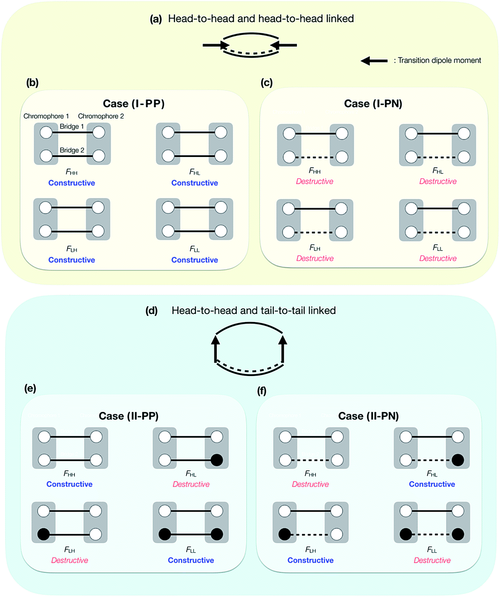 | ||
| Fig. 4 Schematic picture of bridge linked patterns with head-to-head and head-to-head positions (concerning the transition dipole moments of chromophores) (a), and with heat-to-head and tail-to-tail positions (d), and of quantum interference between bridges in the cases (I-PP), (I-PN), (II-PP) and (II-PN) ((b), (c), (e) and (f)). Two chromophores (grey rectangular part) are linked by two bridges (black solid and/or broken lines). The phases of HOMO and LUMO at the linked sites are indicated by white (positive) and black (negative) circles. A positively-constructive and negatively-constructive bridges are described as black solid and broken lines, respectively. | ||
We give some comments on the characteristics and the potential for materials design using these four cases. The case (I-PP) seems to be a simple extension of singly-bridged systems, where the effect of a bridge is doubled when the same bridges are used. The difference between the singly-bridged systems and I-(PP) will be shown in ab initio calculations in this paper. The case (I-PN) may be a good way to design weak coupling system, which could lead to slow but high-yield SF and/or TTA systems.47,52,56,63 The lowest lying state can keep its electronic character from strong mixing with other states due to small electronic couplings from the view point of electronic configuration. At the same time, small electronic couplings, however, would suppress the transition rate between the FE and TT states, and could lead to deactivation pathways for the system before undergoing SF or TTA. This is an issue of dynamics, so that quantum dynamics simulation or rate estimation will answer the question of whether a system prefers. We do not discuss in detail this issue because we focus mainly on qualitative difference in electronic couplings and resulting energetics, and this is beyond the scope of the present paper. The cases (II-PP) and (II-PN) may be interesting because, from eqn (5)–(7), the relative energy balance between singlet and triplet-pair excited states eqn (8) may be controlled by tuning the relative amplitude of the horizontal and non-horizontal couplings. These four cases are expected to correspond to the energy diagrams shown in Fig. 1a–d, respectively.
As noted above, Fig. 4 does not cover all the patterns of MOs in symmetric doubly-bridged systems, though other patterns are physically equivalent to one of the above four cases. In fact, the case (I-PP), which results in constructive quantum interferences in all the Fock matrix elements, is also found for other phase patterns of MOs, see Fig. S1.† This complexity may be avoided by considering the direction of the transition dipole moment of the HOMO to LUMO transition in a chromophore, which provides information of the relative phase of the MO, instead of the phases of MOs themselves. Schematic pictures of the relative direction of the transition dipole moments in the chromophores are shown in Fig. 4a and d, the former of which correspond to the cases (I-PP) and (I-PN), and the latter of which correspond to the cases (II-PP) and (II-PN), respectively. In this viewpoint, the cases (I-PP) and (I-PN) correspond to linking the chromophores at two head-to-head positions concerning the transition dipole moments of the chromophores, respectively, while the case (II-PP) and (II-PN) correspond to bridging at head-to-head and tail-to-tail positions. More precisely, local distribution of the transition density is found to classify the effects of the linked position into the cases (I-PP) and (I-PN), and into (II-PP) and (II-PN). This is approximately identified by taking a product of the HOMO and LUMO of the chromophore, which turns out to be identical to considering the relative phase of the MOs at the linked positions shown in Fig. 4. Other cases rather than these four cases, for example, asymmetrically bridged, triply- and multiply-bridged systems, head-to-tail bridged systems, and hetero dimer53,55 systems are possible and interesting, though we do not go further in this study. Electronic couplings in such systems can also be predicted in the same manner.
3 Model systems
We choose tetracene as the model chromophore in this study (Scheme 1a). Tetracene is known to have a slightly lower singlet excitation energy E(S1) = 2.32 eV than twice the triplet excitation energy 2E(T1) = 2.50 eV in crystal,71 while in gas phase, the singlet excitation energy is estimated to be 2.75–2.76 eV![[thin space (1/6-em)]](https://www.rsc.org/images/entities/char_2009.gif) 41,72 (see Section 4), which is 0.25–0.26 eV higher than twice the triplet excitation energy. The quantum yield of the fluorescence of unsubstituted tetracene in solution is reported as 14–16%,73 and it reaches up almost unity by changing substituents.74 On the contrary, in solid phase, tetracene and its derivatives are known to induce high-yield SF13–19 with providing essentially no fluorescence (2 × 10⁻⁵% quantum yield75). This approximate isothermic condition of tetracene for SF and TTA motivates us to investigate the possibility of selective control of the Fock matrix elements suitable for SF or TTA on the basis of the perturbation analysis in Section 2.1. The product of the HOMO and LUMO, which represents the approximate transition density, is found to be positive on the one of the zigzag edge, while negative on the other zigzag edge (see the ESI†). Hence, we expect that the cases (I-PP) and (I-PN) could be realized when two tetracenes are linked by two bridges at the same side of the zigzag edge carbon atoms, and that the cases (II-PP) and (II-PN) could be realized when linked at the armchair edge carbon atoms. We consider polyyne with n ethynyl units as a bridge. Polyynes can be utilized for linking covalently many kinds of chromophores with different ethynyl unit lengths.76–82 As in the cases of polyene bridges discussed in Section 2.2, a polyyne also should act as a PC bridge when odd n = 1, 3, 5, …, and a NC bridge when even n = 2, 4, 6, …. By using two polyynes with the lengths m and n, we consider two model dimers 1-(m, n), where the chromophores are linked through the polyynes at C1 and C10 atoms, and 2-(m, n), where the chromophores are linked through the polyynes at C2 and C3 atoms (see Scheme 1b). For comparing the performance of the model dimer with others reported in previous studies, we also consider ortho-bis(5-ethynyltetracenyl)benzene (BET-B). This molecule was shown to undergo SF very efficiently with the triplet yield 1.54 ± 0.10 (1.54 triplet excitons per singlet exciton) with the time constant of 2 ps in its thin film,49 which is the highest triplet yield and the fastest SF in covalently-linked tetracene dimers reported ever.41,42,46,49
41,72 (see Section 4), which is 0.25–0.26 eV higher than twice the triplet excitation energy. The quantum yield of the fluorescence of unsubstituted tetracene in solution is reported as 14–16%,73 and it reaches up almost unity by changing substituents.74 On the contrary, in solid phase, tetracene and its derivatives are known to induce high-yield SF13–19 with providing essentially no fluorescence (2 × 10⁻⁵% quantum yield75). This approximate isothermic condition of tetracene for SF and TTA motivates us to investigate the possibility of selective control of the Fock matrix elements suitable for SF or TTA on the basis of the perturbation analysis in Section 2.1. The product of the HOMO and LUMO, which represents the approximate transition density, is found to be positive on the one of the zigzag edge, while negative on the other zigzag edge (see the ESI†). Hence, we expect that the cases (I-PP) and (I-PN) could be realized when two tetracenes are linked by two bridges at the same side of the zigzag edge carbon atoms, and that the cases (II-PP) and (II-PN) could be realized when linked at the armchair edge carbon atoms. We consider polyyne with n ethynyl units as a bridge. Polyynes can be utilized for linking covalently many kinds of chromophores with different ethynyl unit lengths.76–82 As in the cases of polyene bridges discussed in Section 2.2, a polyyne also should act as a PC bridge when odd n = 1, 3, 5, …, and a NC bridge when even n = 2, 4, 6, …. By using two polyynes with the lengths m and n, we consider two model dimers 1-(m, n), where the chromophores are linked through the polyynes at C1 and C10 atoms, and 2-(m, n), where the chromophores are linked through the polyynes at C2 and C3 atoms (see Scheme 1b). For comparing the performance of the model dimer with others reported in previous studies, we also consider ortho-bis(5-ethynyltetracenyl)benzene (BET-B). This molecule was shown to undergo SF very efficiently with the triplet yield 1.54 ± 0.10 (1.54 triplet excitons per singlet exciton) with the time constant of 2 ps in its thin film,49 which is the highest triplet yield and the fastest SF in covalently-linked tetracene dimers reported ever.41,42,46,49
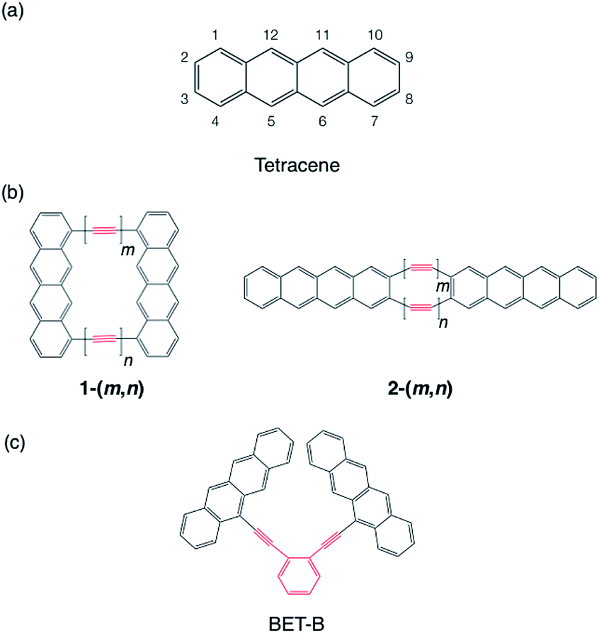 | ||
| Scheme 1 Molecular structure tetracene (a), model tetracene dimers (b) and experimentally investigated tetracene dimer (c).49 Here, (m, n) = (1, 1), (2, 1), (2, 2), (3, 1), (3, 2) and (3, 3). BET-B = ortho-bis(5-ethynyltetracenyl) benzene. Bridge moieties are indicated by red lines. | ||
4 Computational details
Molecular geometries were optimized by using density functional theory with the Grimme's dispersion correction B97-D xc-functional83 at their highest possible point group, except for 1-(1,1), where the D2h geometry was found to have an imaginary frequency and thus reduced to C2h. The long-range correction scheme84 combined with the Becke–Lee–Yang–Parr exchange–correlation functional84,85 (LC-BLYP) was used for the electronic coupling calculations, where the range-separating parameter μ is set to 0.33 bohr−1.86 The electronic couplings were evaluated by using eqn (9). The Frontier MOs in the chromophores were obtained through the diagonalization of the Fock matrix, which is evaluated in the whole molecule, in the subspace of each fragment, that is, C1, C2, B1 and B2, respectively, as was done in the previous study.52 In order to evaluate JCoul, we considered hydrogen-capped chromophores. After the geometry optimization in the model molecules 1-(m, n) and 2-(m, n), the bridge moiety (polyyne part) and the other chromophore are removed, and two hydrogen atoms are attached onto the remaining tetracene moiety instead of the removed parts. The position of attached hydrogen atoms were optimized under the restriction of the other atoms being fixed. After this, JCoul was computed from the Coulomb interaction between the Mülliken transition atomic charges obtained from the time-dependent density functional theory calculation using LC-BLYP for each isolated tetracene, as was done in the previous study.58 Pople's 6-31G** basis set87 was used for all the calculations. All the quantum chemistry calculations were performed by using Gaussian 09 program package.88 The effective Hamiltonian matrix elements were evaluated by using our house code.The relative energy of the FE and TT states is crucial for determining whether SF or TTA tends to occur. Here, we consider the 0–0 absorption band energy for state X relative to the ground state as
| EX = EFCX + EvibX + EpolX + EmixX | (15) |
71 is expected to be regarded as an approximation to E(T) without EmixX. Hence, we set ETT = 2E(T) = 2.50 eV in eqn (1).
The singlet excited state 0–0 absorption band excluding the polarization effect, that is, the excitation energy in gas phase, can be estimated as ES1(gas) = 2.75–2.76 eV41,72 by combining the solution spectra and empirical correction for solvation effect (ES1(gas) = ES1(solution) + Δsol).95 Typical values of this correction, which may be regarded as the polarization effect in solution, for the HOMO–LUMO singly-excited singlet state of polyaromaric hydrocarbons range 900–1500 cm−1 = 0.11–0.19 eV depending on solvents.95 Here, we consider this correction for ES1(gas) in order to obtain a balanced treatment both for singlet and triplet exciton, where the latter ET1 = 1.25 eV includes the polarization effect in condensed phase. We set the correction as 0.15 eV, and hence, EFE (including polarization effect) = 2.76–0.15 = 2.61 eV, where the solvent effect corresponds to benzene solution. Consequently, we assume slightly higher energy of FE state than TT state, ETT − EFE = −0.11 eV. This means that SF is exothermic, while TTA is endothermic in the weak electronic coupling limit, that is, EmixX = 0.
The location of the CT state energy is still under debate. The electroabsorption spectra in tetracene crystal gave ECT = 2.71–3.063 eV,96 depending on the dimer-pairs in crystal. Using these values, theoretical modelling including FE and CT states with vibronic effect succeeded in reproducing the absorption spectra in tetracene crystal.97 Although it can be different for each dimer, we assume ECT = EFE + 0.3 = 2.91 eV, which is in above values, for all the dimers. The CT energy dependence will be discussed in Section 5.4, otherwise the CT energy is fixed at 2.91 eV.
5 Results and discussion
5.1 Fock matrix element
Table 3 represents the evaluated electronic couplings of the dimers 1-(m, n) and 2-(m, n). Obviously, in 1-(m, n), in the even combinations, that is, m + n = even, all the Fock matrix elements are found to be large and to lie in the range of 118.3–334.6 meV in their amplitudes except for FLL in 1-(1, 1), while in the odd combinations, that is, m + n = odd, they are found to be relatively small and to lie in the range of 13.9–63.7 meV. This is what we expected from our discussion in Section 2.3, and the even and odd combinations should correspond to the cases (I-PP) and (I-PN), respectively. We note that the difference between FHH and FLL, which is important for large VFE–TT, is also large for the case I-(PP). This is explained by the doubling of the residue terms from the next-nearest-neighbour interaction.52| Molecule | Horizontal coupling | Non-horizontal coupling | ||
|---|---|---|---|---|
| FHH | FLL | FHL | FLH | |
| 1-(1, 1) | 334.6 | −89.6 | 284.8 | 284.8 |
| 1-(2, 1) | 63.7 | 38.9 | 44.4 | 44.4 |
| 1-(2, 2) | −247.8 | −154.5 | −237.2 | −237.2 |
| 1-(3, 1) | 285.0 | 176.7 | 251.6 | 251.6 |
| 1-(3, 2) | −34.9 | −13.9 | −37.0 | −37.0 |
| 1-(3, 3) | 188.8 | 118.3 | 160.7 | 160.7 |
| 2-(1, 1) | 263.4 | 291.6 | 0.0 | 0.0 |
| 2-(2, 1) | 58.5 | 20.9 | −239.7 | −239.7 |
| 2-(2, 2) | −180.0 | −181.9 | 0.0 | 0.0 |
| 2-(3, 1) | 214.0 | 175.8 | −72.1 | −72.1 |
| 2-(3, 2) | −26.7 | −12.8 | 170.3 | 170.3 |
| 2-(3, 3) | 139.1 | 129.1 | 0.0 | 0.0 |
By changing the linked pattern between chromophores and bridges from that of 1-(m, n), 2-(m, n) shows large horizontal couplings of 129.1–291.6 meV and small non-horizontal couplings 0–72.1 meV in their amplitudes in the even combinations, while shows small horizontal couplings 12.8–58.5 meV and large non-horizontal couplings 170.3–239.7 meV in their amplitudes in the odd combinations. These even and odd combinations in 2-(m, n) should correspond to the cases (II-PP) and (II-PN), respectively.
Here we have clearly demonstrated that we can design horizontal and non-horizontal couplings separately through tuning the bridge character, PC–NC, and the linked position. In order to confirm the correspondence between the results shown in this section and the theory provided in Section 2.3, we perform a further analysis of these couplings in the next section.
5.2 Decomposition analysis
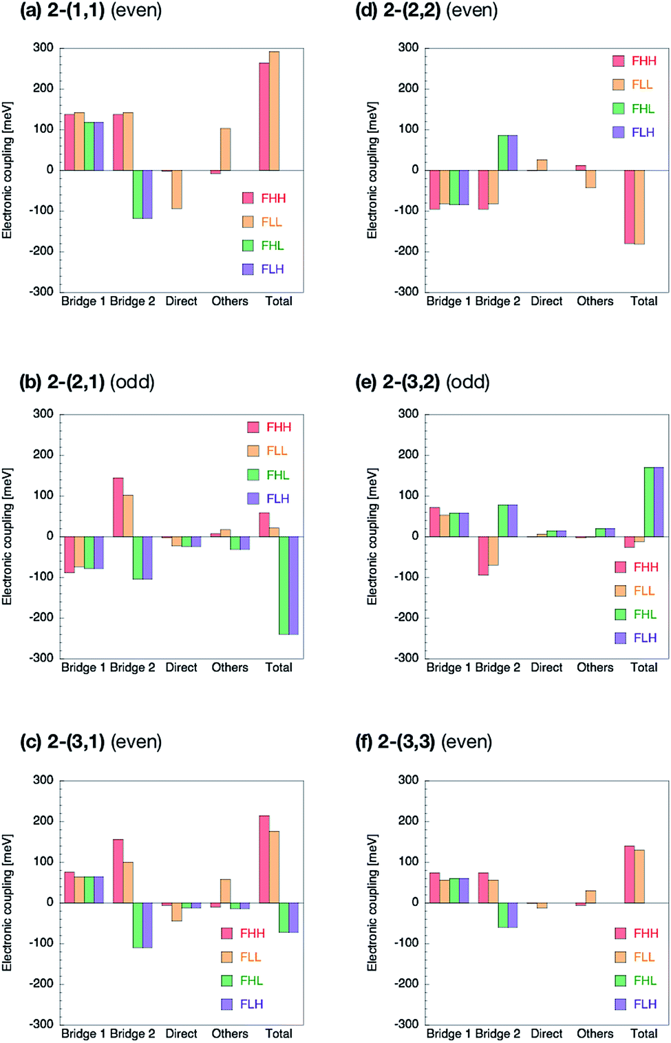
The Fock matrix elements, both horizontal and non-horizontal couplings, are decomposed into the direct-overlap contribution, each bridge-mediated contribution and other contributions by using eqn (10) and (12). Here only bridge π-orbitals are considered as the bridge orbital subspaces. The results are shown in Fig. 5 for 1-(m, n) and Fig. 6 for 2-(m, n). The results show clear relationship between the Fock matrix elements, even–odd combinations and linked positions. In all the (m, n) combinations of 1 and 2, each bridge-mediated coupling within a bridge is shown to be constructively enhanced, resulting in their large amplitudes. However, the signs of a coupling for a bridge as well as for the other bridge depend on (m, n) combinations and the linked positions of the fragments. This is the quantum interference between bridges. In 1-(m, n) with the even combination, all the Fock matrix elements are found to be enhanced through constructive quantum interference between the bridges (Fig. 5a, c, d and f), while in the odd combination of 1-(m, n), all the Fock matrix elements are found to be suppressed by destructive quantum interference (Fig. 5b and e). Therefore, these are considered to correspond to the cases (I-PP) and (I-PN), respectively. Note that 1-(1, 1) has non-negligible contribution from direct-overlap contribution and has contribution other than the bridges. This might be due to distortion of the π-plane in the chromophores, and also be related to the sensitivity to the localization method used to evaluate the couplings in the previous study.98 Enormous contributions in FLL other than direct and π-orbital bridge-mediated terms is partly due to non-negligible interactions with σ-orbitals of bridges (see ESI†). To resolve this strange behaviour for such a kind of compounds, we might need further development of the present theory, which is left for the future investigation.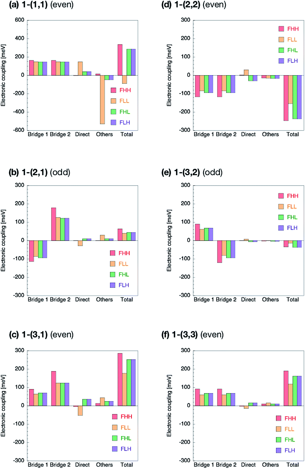 | ||
| Fig. 5 Decomposition of the Fock matrix elements in 1-(m, n) into the two bridge-mediated contributions from the bridges 1 and 2, direct-overlap contribution, and others. Here, (m, n) = (1, 1) (a), (2, 1) (b), (3, 1) (c), (2, 2) (d), (3, 2) (e), and (3, 3) (f). The longer bridge is referred to as bridge 1. | ||
 | ||
| Fig. 6 Decomposition of the Fock matrix elements in 2-(m, n) into the two bridge-mediated contributions from the bridges 1 and 2, direct-overlap contribution, and others. Here, (m, n) = (1, 1) (a), (2, 1) (b), (3, 1) (c), (2, 2) (d), (3, 2) (e), and (3, 3) (f). The longer bridge is referred to as bridge 1. | ||
The situation is quite different in 2-(m, n). In the even combinations (Fig. 6a, c, d, and f), we find that the horizontal couplings have the same sign contributions from both the bridges, while the non-horizontal couplings have the mutually opposite sign contributions from each bridge. On the contrary, in the odd combinations (Fig. 6b and e) we find that the horizontal couplings have the mutually opposite sign contributions from each bridge, while the non-horizontal couplings have the same sign contributions from both the bridges. As a result, it is found that the even combinations in 2-(m, n) give the large horizontal and small non-horizontal couplings, while that the odd combinations do the small horizontal and large non-horizontal couplings. The even and odd combinations in 2-(m, n) should correspond to the cases (II-PP) and (II-PN), respectively.
Zero non-horizontal couplings in 2-(n, n) (m = n), that is, the sum of the direct, bridge-mediated and other terms in them, may also be explained and understood by symmetry. Note that the point group of localized diabatic wavefunctions such as the HOMO and LUMO of chromophores in 2-(n, n) no longer belongs to the D2h point group but to C2v point group, where the C2 rotation axis lies along the long axis of the molecule. Therefore, the HOMO of a chromophore belongs to the A2 irreducible representation and the LUMO of the other chromophore belongs to the B1 irreducible representation in the C2v point group, respectively, so that the Fock matrix elements FHL and FLH vanish. A role of symmetry in covalently-linked SF systems was also discussed in several papers.1,2,23,45,92 Unfortunately, although this explanation based on symmetry gives a clear insight into a part of electronic couplings in covalently-linked systems, this is not sufficient for other compounds and for horizontal couplings investigated in the present study. For example, smaller non-horizontal coupling in 2-(3, 1) than 2-(3, 2) in spite of shorter bridge length of the former cannot be explained by symmetry nor in an intuitive way. The comprehensive understanding of the difference in the electronic couplings between these compounds 1-(m, n) and 2-(m, n) should be accomplished through the consideration of the quantum interference.
5.3 Perturbation analysis
In this section, we provide the perturbation analysis of model systems of the cases (I-PP), (I-PN), (II-PP) and (II-PN) in order to clarify the effect of electronic couplings on the energetics. As shown in eqn (5)–(8) as well as in Fig. 1, the relative energy of the FE and TT states after the CT-mixing through the horizontal and non-horizontal couplings strongly depends on the coupling strength and the CT state energy. Here, we have fixed the CT state energy as 2910 meV, which is 300 meV higher than FE state. The evaluated second-order contributions to the FE and TT state energies as well as to the excitonic coupling are summarized in Table 4. The even–odd parity dependence on each energy correction, coupling and energetics are summarized in Table 5.| 1-(m, n) | 2-(m, n) | ||||||
|---|---|---|---|---|---|---|---|
| n | n | ||||||
| 1 | 2 | 3 | 1 | 2 | 3 | ||
| a Eqn (8). | |||||||
| ΔEFE | |||||||
| m | 1 | −566.9 | −514.7 | ||||
| 2 | −29.3 | −284.2 | −12.8 | −218.3 | |||
| 3 | −374.9 | −4.7 | −165.4 | −255.6 | −2.9 | −120.0 | |
|
|||||||
| ΔETT | |||||||
| m | 1 | −593.4 | 0.0 | ||||
| 2 | −58.8 | −411.7 | −420.5 | 0.0 | |||
| 3 | −169.0 | −10.0 | −188.8 | −38.0 | −212.2 | 0.0 | |
|
|||||||
| JCoul | |||||||
| m | 1 | 23.4 | 1.4 | ||||
| 2 | 14.8 | 9.0 | 1.8 | 0.8 | |||
| 3 | 10.4 | 6.3 | 4.4 | 3.3 | 0.9 | 0.5 | |
|
|||||||
| JCT | |||||||
| m | 1 | −199.9 | 512.0 | ||||
| 2 | 16.5 | 255.3 | 8.1 | 218.3 | |||
| 3 | 335.7 | 3.2 | 148.9 | 250.7 | 2.3 | 119.6 | |
|
|||||||
| VFE–TT | |||||||
| m | 1 | 427.0 | 0.0 | ||||
| 2 | 3.9 | 78.2 | −31.9 | 0.0 | |||
| 3 | 96.4 | 2.8 | 40.0 | −9.7 | −8.4 | 0.0 | |
|
|||||||
| (ETT − EFE)effa | |||||||
| m | 1 | 40.1 | 918.1 | ||||
| 2 | −108.1 | 26.9 | −507.7 | 327.3 | |||
| 3 | 441.9 | −105.8 | 19.8 | 361.6 | −316.1 | 130.1 | |
| Parity | Case | Horizontal coupling | Non-horizontal coupling | |ΔEFE|, |JCT| | |ΔETT| | Lowest state expected |
|---|---|---|---|---|---|---|
| a CT energy sensitive.b Assuming the condition ETT < EFE at the monomer level. | ||||||
| Even | (I-PP) | Large | Large | Large | Large | FE/TTa |
| Odd | (I-PN) | Small | Small | Small | Small | TTb |
| Even | (II-PP) | Large | Small | Large | Small | FE |
| Odd | (II-PN) | Small | Large | Small | Large | TT |
First, we discuss the results of the perturbation analysis in 1-(m, n) (see Table 4). The amplitude of the energy correction to the FE state through the CT-mixing, ΔEFE, is found to be moderate in its amplitude for all the even combinations, while small for all the odd combinations. The order in the amplitude is, 1-(1, 1) (ΔEFE = −566.9 meV) > 1-(3, 1) (−374.9 meV) > 1-(2, 2) (−284.2 meV) > 1-(3, 3) (−165.4 meV) > 1-(2, 1) (29.3 meV) > 1-(3, 2) (−4.7 meV). It is found that longer bridges give less correction than short one 1-(1, 1) does when m = n. The energy correction to the FE state is found to be much more significant for even combinations than for odd combinations by one to two orders in its magnitude. The energy correction to the TT state, CT-mediated excitonic coupling JCT and FE–TT coupling VFE–TT are found to have the same even–parity dependence as that to the FE state. Hence, the electronic transition between the FE and TT states, that is, SF or TTA, is expected to be faster in the even combinations than odd combinations of 1-(m, n). The Coulomb contribution in the excitonic coupling, JCoul, is found to be much smaller than JCT in the even combinations. The effective energy difference defined by eqn (8) is shown to be positive for all the even combinations and negative for odd combinations, which indicates that the former molecules favour TTA rather than SF, while the latter favour SF rather than TTA.
Next, we discuss the results of the perturbation analysis in 2-(m, n) (see Table 4). The amplitude of the energy correction to the FE state |ΔEFE| is found to be moderate in its amplitude for all the even combinations, while small for all the odd combinations. This seems to be the same as the situation found in 1-(m, n). The CT-mediated excitonic coupling JCT, which is found to be much larger than JCoul, shows the same tendency as the energy correction to the FE state ΔEFE. In contrast to ΔEFE and JCT, which are significant in the even combinations in both 1-(m, n) and 2-(m, n), the energy correction to the TT state ΔETT in 2-(m, n) shows the opposite tendency in the even–odd parity; the odd combinations have much larger |ΔETT| than that of the even combinations. The FE–TT coupling is found to be the largest in the odd combination 2-(2, 1) (|VFE–TT| = 39.1 meV), the second largest in 2-(3, 1) (9.7 meV) and then 2-(3, 2) (8.4 meV). We see that the even combinations with m = n have no VFE–TT due to zero non-horizontal couplings as shown above. We find that the effective energy difference in 2-(m, n) is positive in even combinations, while negative in odd combinations. This is considered as the result from the difference in the even–odd parity dependence between the horizontal-coupling-induced terms (|ΔEFE| and |JCT|) and the non-horizontal-coupling-induced term (|ΔETT|), where the former two terms are found to be large in the even combinations, while the latter term is found to be large in the odd combinations (see Table 5). From these considerations, we expect that the lowest excited state of the even combination molecules of 2-(m, n) tends to become FE dominated and therefore favours TTA rather than SF, while that of the odd combination molecules of 2-(m, n) tends to become TT dominated and therefore favours SF rather than TTA.
It is interesting to compare the present model molecules with previously reported efficient SF systems in order to clarify the applicability of the present approach. In contrast to most previous studies on covalently-linked tetracene dimers,41,42,46 which reported that the SF is endothermic and thereby inefficient, Korovina et al. reported that highly efficient SF in the covalently-linked tetracene dimer, BET-B, see Scheme 1.49 The SF time constant and triplet yield were reported to be in the range of 0.8–2 ps depending on the media and 154 ± 10%, respectively.49 Its efficient SF was also confirmed by theoretical calculations, which indicate that the strong electronic coupling pushes the TT state below the FE state.50 In order to compare our model molecules with this result, we evaluate the Fock matrix elements, energy correction and effective coupling matrix elements of BET-B (see Table 6). Clearly, we see the large non-horizontal couplings as compared to the horizontal ones, the formers of which mainly originate from the direct-overlap contribution (see the ESI†), indicating a much stronger stabilization in the TT state than in the FE state. As expected, the effective energy difference is largely negative, (ETT − EFE)eff = −1730.6 meV, which corresponds to energetically favourable SF. Besides, we also find the large VFE–TT = 390.8 meV. Judging from these results, we conclude that highly efficient SF in BET-B is due to these large non-horizontal couplings as compared to the horizontal couplings, which favour the energetically exothermic condition, and due to the large VFE–TT, which induces very fast SF. Of course, we cannot expect nearly 2 eV stabilization through the electronic coupling in the TT state, which is clearly beyond the perturbation region. Despite that, we certainly obtained qualitative agreement with the experiment49 and the theoretical calculation50 with more sophisticated methodology. This example highly motivates us to further investigate the possibility of our designed molecules, especially the case (II-PN) (2-(2, 1) and 2-(3, 2)) for SF, where the non-horizontal couplings are much larger than the horizontal couplings. This is in the same situation as the case of BET-B, though here we have achieved that through the control of bridge-mediated contribution. Although the coupling, VFE–TT, and exothermicity |(ETT − EFE)eff| are small as compared to those in BET-B, fast SF is expected for both of them (τSF = 120–300 ps in 2-(2, 1) and 1.7–4.3 ns in 2-(3, 2)), by optimistically assuming that the SF rate is proportional to the square of VFE–TT with exothermic conditions (τSF/τBET-BSF = |VFE–TT/VBET-BFE–TT|2). These are still two or three orders faster than the previously reported low yield tetracene dimers. As previously reported non-radiative and radiative decay time constants for most tetracene dimers are in the order of ten nanoseconds,42,46,49 2-(2, 1) and 2-(3, 2) should be promising candidates for SF, though a faster non-radiative decay in 500 ps was reported for BET-B.
| ΔEFE | ΔETT | JCoul | JCT | VFE–TT | (ETT − EFE)eff |
|---|---|---|---|---|---|
| −232.0 | −1955.5 | 23.5 | 79.5 | 390.8 | −1730.6 |
We note an interesting point in the effective energy difference eqn (8) for covalently-linked systems. Using rough but reasonable approximations (see the ESI†), we can show that the effective energy difference is always higher than the energy difference without the CT-mixing,
| (ETT − EFE)eff > ETT − EFE(=−0.11 eV) | (16) |
This is derived for covalently-linked dimers with a constructive bridge, two constructive bridges of the cases (I-PP) and (II-PP), where these cases give large amplitudes in all or horizontal part of the Fock matrix elements, and of the case (I-PN), where all the Fock matrix elements are small. This relationship (eqn (16)) seems to hold certainly in the cases (I-PP), (I-PN) and (II-PP) investigated here. The inequality eqn (16) indicates that TTA is much easier to achieve its energetic requirement than SF in covalently-linked dimers. At the same time, it is also shown that our strategy of using multiple bridges, which breaks eqn (16), is a powerful tool for realizing SF exothermically. Indeed, this has been achieved in the case (II-PN), where only the non-horizontal couplings are enhanced and breaks eqn (16). Eqn (16) seems also consistent with the results of previous SF studies, where most tetracene dimers41,42,44–46 and crystals15,18–20,22,25,26 show the endothermic behaviours except for BET-B.49
Finally, we examine the above perturbation analysis through the full diagonalization of the Hamiltonian eqn (1), see the ESI,† where the relative eigenenergies and main characters of the eigenstates are presented (Fig. S9 and S10†). We find good agreement between the perturbative analysis and the full diagonalization in both the energies and characters in the cases of odd combinations of 1-(m, n), and of odd and even combinations of 2-(m, n). However, in the result of full diagonalization, we also find that the even combinations of 1-(m, n) have the lowest excited eigenstates mainly composed of TT character, which are different from those predicted by the perturbative analysis. In the even combinations of 1-(m, n), all the electronic couplings Fij are large in their magnitudes, and thus they might induce a difficulty in the perturbation approximation. Both FE dominated and TT dominated states are found to be significantly stabilized through the mixing with CT states in these compounds, and thus in such a case a variational calculation may be inevitable. From these results, we conclude that the perturbative approach (eqn (8)) can predict the consistent character of the lowest excited state with that obtained from variational calculations except for the case where both horizontal and non-horizontal couplings are significantly large with similar amplitudes. We also confirm the stabilization of the TT state in 2-(2, 1) and 2-(3, 2) is not so much as to slow down SF and as to prohibit the TT state from separating into free triplets.99 We have also performed the full diagonalization for BET-B, and obtained the lowest eigenstate dominated by TT state (55.8%) followed by CT state (41.8%). The TT dominated eigenstate was lower in its energy than the next lowest eigenstate dominated by FE character by 647.8 meV. Again, we see a qualitative agreement between the results obtained from perturbative and variational approaches.
5.4 CT state energy dependence
In the previous section, we discussed the perturbation analysis based on the fixed energy in the CT state, 2.91 eV, 0.3 eV higher than the FE state. Here, we consider the CT state energy dependence because the CT state energy is known to be sensitive to the environment, which might change the discussion in the previous section. In Fig. 7, we show the effective energy differences (ETT − EFE)eff in 1-(m, n) and 2-(m, n) as a function of the relative CT energy ECT − EFE. Other CT-mediated terms are also shown in the ESI.† We find significant CT energy dependence in all the molecules except for odd combinations of 1-(m, n), where all the Fock matrix elements are small, especially in the small ECT region. The effective energy difference in the even combinations of 1-(m, n) is found to change from positive to negative values as the relative CT energy ECT − EFE goes up from 300 to 400 meV. This indicates that the lowest excited state in the even combinations of 1-(m, n) is highly sensitive to the CT state energy, which depends on the environmental condition such as solvent or crystal field effect. This implies that the FE–CT and TT–CT mixings indicated by large amplitudes of all the Fock matrix elements in this kind of molecules are strong, and thus the effect of the mixing with the CT states is sensitive to the CT state energy. For other molecules, the CT state energy dependence is not serious. This is because, for the odd combinations of 1-(m, n), all the Fock matrix elements are small, which results in small CT mixing effect and the similar effective energy difference to that of non-mixed states, ETT − EFE. In contrast, for 2-(m, n), the situation is different. In these molecules, either one of the FE energy stabilization originating from the horizontal couplings or TT energy stabilization from the non-horizontal couplings has been found to be significant. Hence, as one of them is large, the relative energy balance between the FE and TT does not likely change even when the CT state energy varies. Consequently, the discussion in the previous section is considered to be weakly dependent on the CT state energy for all the molecules except for the even combinations of 1-(m, n). Finally, we note that the inequality eqn (16) holds for all the CT energy range for the cases (I-PP), (I-PN) and (II-PP).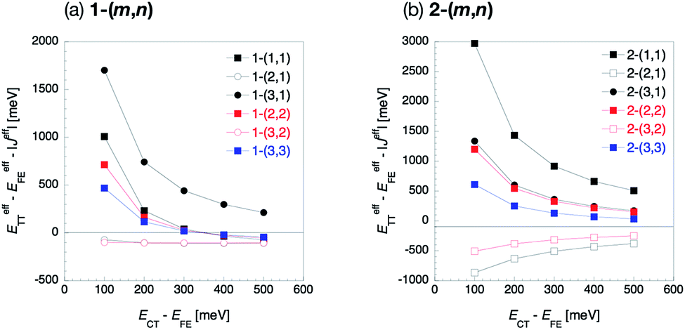 | ||
| Fig. 7 CT state energy dependence of the effective energy difference defined by eqn (16) of 1-(m, n) (a) and 2-(m, n) (b). Filled and blank markers represent even and odd combinations, respectively. Black, red and blue markers represent n = 1, 2 and 3, respectively. Square and circle markers represent m = n and m ≠ n, respectively. | ||
5.5 Relationship with single-molecular devices and intramolecular electron or hole transfer systems
We note here the relationships between the above discussion and the previous studies of quantum interference in single-molecular conductors and intramolecular electron transfer systems, where the quantum interference effect has also been studied.67–69 In the research area of single-molecular devices, quantum interference is well recognized and considered as one of the most important issues. In the previous discussions of quantum interference in that field, the phase relationship between a bridge and electrodes, which corresponds to chromophores in this study, do not play any roles in charge conductivity because the electrodes have a continuum state, where we cannot know the phase of wavefunction. The phase effect of an electrode would be averaged and thus be hidden by the dense continuum state, so that the relative sign of couplings provided through each bridge would not affect the total transmission (coupling). However, the relative phase of chromophore MOs at the bridge-linked positions is crucial for SF and TTA, as shown in the comparison between (I-PP) and (II-PP), and between (I-PN) and (II-PN). Due to the discrete energy levels of the HOMO and LUMO of chromophores, we have found crucial roles of the relative phase of the MOs at the bridge-linked positions.On the other hand, intramolecular electron or hole transfer systems such as norbornyldienes were investigated in terms of electronic coupling through covalent bonds.67,68 Many kinds of bridges with different length and connection patterns were considered, and their effects on the electron or hole transfer rate from the quantum interference viewpoint were discussed. Unlike these series of studies, where one of the horizontal couplings is the issue, SF and TTA need an additional consideration of the other electronic coupling, that is, the non-horizontal coupling, whose relative value to the horizontal one was shown to be crucial to tune the energetic conditions. Consequently, we have found many interesting quantum interference effects in the four cases (I-PP), (I-PN), (II-PP) and (II-PN) on the FE–TT state energetics, which are not observed in the fields of single-molecular conductors nor intramolecular electron (hole) transfer systems.
6 Conclusions
We have investigated the tetracene dimers bridged through two polyynes with various lengths and two bridging patterns as examples of doubly-bridged intramolecular SF and/or TTA systems by density functional theory calculations combined with Green's function method. In order to achieve the desired energetic conditions for SF and/or TTA, we have proposed the idea of quantum interference within a bridge and between bridges both in mathematical and graphical representations. We have discussed the four situations of bridging manners, that is, the cases (I-PP), (I-PN), (II-PP) and (II-PN). The case (I-PP) induces large bridge-mediated contributions in all the Fock matrix elements, while the case (I-PN) induces small bridge-mediated contributions in all the Fock matrix elements. The case (II-PP) induces large horizontal couplings and small non-horizontal couplings, while the case (II-PN) induces small horizontal couplings and large non-horizontal couplings. These four cases are classified by which the PC or NC bridges are used as well as by the bridge-linked positions. As the horizontal and non-horizontal couplings are related to the stabilization in the FE and TT states, respectively, as shown in the perturbation analysis, these element-selective design guidelines of the coupling matrix elements would realize the relative energy tuning for SF or TTA using the same target materials.Indeed, we have achieved the desired energetic conditions for SF in the cases (I-PN) and (II-PN), and for TTA in the cases (I-PP) and (II-PP) using the common chromophore, tetracene. We have analysed the differences of them through the perturbation approach. In the perturbation analysis, we have found that in the case (I-PP) the lowest state is the FE or TT state (CT energy sensitive), in the case (I-PN) the TT state, in the case (II-PP) the FE state and in the case (II-PN) the TT state. In spite of the same lowest state in the cases (I-PN) and (II-PN), we have also found the exothermicity in SF is larger in the case (II-PN) than (I-PN). We have also shown the inequality eqn (16), which represents the importance of the element-selective design of electronic couplings especially for realizing efficient SF in near isothermic chromophores such as tetracene. Comparisons with the previous reports on tetracene dimers indicate the validity of our designed molecules and design strategies for fast and high-yield SF. We have also found that the quantum interference between bridges proposed here is crucial in covalently-linked SF and TTA systems in contrast to single molecular conductors and intramolecular electron/hole transfer systems. The proposed strategy for realizing the desired patterns of the electronic couplings in a covalently-linked system is not limited to polyynes but can be applied to many other bridge moieties. Relative MO phases can be easily obtained by conventional ab initio calculations or even by considering a simple orbital diagram derived from, for example, Hückel approximation level of theory.
Acknowledgements
This work is supported by JSPS KAKENHI Grant Number JPA2645050 in JSPS Research Fellowship for Young Scientists, Grant Number JP25248007 in Scientific Research (A), Grant Number JP24109002 in Scientific Research on Innovative Areas “Stimuli-Responsive Chemical Species”, Grant Numbers JP15H00999 and 17H05157 in Scientific Research on Innovative Areas “π-System Figuration”, and Grant Number JP26107004 in Scientific Research on Innovative Areas “Photosynergetics”. This is also partly supported by King Khalid University through a grant RCAMS/KKU/001-16 under the Research Center for Advanced Materials Science at King Khalid University, Kingdom of Saudi Arabia.References
- M. B. Smith and J. Michl, Chem. Rev., 2010, 110, 6891–6936 CrossRef CAS PubMed.
- M. B. Smith and J. Michl, Annu. Rev. Phys. Chem., 2013, 64, 361–386 CrossRef CAS PubMed.
- T. N. Singh-Rachford and F. N. Castellano, Coord. Chem. Rev., 2010, 254, 2560–2573 CrossRef CAS.
- J. Zhou, Q. Liu, W. Feng, Y. Sun and F. Li, Chem. Rev., 2015, 115, 395–465 CrossRef CAS PubMed.
- T. Minami and M. Nakano, J. Phys. Chem. Lett., 2012, 3, 145–150 CrossRef CAS.
- T. Minami, S. Ito and M. Nakano, J. Phys. Chem. Lett., 2012, 3, 2719–2723 CrossRef CAS PubMed.
- T. Minami, S. Ito and M. Nakano, J. Phys. Chem. Lett., 2013, 4, 2133–2137 CrossRef CAS.
- S. Ito, T. Minami and M. Nakano, J. Phys. Chem. C, 2012, 116, 19729–19736 CAS.
- S. Ito and M. Nakano, J. Phys. Chem. C, 2015, 119, 148–157 CAS.
- S. Ito, T. Nagami and M. Nakano, J. Phys. Chem. Lett., 2016, 7, 3925–3930 CrossRef CAS PubMed.
- T. Zeng and N. Ananth, J. Am. Chem. Soc., 2014, 136, 12638–12647 CrossRef CAS PubMed.
- A. Akdag, Z. Havlas and J. Michl, J. Am. Chem. Soc., 2012, 134, 14624–14631 CrossRef CAS PubMed.
- W. M. Moller and M. Pope, J. Chem. Phys., 1973, 59, 2760–2761 CrossRef CAS.
- H. Bouchriha, V. Ern, J. L. L. Fave, C. Guthmann and M. Schott, J. Phys., 1978, 39, 257–271 CAS.
- G. B. Piland and C. J. Bardeen, J. Phys. Chem. Lett., 2015, 6, 1841–1846 CrossRef CAS PubMed.
- M. W. B. Wilson, A. Rao, K. Johnson, S. Gélinas, R. Di Pietro, J. Clark and R. H. Friend, J. Am. Chem. Soc., 2013, 135, 16680–16688 CrossRef CAS PubMed.
- H. L. Stern, A. J. Musser, S. Gelinas, P. Parkinson, L. M. Herz, M. J. Bruzek, J. Anthony, R. H. Friend and B. J. Walker, Proc. Natl. Acad. Sci. U. S. A., 2015, 201503471 Search PubMed.
- W.-L. Chan, M. Ligges and X.-Y. Zhu, Nat. Chem., 2012, 4, 840–845 CrossRef CAS PubMed.
- S. R. Yost, J. Lee, M. W. B. Wilson, T. Wu, D. P. McMahon, R. R. Parkhurst, N. J. Thompson, D. N. Congreve, A. Rao, K. Johnson, M. Y. Sfeir, M. G. Bawendi, T. M. Swager, R. H. Friend, M. a. Baldo and T. Van Voorhis, Nat. Chem., 2014, 6, 492–497 CrossRef CAS PubMed.
- P. M. Zimmerman, F. Bell, D. Casanova and M. Head-Gordon, J. Am. Chem. Soc., 2011, 133, 19944–19952 CrossRef CAS PubMed.
- P. M. Zimmerman, C. B. Musgrave and M. Head-Gordon, Acc. Chem. Res., 2013, 46, 1339–1347 CrossRef CAS PubMed.
- D. Casanova, J. Chem. Theory Comput., 2014, 10, 324–334 CrossRef CAS PubMed.
- X. Feng, A. V. Luzanov and A. I. Krylov, J. Phys. Chem. Lett., 2013, 4, 3845–3852 CrossRef CAS.
- S. M. Parker and T. Shiozaki, J. Chem. Theory Comput., 2014, 10, 3738–3744 CrossRef CAS PubMed.
- K. Aryanpour, A. Shukla and S. Mazumdar, J. Phys. Chem. C, 2015, 119, 6966–6979 Search PubMed.
- S. M. Parker, T. Seideman, M. A. Ratner and T. Shiozaki, J. Phys. Chem. C, 2014, 118, 12700–12705 CAS.
- B. J. Walker, A. J. Musser, D. Beljonne and R. H. Friend, Nat. Chem., 2013, 5, 1019–1024 CrossRef CAS PubMed.
- M. W. B. Wilson, A. Rao, J. Clark, R. S. S. Kumar, D. Brida, G. Cerullo and R. H. Friend, J. Am. Chem. Soc., 2011, 133, 11830–11833 CrossRef CAS PubMed.
- A. A. Bakulin, S. E. Morgan, T. B. Kehoe, M. W. B. Wilson, A. W. Chin, D. Zigmantas, D. Egorova and A. Rao, Nat. Chem., 2016, 8, 16–23 CrossRef CAS PubMed.
- A. J. Musser, M. Liebel, C. Schnedermann, T. Wende, T. B. Kehoe, A. Rao and P. Kukura, Nat. Phys., 2015, 11, 352–357 CrossRef CAS.
- L. Wang, Y. Olivier, O. V. Prezhdo and D. Beljonne, J. Phys. Chem. Lett., 2014, 5, 3345–3353 CrossRef CAS PubMed.
- T. C. Berkelbach, M. S. Hybertsen and D. R. Reichman, J. Chem. Phys., 2013, 138, 114103 CrossRef PubMed.
- T. C. Berkelbach, M. S. Hybertsen and D. R. Reichman, J. Chem. Phys., 2014, 141, 074705 CrossRef PubMed.
- J. Li, Z. Chen, Q. Zhang, Z. Xiong and Y. Zhang, Org. Electron., 2015, 26, 213–217 CrossRef CAS.
- G. B. Piland, J. J. Burdett, D. Kurunthu and C. J. Bardeen, J. Phys. Chem. C, 2013, 117, 1224–1236 CAS.
- S. T. Roberts, R. E. McAnally, J. N. Mastron, D. H. Webber, M. T. Whited, R. L. Brutchey, M. E. Thompson and S. E. Bradforth, J. Am. Chem. Soc., 2012, 134, 6388–6400 CrossRef CAS PubMed.
- J. Herz, T. Buckup, F. Paulus, J. U. Engelhart, U. H. F. Bunz and M. Motzkus, J. Phys. Chem. A, 2015, 119, 6602–6610 CrossRef CAS PubMed.
- S. Amemori, Y. Sasaki, N. Yanai and N. Kimizuka, J. Am. Chem. Soc., 2016, 138, 8702–8705 CrossRef CAS PubMed.
- P. Duan, N. Yanai, H. Nagatomi and N. Kimizuka, J. Am. Chem. Soc., 2015, 137, 1887–1894 CrossRef CAS PubMed.
- D. Kato, H. Sakai, N. V. Tkachenko and T. Hasobe, Angew. Chem., Int. Ed., 2016, 55, 5230–5234 CrossRef CAS PubMed.
- A. M. Müller, Y. S. Avlasevich, K. Müllen and C. J. Bardeen, Chem. Phys. Lett., 2006, 421, 518–522 CrossRef.
- A. M. Müller, Y. S. Avlasevich, W. W. Schoeller, K. Müllen and C. J. Bardeen, J. Am. Chem. Soc., 2007, 129, 14240–14250 CrossRef PubMed.
- J. C. Johnson, A. Akdag, M. Zamadar, X. Chen, A. F. Schwerin, I. Paci, M. B. Smith, Z. Havlas, J. R. Miller, M. A. Ratner, A. J. Nozik and J. Michl, J. Phys. Chem. B, 2013, 117, 4680–4695 CrossRef CAS PubMed.
- P. J. Vallett, J. L. Snyder and N. H. Damrauer, J. Phys. Chem. A, 2013, 117, 10824–10838 CrossRef CAS PubMed.
- E. C. Alguire, J. E. Subotnik and N. H. Damrauer, J. Phys. Chem. A, 2015, 119, 299–311 CrossRef CAS PubMed.
- J. D. Cook, T. J. Carey and N. H. Damrauer, J. Phys. Chem. A, 2016, 120, 4473–4481 CrossRef CAS PubMed.
- J. Zirzlmeier, D. Lehnherr, P. B. Coto, E. T. Chernick, R. Casillas, B. S. Basel, M. Thoss, R. R. Tykwinski and D. M. Guldi, Proc. Natl. Acad. Sci. U. S. A., 2015, 112, 5325–5330 CrossRef CAS PubMed.
- J. Zirzlmeier, R. Casillas, S. R. Reddy, P. B. Coto, D. Lehnherr, E. T. Chernick, I. Papadopoulos, M. Thoss, R. R. Tykwinski and D. M. Guldi, Nanoscale, 2016, 8, 10113–10123 RSC.
- N. V. Korovina, S. Das, Z. Nett, X. Feng, J. Joy, R. Haiges, A. I. Krylov, S. E. Bradforth and M. E. Thompson, J. Am. Chem. Soc., 2016, 138, 617–627 CrossRef CAS PubMed.
- X. Feng, D. Casanova and A. I. Krylov, J. Phys. Chem. C, 2016, 120, 19070–19077 CAS.
- E. G. Fuemmeler, S. N. Sanders, A. B. Pun, E. Kumarasamy, T. Zeng, K. Miyata, M. L. Steigerwald, X.-Y. Zhu, M. Y. Sfeir, L. M. Campos and N. Ananth, ACS Cent. Sci., 2016, 2, 316–324 CrossRef CAS PubMed.
- S. Ito, T. Nagami and M. Nakano, J. Phys. Chem. A, 2016, 120, 6236–6241 CrossRef CAS PubMed.
- S. N. Sanders, E. Kumarasamy, A. B. Pun, K. Appavoo, M. L. Steigerwald, L. M. Campos and M. Y. Sfeir, J. Am. Chem. Soc., 2016, 138, 7289–7297 CrossRef CAS PubMed.
- S. N. Sanders, E. Kumarasamy, A. B. Pun, M. T. Trinh, B. Choi, J. Xia, E. J. Taffet, J. Z. Low, J. R. Miller, X. Roy, X. Y. Zhu, M. L. Steigerwald, M. Y. Sfeir and L. M. Campos, J. Am. Chem. Soc., 2015, 137, 8965–8972 CrossRef CAS PubMed.
- S. N. Sanders, E. Kumarasamy, A. B. Pun, M. L. Steigerwald, M. Y. Sfeir and L. M. Campos, Angew. Chem., Int. Ed., 2016, 128, 1–6 CrossRef.
- T. Zeng and P. Goel, J. Phys. Chem. Lett., 2016, 7, 1351–1358 CrossRef CAS PubMed.
- D. Dzebo, K. Börjesson, V. Gray, K. Moth-Poulsen and B. Albinsson, J. Phys. Chem. C, 2016, 120, 23397–23406 CAS.
- S. Ito, T. Nagami and M. Nakano, Phys. Chem. Chem. Phys., 2017, 19, 5737–5745 RSC.
- J. Vura-Weis, M. D. Newton, M. R. Wasielewski and J. E. Subotnik, J. Phys. Chem. C, 2010, 114, 20449–20460 CAS.
- F. C. Spano, Acc. Chem. Res., 2010, 43, 429–439 CrossRef CAS PubMed.
- N. J. Hestand and F. C. Spano, J. Chem. Phys., 2015, 143, 244707 CrossRef PubMed.
- H. Yamagata, C. M. Pochas and F. C. Spano, J. Phys. Chem. B, 2012, 116, 14494–14503 CrossRef CAS PubMed.
- T. Zeng, J. Phys. Chem. Lett., 2016, 4405–4412 CrossRef CAS PubMed.
- R. Tempelaar and D. R. Reichman, J. Chem. Phys., 2017, 146, 174703 CrossRef PubMed.
- P. C. P. de Andrade and J. A. Freire, J. Chem. Phys., 2003, 118, 6733–6740 CrossRef CAS.
- P. C. P. de Andrade and J. A. Freire, J. Chem. Phys., 2004, 120, 7811–7819 CrossRef CAS PubMed.
- M. D. Newton, Chem. Rev., 1991, 91, 767–792 CrossRef CAS.
- K. D. Jordan and M. N. Paddon-Row, Chem. Rev., 1992, 92, 395–410 CrossRef CAS.
- C. J. Lambert, Chem. Soc. Rev., 2015, 44, 875–888 RSC.
- T. Tada and K. Yoshizawa, Phys. Chem. Chem. Phys., 2015, 17, 32099–32110 RSC.
- Y. Tomkiewicz, R. P. Groff and P. Avakian, J. Chem. Phys., 1971, 54, 4504–4507 CrossRef CAS.
- J. Tanaka, Bull. Chem. Soc. Jpn., 1964, 38, 86–103 CrossRef.
- M. Komfort, H. G. Löhmannsröben and T. Salthammer, J. Photochem. Photobiol., A, 1990, 51, 215–227 CrossRef CAS.
- B. Stevens, S. R. Perez and J. A. Ors, J. Am. Chem. Soc., 1974, 96, 6846–6850 CrossRef CAS.
- E. J. Bowen, E. Mikiewicz and F. W. Smith, Proc. Phys. Soc., London, Sect. A, 1949, 62, 26–31 CrossRef.
- K. Tahara and Y. Tobe, Chem. Rev., 2006, 106, 5274–5290 CrossRef CAS PubMed.
- A. Orita and J. Otera, Chem. Rev., 2006, 106, 5387–5412 CrossRef CAS PubMed.
- W. A. Chalifoux and R. R. Tykwinski, C. R. Chim., 2009, 12, 341–358 CrossRef CAS.
- S. Kato, N. Takahashi and Y. Nakamura, J. Org. Chem., 2013, 78, 7658–7663 CrossRef CAS PubMed.
- Y. Tobe, I. Ohki, M. Sonoda, H. Niino, T. Sato and T. Wakabayashi, J. Am. Chem. Soc., 2003, 125, 5614–5615 CrossRef CAS PubMed.
- I. Hisaki, T. Eda, M. Sonoda, H. Niino, T. Sato, T. Wakabayashi and Y. Tobe, J. Org. Chem., 2005, 70, 1853–1864 CrossRef CAS PubMed.
- P. N. W. Baxter, A. Al Ouahabi, J. P. Gisselbrecht, L. Brelot and A. Varnek, J. Org. Chem., 2012, 77, 126–142 CrossRef CAS PubMed.
- J. Antony and S. Grimme, Phys. Chem. Chem. Phys., 2006, 8, 5287–5293 RSC.
- H. Iikura, T. Tsuneda, T. Yanai and K. Hirao, J. Chem. Phys., 2001, 115, 3540–3544 CrossRef CAS.
- C. Lee, W. Yang and R. G. Parr, Phys. Rev. B: Condens. Matter Mater. Phys., 1988, 37, 785–789 CrossRef CAS.
- Y. Tawada, T. Tsuneda, S. Yanagisawa, T. Yanai and K. Hirao, J. Chem. Phys., 2004, 120, 8425–8433 CrossRef CAS PubMed.
- P. C. Hariharan and J. A. Pople, Theor. Chim. Acta, 1973, 28, 213–222 CrossRef CAS.
- M. J. Frisch, G. W. Trucks, H. B. Schlegel, G. E. Scuseria, M. A. Robb, J. R. Cheeseman, G. Scalmani, V. Barone, B. Mennucci, G. A. Petersson, H. Nakatsuji, M. Caricato, X. Li, H. P. Hratchian, A. F. Izmaylov, J. Bloino, G. Zheng, J. L. Sonnenberg, M. Hada, M. Ehara, K. Toyota, R. Fukuda, J. Hasegawa, M. Ishida, T. Nakajima, Y. Honda, O. Kitao, H. Nakai, T. Vreven, J. A. Montgomery Jr, J. E. Peralta, F. Ogliaro, M. Bearpark, J. J. Heyd, E. Brothers, K. N. Kudin, V. N. Staroverov, T. Keith, R. Kobayashi, J. Normand, K. Raghavachari, A. Rendell, J. C. Burant, S. S. Iyengar, J. Tomasi, M. Cossi, N. Rega, J. M. Millam, M. Klene, J. E. Knox, J. B. Cross, V. Bakken, C. Adamo, J. Jaramillo, R. Gomperts, R. E. Stratmann, O. Yazyev, A. J. Austin, R. Cammi, C. Pomelli, J. W. Ochterski, R. L. Martin, K. Morokuma, V. G. Zakrzewski, G. A. Voth, P. Salvador, J. J. Dannenberg, S. Dapprich, A. D. Daniels, Ö. Farkas, J. B. Foresman, J. V. Ortiz, J. Cioslowski and D. J. Fox, Gaussian 09, Revision B.01, Gaussian, Inc., Wallingford CT, 2009 Search PubMed.
- S. Ito, T. Nagami and M. Nakano, J. Phys. Chem. Lett., 2015, 6, 4972–4977 CrossRef CAS PubMed.
- Y. Yao, Phys. Rev. B, 2016, 93, 1–5 CrossRef.
- N. Renaud and F. C. Grozema, J. Phys. Chem. Lett., 2015, 6, 360–365 CrossRef CAS PubMed.
- H. Tamura, M. Huix-Rotllant, I. Burghardt, Y. Olivier and D. Beljonne, Phys. Rev. Lett., 2015, 115, 1–5 CrossRef PubMed.
- Y. Fujihashi and A. Ishizaki, J. Phys. Chem. Lett., 2016, 7, 363–369 CrossRef CAS PubMed.
- M. Nakano, S. Ito, T. Nagami, Y. Kitagawa and T. Kubo, J. Phys. Chem. C, 2016, 120, 22803–22815 CAS.
- E. Clar, Polyaromatic Hydrocarbons, Academic Press, New York, 1964 Search PubMed.
- G. Weiser, L. Sebastian and F. Physikalische, Chem. Phys., 1981, 61, 125–135 CrossRef.
- H. Yamagata, J. Norton, E. Hontz, Y. Olivier, D. Beljonne, J. L. Brédas, R. J. Silbey and F. C. Spano, J. Chem. Phys., 2011, 134, 204703 CrossRef CAS PubMed.
- L. Berstis and K. K. Baldridge, Phys. Chem. Chem. Phys., 2015, 17, 30842–30853 RSC.
- E. Busby, T. C. Berkelbach, B. Kumar, A. Chernikov, Y. Zhong, H. Hlaing, X.-Y. Zhu, T. F. Heinz, M. S. Hybertsen, M. Y. Sfeir, D. R. Reichman, C. Nuckolls and O. Yaffe, J. Am. Chem. Soc., 2014, 136, 10654–10660 CrossRef CAS PubMed.
Footnote |
| † Electronic supplementary information (ESI) available: Other possible phase patterns for case (I-PP); definition of relative phase of molecular orbital; CT state energy dependence; transition density in tetracene; decomposition analysis of electronic coupling for BET-B; proof of eqn (16); eigenvalues and eigenvectors of Hamiltonian eqn (1): detailed decomposition analysis of 1-(1,1). See DOI: 10.1039/c7ra06032g |
| This journal is © The Royal Society of Chemistry 2017 |