
 Open Access Article
 This Open Access Article is licensed under a
 Creative Commons Attribution 3.0 Unported Licence
Understanding the colorimetric properties of quinoxaline-based pi-conjugated copolymers by tuning their acceptor strength: a joint theoretical and experimental approach†
Sébastien Fagour,
Damien Thirion,
Antoine Vacher,
Xavier Sallenave *,
Gjergji Sini,
Pierre-Henri Aubert,
Frédéric Vidal and
Claude Chevrot
*,
Gjergji Sini,
Pierre-Henri Aubert,
Frédéric Vidal and
Claude Chevrot
LPPI, Université de Cergy-Pontoise, France. E-mail: xavier.sallenave@u-cergy.fr
First published on 21st April 2017
Abstract
A series of five new π-conjugated donor–acceptor–donor (DADn) copolymers are presented, combining a common donating unit (substituted propylenedioxythiophene, ProDOT-(OEtHx)) with five diphenyl-quinoxaline based acceptor units bearing substituents of increasing acceptor strength (OMe < H < F < COOMe < CN). The DADn copolymers, namely P3-X (X = OMe, H, F, COOMe, CN), have been studied in solid state by cyclic voltammetry to investigate their electronic properties during n- and p-doping processes and to determine their electrochemical band gap. UV-Vis spectroscopy reveals a dual-band absorption system in which both high energy and low energy band (HEB and LEB) positions and intensities are governed by the acceptor strength. Density functional theory (DFT) computations were performed on D–A–D trimer model compounds in order to understand the experimental results. A colorimetric study in the CIELAB color space revealed that the modulation of the acceptor strength with σ- or π-electron withdrawing/donating groups leads to shades of blue to green upon increasing the acceptor strength. The polymers can also switch to a grey color upon p-doping. Finally, a detailed discussion on color–structure relationship provides valuable insights on molecular design principles to render cyan and green colors.
Introduction
In the past few decades, great attention has been devoted to the development of conjugated polymers for both scientific and industrial applications. Electron-rich heterocyclic-based polymers such as polythiophenes and their derivatives are among the most promising and best studied π-conjugated polymers because of their electronic and optoelectronic properties and the improvement in flexibility through synthetic modifications. These polymers have been used as materials in many areas like organic solar cells (OSC),1 organic light emitting diodes,2 organic field effect transistors3 and electrochromic displays.4 Especially in the field of electrochromic (EC) displays, thiophene-based cathodically coloring EC-polymers have demonstrated attractive properties.5 Shades of polymers with purple, magenta, red and orange colors in their neutral states and transmissive in the oxidized state have already been reported by the Reynolds group.6,7 The control of these colors is possible using polymers such as open and closed ring dialkoxythiophene and mixes thereof. These colors account for the 1st and 4th quadrant of the CIELAB plot. Inside the 2nd quadrant, yellow shades can be obtained from higher bandgap polymers. The 3rd quadrant contains shades of blue to green which can only be accessed with a spectrum that shows two absorption bands. In the case of π-conjugated polymers, the structures yielding this last type of spectra are generally of the donor–acceptor (D–A) type.8–11 Throughout the literature a large variety of D–A copolymers have been reported as having a two-band absorption profile. However, despite this variety, only a very limited number of polymers can meet the necessary requirements for a well-shaped spectrum fitted for EC applications. Indeed most of these systems have been developed for OSC, with the pursuit of widely absorbing compounds over the entire visible spectrum (360–740 nm).12,13 In contrast to these properties, EC polymers yield the best colors when they display an absorbance peak with a large differential intensity between the maximum and minimum.In the purpose of electrochromic polymers with blue cyan and green colors, two strategies for band gap control in donor–acceptor copolymers can be identified in the literature. The first method consists in modifying the donor fragments by changing either the nature of the aromatic ring9 or the number of donor units used.14,15 In the second method, the acceptor part can be modified by similar means to those described for the donor part. Several examples of acceptors bonded to thiophene-based donor have been reported: benzothiadiazole,8 benzooxadiazole10 and quinoxaline derivatives.9 The modification of the acceptor groups can also be done either by chemical modification of benzothiadiazole16 or using functionalized quinoxalines.17–19 The use of acceptors based on diphenyl-quinoxaline which possesses two distinct phenyl rings is one of the widely investigated units because of its easy synthesis and versatility.12,20
In this work, we report an attempt to control the color of donor–acceptor conjugated polymers by inducing modifications to the acceptor part of the system. The polymers were synthesized by associating two electron-rich propylenedioxythiophene units (ProDOT(OEtHex)2) namely 3,3-bis(((2-ethylhexyl)oxy)methyl)-3,4-dihydro-2H-thieno[3,4-b][1,4]dioxepine (donor D) with different substituted aryl-quinoxaline units (acceptor A) namely 2,3-bis-(p-subst-phenyl)-2,3-quinoxalines in a D–A–Dn structure (Scheme 1). Moreover, the donor unit is bearing two ethylhexyl chains giving the polymers both a good solubility and processability in common organic solvents.6 Finally, substituting the phenyl units borne by the quinoxaline with functional groups possessing different electron-donor and electron-acceptor properties allows a fine tuning of the overall acceptor strength of the quinoxaline moiety. This kind of control through quinoxaline derivatives have already been described in organic solar cells,12,21,22 and in electrochromic cells, but on a limited range of substituents.19,23 Considering a non-substituted diphenyl-quinoxaline (DPQ) based polymer P3-H (Scheme 1), we have synthesized four other polymers, reported as P3-OMe, P3-F, P3-COOMe, P3-CN. Molecular modelling in the frame of density functional theory (DFT) was used to study the structures and properties of trimer model corresponding to all the synthesized polymers. Through a thorough discussion of the relationship between structure, energetic levels, and color control in DADn polymer structures, new guidelines for molecular design are proposed.
 | ||
| Scheme 1 Donor and acceptor units – combined monomers and their corresponding polymers. | ||
Experimental
Materials
Commercially available reagents and solvents were purchased from Alfa Aesar or Sigma-Aldrich and were used without further purifications other than those detailed below. Tetrahydrofurane (THF), toluene and dimethylformamide (DMF) were dried by distillation from sodium/benzophenone, sodium and calcium hydride, respectively, and store over 4 Å molecular sieves. Analytical thin layer chromatography was carried out using aluminium backed plates coated (Macherey Nagel) and visualized under UV light (at 254 and 365 nm). Purification by column chromatography were carried out using silica 60A CC 40–63 μm (Macherey-Nagel).Techniques of analysis
1H and 13C NMR spectra were recorded using a Bruker Avance 250 MHz spectrometer. Chemical shifts are given in ppm using the residual solvent signals of CDCl3 (7.26 ppm for the proton and 77.00 ppm for the carbon) as an internal reference. The following abbreviations have been used for the NMR assignment: s for singlet, d for doublet, m for multiplet and br for broad. High resolution mass spectra were recorded at the Small Molecule Mass Spectrometry Platform of IMAGIF. Steric Exclusion Chromatography (SEC) was performed on a Viscotek liquid chromatography system with its internal differential refractive index detector (DRI) at 35 °C and columns at 40 °C. Two waters columns were used with HPLC grade THF as the mobile phase at a flow rate of 1 mL min−1. Injections were made at 2 mg mL−1 sample concentration using a 50 μL injection volume. Retention time was calibrated against narrow molecular weight polystyrene standards (Varian Easivial PS-M).Thermogravimetric analysis (TGA) was carried out under argon flow at a heating rate of 20 °C min−1 to 600 °C using a TA Instruments Q50 analyser. The temperature of thermal degradation (Td2%) was measured at the point of 2% weight loss relative to the weight at room temperature. Electrochemical measurements were performed on a potentiosat/galvanostat (VMP, Biologic-SA). A single cell three-electrode configuration was used for all experiments with platinum disk (2 mm diameter) or ITO (Solems, 30 ohm sq−1) as working electrode, platinum grid as counter-electrode and a silver wire as pseudo-reference calibrated vs. ferrocene. UV-Visible spectra were recorded on a Jasco UV/Vis/NIR spectrophotometer in transmission mode (340–760 nm, 1000 nm min−1). Colorimetric data were obtained with a CM-6000 spectrocolorimeter (Konika Minolta). Illuminant C and a 2° observer were used.
Computational methods
In this study trimer model compounds were considered by replacing the ethylhexyl groups by methyl ones. The ethylhexyl chains enhance the solubility of the polymers, but from a computational point of view, they have a relatively low impact on the structure optimization. The calculations were performed in “gas phase” using Density Functional Theory (DFT)24 with the B3LYP25,26 functional. The 6-31G(d,p) basis set was used for all atoms. During the geometry optimizations of the trimer models, constraints on the dihedral angles of the aromatic rings were introduced to get closer to the minimal energy of the system and avoid local minima. Lifting the constraints in a subsequent step yielded the optimized structures. The absorption spectra of the model compounds were obtained by means of TD-DFT27–30 calculations at the B3LYP/6-31G(d,p) level in “gas phase”. Gaussian09 (ref. 31) suit of programs was used for all the calculations.Synthesis
The synthetic path was given in Scheme 2. The syntheses of most of 4,4′-di-subst-benzyl 2-X have been reported in the literature previously,32,33 often they are commercially available or intermediates for other compounds. Only 4,4′-dicyanobenzyl (2-CN) was an original derivative and its synthesis is described below. | ||
| Scheme 2 Synthesis of quinoxaline polymers from benzothiadiazole based DAD monomers. | ||
Monomer 3-X (0.1 g) was dissolved in chloroform (8 mL). FeCl3 (5 eq.) in nitromethane (1 mL) was added dropwise over 20 minutes. The reaction was stirred for 60 h at room temperature. The solution was then poured into methanol (200 mL). The precipitate was collected by filtration, washed once by methanol and dissolved in chloroform (120 mL). Hydrazine monohydrate (2 mL) was added and the solution was stirred for 4 h at room temperature. After evaporation, the concentrate was precipitated into methanol (200 mL). The precipitate was filtered and purified by Soxhlet extraction with methanol, ethyl acetate and chloroform. The yields and colors are summarized in Table 1. Molecular weights were further investigated via polystyrene calibrated SEC with THF as the mobile phase. As illustrated in Table 1, polymers with number-average molecular weight (Mn) ranging from 13![[thin space (1/6-em)]](https://www.rsc.org/images/entities/char_2009.gif) 500 to 76400 g mol−1 with narrow polydispersity (PDIs) (1.7–3.1) were estimated. Thermogravimetric analysis of the polymers (Table 1) in a nitrogen atmosphere revealed that they all have 2% weight loss values (Td2%) between 255 and 325 °C, demonstrating their high thermal stability.
500 to 76400 g mol−1 with narrow polydispersity (PDIs) (1.7–3.1) were estimated. Thermogravimetric analysis of the polymers (Table 1) in a nitrogen atmosphere revealed that they all have 2% weight loss values (Td2%) between 255 and 325 °C, demonstrating their high thermal stability.
| Polymers | Yield (%) | Color | Mn (g mol−1) | PDI | Td2% (°C) |
|---|---|---|---|---|---|
| P3-OMe | 75 | Dark blue | 13500 |
1.9 | 322 |
| P3-H | 73 | Dark blue | 51400 |
2.8 | 256 |
| P3-F | 78 | Dark blue | 29200 |
2.3 | 305 |
| P3-COOMe | 69 | Dark green | 38400 |
1.7 | 265 |
| P3-CN | 72 | Dark green | 76400 |
3.1 | 276 |
Results and discussion
Energy diagram of the model compounds
The model compounds corresponding to P3-OMe, P3-H, P3-F, P3-COOMe and P3-CN will be reported as trim3-OMe, trim3-H, trim3-F, trim3-COOMe and trim3-CN respectively. The contour plots of different molecular orbitals (MO) corresponding to the unsubstituted trimer model compound trim3-H are given in Fig. 1. Despite the presence of some contribution from the acceptor part, the HOMO of the non-substituted model compound trim3-H is mainly concentrated on the two ProDOT donor units. LUMO presents less mixing, being located mainly on the acceptor part.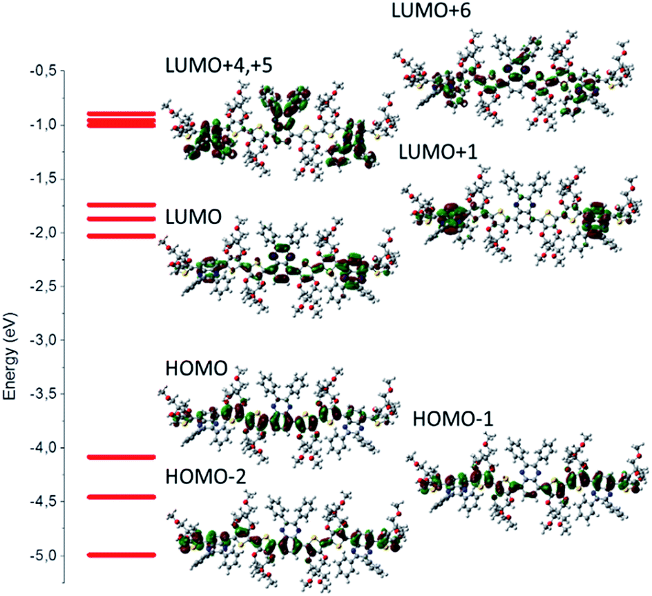 | ||
| Fig. 1 Electronic levels and corresponding contour plots for a selected set of occupied and virtual molecular orbitals for trim 3-H (B3LYP/6-31G(d,p) level in “gas phase”). Note the dominant contribution of the donor moieties on the HOMO distribution (mainly four donor units and one acceptor unit), whereas LUMO is practically localized on the acceptor units with negligible contribution from the donor ones. | ||
Similar comments apply to the substituted model compounds (Fig. S1†). Comparison across the series of model compounds trim3-X (X = OMe, H, F, COOMe, CN) indicates similar degree of donor–acceptor mixing in the HOMOs, whereas less mixing can be observed in the LUMOs for trim3-COOMe, trim3-CN as compared to trim3-OMe, trim3-H, and trim3-F. The higher virtual orbitals seem even more localized on the acceptor units. The contribution of the substituents on the higher virtual orbitals is found to increase as their σ- or π-acceptor/donor strength increases, and becomes visible starting from LUMO+3 (trim3-H) or LUMO+4 (trim3-OMe, trim3-F, trim3-COOMe, trim3-CN). The evolution of a selected set of energy levels corresponding to model compounds are shown in Fig. 2, whereas the numerical results for HOMO and LUMO energies are given in Table 2. The decreasing HOMO energies from trim3-H to trim3-CN in the order H < F < COOMe < CN are consistent with the increasing donor–donor dihedral angles ΦDD (Table S1, Fig. S2†) and with the increasing acceptor strength of the substituents. However, in view of the small contribution of the quinoxaline ring in the HOMO, the influence of the electronegativity-factor in the HOMO energy can be supposed to be of minor importance. The higher HOMO level of trim3-OMe as compared to trim3-H is the consequence of the π-donor effect of the methoxy groups. Compared to HOMOs, the LUMO energies are more sensitive to the nature of the substituent, due to their almost exclusive localization on the quinoxaline ring. This difference is reflected in a larger variation of the LUMO energies as compared to the HOMOs ones (0.72 eV and 0.58 eV respectively). Therefore, a decreasing HOMO–LUMO gap across the series is obtained, with a variation of 0.14 eV between trim3-OMe and trim3-CN.
 | ||
| Fig. 2 Evolution of the HOMO−4 to LUMO+6 energy levels corresponding to trim3-OMe, trim3-H, trim3-F, trim3-COOMe, trim3-CN model compounds. The nature of the virtual orbitals is also indicated. | ||
| Experimental | Theoretical (trimer) | |||||||
|---|---|---|---|---|---|---|---|---|
| Eoxonseta (V) | Eredonseta (V) | IPssb (eV) | EAssb (eV) | ΔEelecc (eV) | EHOMO (eV) | ELUMO (eV) | Eg (eV) | |
| a Referenced vs. ferrocene.b Calculated from IPSS = Eoxonset + 4.8 and EASS = Eredonset + 4.8. Eoxonset and Eredonset are the onset potentials of oxidation and reduction relative to ferrocene redox potential used as calibration reference,22 respectively, taken at the intersection of the two tangents drawn at the rising current and baseline charging current of the CV traces.c ΔEelec is the (electrochemical) band gap of the polymer calculated as ΔEelec = |IPSS − EASS| from redox data. | ||||||||
| P3-OMe | 0.29 | −1.58 | 5.09 | 3.22 | 1.87 | −3.96 | −1.89 | 2.07 |
| P3-H | 0.26 | −1.50 | 5.06 | 3.30 | 1.76 | −4.08 | −2.03 | 2.05 |
| P3-F | 0.39 | −1.53 | 5.19 | 3.27 | 1.92 | −4.21 | −2.16 | 2.05 |
| P3-COOMe | 0.28 | −1.46 | 5.08 | 3.34 | 1.74 | −4.22 | −2.25 | 1.98 |
| P3-CN | 0.25 | −1.38 | 5.05 | 3.42 | 1.63 | −4.54 | −2.61 | 1.93 |
The energy evolution of the virtual orbitals of trimer models (Fig. 2) exhibits interesting differences between compounds trim3-OMe, trim3-H, trim3-F on the one hand and trim3-COOMe, trim3-CN on the other hand. Indeed, two groups of virtual orbitals can be observed in all cases. The lowest group contains LUMO through LUMO+2, exhibiting dominant contribution from the quinoxaline ring (Fig. S1†). The highest group contains LUMO+3 through LUMO+6 and is due to phenyl- or mixed quinoxaline-phenyl contribution.
While the gap between these two groups remains large in the case of trim3-H, trim3-OMe, trim3-F, it is strongly reduced in the case of trim3-COOMe and trim3-CN. We suggest this last effect to be due to the important stabilization of the local-phenyl LUMOs in the presence of –COOMe and –CN substituents, therefore resulting in their efficient mixing with the quinoxaline local LUMOs.
Electrochemical behaviour
The electrochemical properties of the polymers were determined from thin films of each polymer drop coated on platinum electrode. The Fig. 3 presents the cyclic voltamograms (CV) performed in 0.1 mol L−1 TEABF4 in acetonitrile of the different polymers. For π-conjugated polymers, reversibility of doping process depends mainly on the stabilization of the charge carriers (positive or negative polarons/bipolarons)34 by its counter balancing ion and the energy level of the corresponding MO involved in the charge transfer. Upon anodic polarization (0 V to 0.9 V vs. ferrocene), all polymers present a reversible oxidation process starting at around 0.3 V. Corresponding data are summarized in Table 2. The onset potential remains almost unchanged across the series because all polymers exhibit similar donating unit. Also looking at Fig. 1, the contour plot of the HOMO (and HOMO−1) are mainly located on a common DD-Qx-DD extended pi-conjugated system (DD being bis-prodot unit and Qx being quinoxaline one). For that reason, the onset oxidation potential is nearly unchanged. In the cathodic region (0 V to −2.5 V), the n-doping of the polymers is more structure-dependent. The reduction takes place around −1.5 V and does not appear reversible for any of the compounds. The position of the cathodic wave slightly shifts toward less negative potentials following the decreasing acceptor strength of the substituent in the order CN > COOMe > F > H > OMe. In the full region [−2.5 V; −1.0 V] P3-OMe, P3-H and P3-F only present a single charge transfer system while P3-COOMe and P3-CN present consecutive charge transfers. The behaviour is in accordance with energy evolution of the virtual orbitals of computed series of trimer trim3-X. The onset potentials of oxidation and reduction (Eoxonset and Eredonset respectively) of the polymers in their solid state (ss) are directly correlated to their ionization potential (IPSS) and electron affinity (EASS) according to the empirical relationship including experimental electrochemical measurements (IPSS = Eoxonset + 4.8 and EASS = Eredonset + 4.8).35 According to Koopmans theorem,36 the trend in the IPSS (and EASS) values should correlate with that of HOMO (and LUMO) energies across the series. However, the continuous decrease of HOMO energies from trim3-OMe to trim3-CN model compounds (Fig. 2 and Table 2) does not well correlate with the experimental IPSS evolution. While a possible explanation for this discrepancy is discussed in the ESI,† the pertinent information to retain is that IPSS, EASS and the theoretical HOMO–LUMO gaps globally decrease across the series, which basically is due to the stronger sensibility of the LUMO than HOMO energies with respect to the acceptor strength of the substituent. In the cathodic region (Fig. 3), below −1.7 V, additional reduction processes are observed for P3-COOMe and P3-CN. According to the trend observed on Fig. 2, these electrochemical waves are directly correlated to the merging of the two groups of virtual orbitals observed for P3-COOMe and P3-CN.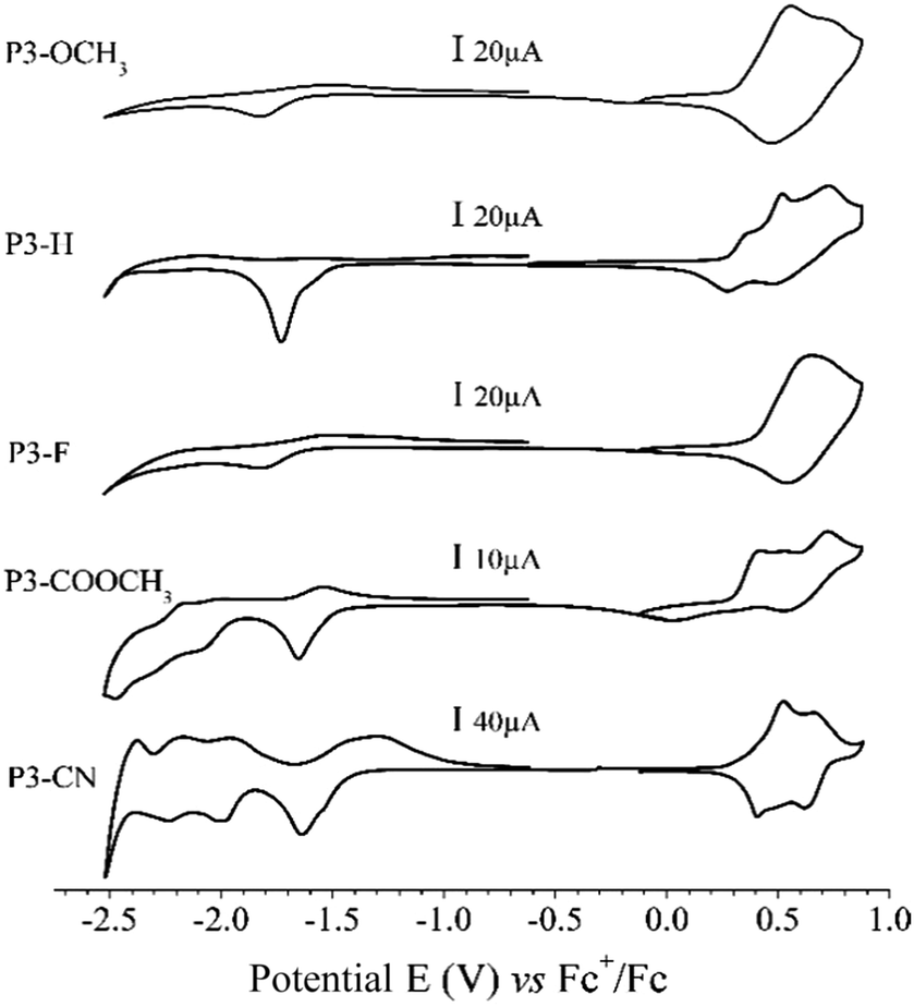 | ||
| Fig. 3 Cyclic Voltamograms (CVs) of polymers P3-X drop cast onto platinum from toluene solutions. Scan rate 10 mV s−1, 0.1 mol L−1 ACN/TEABF4 – all potentials are referenced to ferrocene in 0.1 mol L−1 ACN/TEABF4. | ||
Optical, spectroelectrochemical and electrochromic properties of polymers
The UV-Vis absorption spectra of the five polymers P3-X in solid state are shown in Fig. 4, whereas the numerical results are summarized in Table 3. As expected, all polymers present two major absorption bands in the visible region, which will be designated hereafter as the high-energy and low-energy band (HEB and LEB, respectively). The analysis of the absorption spectra reveals two important trends: (i) with the increasing acceptor strength (OMe < H < F < COOMe < CN), both HEB and LEB bands exhibit a red-shift of their maxima (28 nm and 78 nm respectively, corresponding to 0.21 eV in each case). Except for P3-F, both the red shift and trend in the band gaps are in agreement with the decrease of the electrochemical gap along the series. (ii) The intensity of the HEB globally increases with the increasing acceptor strength CN ≈ COOMe > F > H (apart from of P3-OMe, exhibiting the highest absorption). | ||
| Fig. 4 Absorption spectra of the polymers spray cast on ITO/glass normalized to the low energy band (LEB). Blue: P3-OMe, red: P3-H, black: P3-F, green: P3-COOMe and magenta: P3-CN. | ||
| Polymers | λmax (nm) thin film | Optical gap Eg (eV) | |
|---|---|---|---|
| HEB | LEB | ||
| P3-OMe | 396 | 594 | 1.76 |
| P3-H | 410 | 627 | 1.72 |
| P3-F | 406 | 627 | 1.69 |
| P3-COOMe | 413 | 642 | 1.67 |
| P3-CN | 424 | 672 | 1.60 |
Spectroelectrochemical studies of the polymers were used to examine the evolution of the optical properties as a function of the applied potential. Absorption spectra for all the polymers show that both the LEB and HEB bleach upon oxidation yielding a greyish colour on the electrode (see Fig. 5).
 | ||
| Fig. 5 Spectroelectrochemistry of the polymers on ITO electrode in LiTFSI/ACN (0.1 mol L−1) from their coloured state (neutral form) to bleached state (oxidized form). Applied potential are given vs. Ag pseudo-reference. | ||
The spectroscopic data obtained from the electrochemical switching of the polymers were analysed further to calculate the colorimetric data in the CIELAB colour space. The colorimetric variations are plotted in Fig. 6 and the colours in the neutral and fully oxidized states are reported in Table 4. Connecting to the earlier analysis of absorption spectra (Fig. 4), we will now discuss the relationship between colour and structure of the polymers.
 | ||
| Fig. 6 Colorimetric data obtained from spectroelectrochemical switching study in CIELAB system (C/2°) (projected on isosurface color at level L* = 70). P3-OMe (blue, plain line), P3-H (dash), P3-F (dots), P3-COOMe (dash dot), P3-CN (short dot). | ||
| Polymers | Colored (neutral) | Transmissive (oxidized) | ||||||
|---|---|---|---|---|---|---|---|---|
| L* | a* | b* | L* | a* | b* | |||
| P3-OMe | 79.4 | 0 | −7.5 | Light blue | 85.3 | −2.3 | 1.5 | Transmissive grey |
| P3-H | 77.1 | −5.8 | −13.8 | Cyan | 90.3 | −1.7 | 0.5 | Transmissive grey |
| P3-F | 77.1 | −6.6 | −12.9 | Cyan | 88.1 | −1.3 | −1.2 | Transmissive grey |
| P3-COOMe | 71.4 | −12.2 | −6.8 | Teal | 83.5 | −1.9 | −1.1 | Transmissive grey |
| P3-CN | 63.8 | −15.2 | −2.7 | Green | 76.3 | −0.7 | −1 | Transmissive grey |
The analysis of the coloured (neutral) state is based on the following points. (i) The blue part of the absorption spectrum lies between 360 and 480 nm, the cyan colour between 480 and 500 nm and the green part of the spectrum between 500 and 550 nm. (ii) From a colorimetric point of view, the most important parameter to achieve a vibrant blue to green colour is the dominant wavelength. In the absorption spectra presented in Fig. 5, the dominant wavelength for each compound corresponds to the minimum absorption (MA) between HEB and LEB. The following discussion will show how the colour is tied to both LEB and HEB. (iii) Last important factor in this analysis is that cyan generally results from the equilibrium between the blue and green part of the spectrum. In the case of the non-substituted polymer P3-H, the maxima of the two absorption bands (Fig. 4 and 5) occur at 400 nm (HEB) and 613 nm (LEB). The minimum of the absorption spectra where the blue part of the spectrum is transmitted lies at 450 nm. However, the part of the transmitted light in the case of P3-H spreads from 430 to 536 nm (dashed rectangle in Fig. 5), which leads to a mix between the blue and green part of the spectrum. Consequently, the measured colour in the neutral state is cyan and tends slightly more toward the blue axis (negative b*). The introduction of the fluorine substituent has little effect on the absorption spectrum and despite a slight difference of optical band gap, the position of the LEB remain unchanged. Since the band positions are almost the same, the MA of P3-F is shifted by 2 nm as compared to P3-H and the window of transmitted light is the same for both polymers, resulting in almost identical colour for P3-H and P3-F.
A difference appears upon switching, showing that P3-F has less broad lasso shaped curve than P3-H, its colour hysteresis is then smaller as compared to P3-H (Fig. 6). Compared to P3-H, the methoxy substituted polymer P3-OMe exhibits a hypsochromic shift of both HEB and LEB by 14 and 37 nm respectively. The shift of the LEB filters out more of the green part of the spectrum. The LEB hypsochromic shift added to the absorption of the HEB causes the MA intensity to increase (from 0.15 a.u. for P3-H to 0.25 a.u. for P3-OMe). The blue-green equilibrium of the cyan colour of P3-H is modified to a blue colour. Associated with the low molecular weight of P3-OMe (Table 1), the colour cannot be obtained with much saturation, b* of −7.5 is about the maximum value (Fig. 6). Due to the increased acceptor strength as compared to P3-H, the remaining two polymers P3-COOMe and P3-CN show a bathochromic shift of the MA which lies from 450 to 485 nm for P3-COOMe and from 450 to 500 nm for P3-CN (Fig. 5).
The window of transmitted wavelength is also shifted from 442 to 542 nm for P3-COOMe and from 452 to 544 nm for P3-CN. These wavelengths correspond to a dominant green colour, which is finally obtained for those two polymers (Fig. 6).
Conclusions
We studied a series of conjugated D–A–D copolymers based on ProDOT-(OEtHx) as the donor part and five derivatives of diphenyl-quinoxaline as the acceptor part. The optical spectroscopy reveals a dual-band absorption profile. A colorimetric study revealed that the modulation of the acceptor strength with σ- or π-electron withdrawing/donating groups leads to blue cyan and green colours. Thus, both experimental and DFT results indicate that the chemical modification of the quinoxaline acceptor part of D–A–D polymers can be efficiently used for modulating and fine-tuning the band gap of the polymers and the energy of the HEB and LEB. The variation of these parameters in the case of our compounds leads to shades of blue to green upon increasing the acceptor strength with a possible fine-tuning of the colorimetric and electrochromic properties.Acknowledgements
Our sincere appreciation goes to J.-F. DeCarreau for his insights into colorimetric assessment of materials. We express our thanks to Laurent Bouteiller and Gaelle Pembuong for the SEC analysis of the polymers. This work has benefited from the facilities and expertise of the Small Molecule Mass Spectrometry Platform IMAGIF.Notes and references
- F. Zhang, D. Wu, Y. Xu and X. Feng, J. Mater. Chem., 2011, 21, 17590 RSC.
- J. Pei, W.-L. Yu, W. Huang and A. J. Heeger, Macromolecules, 2000, 33, 2462 CrossRef CAS.
- H. Bronstein, Z. Chen, R. S. Ashraf, W. Zhang, J. Du, J. R. Durrant, P. Shakya Tuladhar, K. Song, S. E. Watkins, Y. Geerts, M. M. Wienk, R. A. J. Janssen, T. Anthopoulos, H. Sirringhaus, M. Heeney and I. McCulloch, J. Am. Chem. Soc., 2011, 133, 3272 CrossRef CAS PubMed.
- R. J. Mortimer, A. L. Dyer and J. R. Reynolds, Displays, 2006, 27, 2 CrossRef CAS.
- P. M. Beaujuge and J. R. Reynolds, Chem. Rev., 2010, 110, 268 CrossRef CAS PubMed.
- B. D. Reeves, C. R. G. Grenier, A. A. Argun, A. Cirpan, T. D. McCarley and J. R. Reynolds, Macromolecules, 2004, 37, 7559 CrossRef CAS.
- A. L. Dyer, M. R. Craig, J. E. Babiarz, K. Kiyak and J. R. Reynolds, Macromolecules, 2010, 43, 4460 CrossRef CAS.
- P. M. Beaujuge, S. V. Vasilyeva, S. Ellinger, T. D. McCarley and J. R. Reynolds, Macromolecules, 2009, 42, 3694 CrossRef CAS.
- S. Tarkuc, Y. A. Udum and L. Toppare, Polymer, 2009, 50, 3458 CrossRef CAS.
- M. İ. Özkut, M. P. Algi, Z. Öztaş, F. Algi, A. M. Önal and A. Cihaner, Macromolecules, 2012, 45, 729 CrossRef.
- G. Sonmez, C. K. F. Shen, Y. Rubin and F. Wudl, Angew. Chem., 2004, 43, 1498 CrossRef CAS PubMed.
- E. Wang, L. Hou, Z. Wang, S. Hellström, F. Zhang, O. Inganäs and M. R. Andersson, Adv. Mater., 2010, 22, 5240 CrossRef CAS PubMed.
- H. Kim, M. Heo, Y. Jin, J. Kim and J. Y. Shim, Bull. Korean Chem. Soc., 2012, 33, 629 CrossRef.
- P. M. Beaujuge, S. Ellinger and J. R. Reynolds, Adv. Mater., 2008, 20, 2772 CrossRef CAS PubMed.
- P. M. Beaujuge, C. M. Amb and J. R. Reynolds, Acc. Chem. Res., 2010, 43, 1396 CrossRef CAS PubMed.
- G. L. Gibson, T. M. McCormick and D. S. Seferos, J. Am. Chem. Soc., 2011, 134, 539 CrossRef PubMed.
- C. Kitamura, S. Tanaka and Y. Yamashita, Chem. Mater., 1996, 8, 570 CrossRef CAS.
- Y. Huang, M. Zhang, L. Ye, X. Guo, C. C. Han, Y. Li and J. Hou, J. Mater. Chem., 2012, 22, 5700 RSC.
- M. Sendur, A. Balan, D. Baran and L. Toppare, J. Polym. Sci., Part A: Polym. Chem., 2011, 49, 4065 CrossRef CAS.
- Y. Lee, Y. M. Nam and W. H. Jo, J. Mater. Chem., 2011, 21, 8583 RSC.
- H. Qin, L. Li, T. Liang, X. Peng, J. Peng and Y. Cao, J. Polym. Sci., Part A: Polym. Chem., 2013, 51, 1565 CrossRef CAS.
- J.-H. Kim, C. E. Song, W. S. Shin, B. Kim, I.-N. Kang and D.-H. Hwang, J. Polym. Sci., Part A: Polym. Chem., 2015, 53, 1904 CrossRef CAS.
- M. Mahmut, T. Awut, I. Nurulla and M. Mijit, J. Polym. Res., 2014, 21, 1 CAS.
- W. Kohn and L. J. Sham, Phys. Rev., 1965, 140, A1133 CrossRef.
- A. D. Becke, J. Chem. Phys., 1993, 98, 5648 CrossRef CAS.
- Y.-S. Lee and M. Kertesz, J. Chem. Phys., 1988, 88, 2609 CrossRef CAS.
- M. E. Casida, C. Jamorski, K. C. Casida and D. R. Salahub, J. Chem. Phys., 1998, 108, 4439 CrossRef CAS.
- E. K. U. Gross and W. Kohn, Phys. Rev. Lett., 1985, 55, 2850 CrossRef CAS PubMed.
- E. K. U. Gross and W. Kohn, Adv. Quantum Chem., 1990, 21, 255 CrossRef CAS.
- E. Runge and E. K. U. Gross, Phys. Rev. Lett., 1984, 52, 997 CrossRef CAS.
- M. J. Frisch, G. W. Trucks, H. B. Schlegel, G. E. Scuseria, M. A. Robb, J. R. Cheeseman, G. Scalmani, V. Barone, B. Mennucci, G. A. Petersson, H. Nakatsuji, M. Caricato, X. Li, H. P. Hratchian, A. F. Izmaylov, J. Bloino, G. Zheng, J. L. Sonnenberg, M. Hada, M. Ehara, K. Toyota, R. Fukuda, J. Hasegawa, M. Ishida, T. Nakajima, Y. Honda, O. Kitao, H. Nakai, T. Vreven, J. A. Montgomery, J. E. Peralta, F. Ogliaro, M. Bearpark, J. J. Heyd, E. Brothers, K. N. Kudin, V. N. Staroverov, R. Kobayashi, J. Normand, K. Raghavachari, A. Rendell, J. C. Burant, S. S. Iyengar, J. Tomasi, M. Cossi, N. Rega, N. J. Millam, M. Klene, J. E. Knox, J. B. Cross, V. Bakken, C. Adamo, J. Jaramillo, R. Gomperts, R. E. Stratmann, O. Yazyev, A. J. Austin, R. Cammi, C. Pomelli, J. W. Ochterski, R. L. Martin, K. Morokuma, V. G. Zakrzewski, G. A. Voth, P. Salvador, J. J. Dannenberg, S. Dapprich, A. D. Daniels, O. Farkas, J. B. Foresman, J. V. Ortiz, J. Cioslowski and D. J. Fox, Gaussian 09, Revision B.01, Gaussian Inc., Wallingford CT, 2009 Search PubMed.
- M. H. Petersen, S. A. Gevorgyan and F. C. Krebs, Macromolecules, 2008, 41, 8986 CrossRef CAS.
- F. Romanov-Michailidis, C. Besnard and A. Alexakis, Org. Lett., 2012, 14, 4906 CrossRef CAS PubMed.
- L. Zuppiroli, S. Paschen and M. N. Bussac, Synth. Met., 1995, 69, 621 CrossRef CAS.
- J. L. Bredas, R. Silbey, D. S. Boudreaux and R. R. Chance, J. Am. Chem. Soc., 1983, 105, 6555 CrossRef CAS.
- T. Koopmans, Physica, 1934, 1, 104 CrossRef.
Footnote |
| † Electronic supplementary information (ESI) available. See DOI: 10.1039/c7ra02535a |
| This journal is © The Royal Society of Chemistry 2017 |