Interfacial layers at a nanometre scale on iron corroded in carbonated anoxic environments

Abstract

Two tests of iron corrosion in compacted clay and clay slurry were performed for several years. The corrosion systems, and especially the interfacial layer between the metal and the corrosion products, were investigated post mortem by SEM-FEG, μRaman, MET and STXM. An Fe(III) oxide layer systematically developed at a nanometer scale between the metal and an outer layer of carbonates. Its presence could explain the slowing down of the corrosion rate usually observed for these systems. Depending of the compactness of the environment the nature of the interfacial layer is not the same.

---

1. Introduction

The corrosion of mild steel in anoxic and aqueous carbonated media¹ is a major issue in different domains (i.e. the in situ conservation of archaeological iron artefacts,^2,3 oil and gas transport in pipelines^4,5 and geological disposal of high-level radioactive wastes in steel canisters, which has been proposed in several countries^6,7). For example, in France, they plan to confine high-level radioactive wastes in deep geologic sites using an overpack of mild steel inserted in mild steel liners. In some early designs, these steel components were expected to be in contact with clay or anoxic clayey solution, where various corrosion processes are likely to occur.⁸ In clayey media, one of the main questions is linked to the existence or absence of a dense interfacial layer formed between the metal and the corrosion products, in addition to an outer layer consisting of Fe^II carbonates/hydroxycarbonates and to a lesser extent, corrosion products containing silica^9,10. This dense layer may in turn control the kinetics of the corrosion. Recent studies suggest the presence of this layer on mild steel and iron materials corroded in carbonated aqueous media.^11–16 This layer has been detected mainly by using electrochemical and micro-characterisation techniques on laboratory-prepared samples under specific conditions. Because it was relatively thin (<1 μm) and seemed to protect steel from aggressive corrosion, it was assumed to be similar to passive films which formed on mild steel in other environments.^17,18 Recent studies^19,20 on archaeological nails corroded in carbonated environments for several centuries have also shown the presence of an interfacial layer consisting of a mixture of magnetite and maghemite between the steel and the Fe carbonate corrosion products. The thickness of this interfacial layer ranges from about 100 nm to several μm. Isotopic labelling experiments showed that D₂O easily penetrates the porous network of the outer carbonate layer, but does not penetrate the outer surface of this oxide layer, presumably due to its significantly lower porosity compared to the other corrosion products. This is in line with the idea that the kinetics of the corrosion process at the metal surface depends on this interfacial layer, as hypothesized by the authors of previous studies.^14,21

Other studies have indicated that the formation of this interfacial layer depends strongly on the local conditions, especially the pH,^14,20 which depends in turn on the transport processes in the porous network of outer corrosion layers. It is therefore essential to confirm the presence of this layer in carbonated environments representative of the rock hosting the nuclear repository. In that context, the influence of the compactness of these environments on the corrosion processes (i.e. compacted clay or empty spaces around the steel overpack) is also an important factor to consider.

The aim of the present study was to identify and characterize an interfacial layer of this kind by performing two long-term experiments in carbonated anoxic and aqueous clayey media. The two systems under investigation differed mainly in terms of the compactness of the external environment (compacted clay or clay slurry, respectively). Characterisation of sample was performed at the micro- and nanoscales from the two systems, using a step-by-step multi-scale (from micrometric to nanometric) approach.

2. Experimental

2.1. Corrosion experiments

The Arcorr2008 setup. Since the Arcorr2008 setup has been previously described in detail,⁹ it will simply be summarized here. Probes were inserted into a brick from the Callovo-Oxfordian clay formation East of Paris Basin. One of these probes was made by a rod of SON68 glass (the non-radioactive equivalent of French nuclear glass) partly encapsulated in two short Armco iron tubes (pure ferrite; 0.0002 w% C, 0.0009 w% Si, 0.33 w% Mn, 0.019 w% Si, 0.005 w% P, 0.03 w% Cu; balance Fe). Two other probes (one of pure ferrite, one of gold) were inserted in parallel for corrosion monitoring. The clay brick was confined in a nickel insert. The high-pressure cell was linked to an autoclave reservoir filled with a solution having the composition of pore water in equilibrium with clay at 90 °C and a calculated pH of 6.07 determined by imposing a CO₂ pressure of 0.5 bars.^22,23 The redox potential was about −200 mV, quoted against the Standard Hydrogen Electrode (SHE). The composition of the water is shown in Table 1. The setup was vacuum-pumped, saturated with synthetic clay pore water at 90 °C, and reacted at this temperature for two years. At the end of this period, the clay brick was extracted from the high-pressure setup and embedded in epoxy resin, and then the block was cut perpendicularly to the probe axes. The sample analysed here (VFA-2008) corresponds to the interface between the clay and one of the short iron tubes embedding the SON68 glass. Monitoring of the corrosion rate (published elsewhere⁹) showed that after an induction period of one month, at a relatively high corrosion rate (around 90 μm per year), there was a continuous decrease in the corrosion rate, down to 0.3 μm per year after a reaction time of almost 700 days.

Table 1 Composition of the Callovo-Oxfordian water used in the corrosion experiments

PCO2 (bars)	0.5
Eh (mV per SHE)	202
Na^+ (mmol L^−1)	39
K^+ (mmol L^−1)	0.96
Ca^2+ (mmol L^−1)	10
Mg^2+ (mmol L^−1)	2.5
Sr^2+ (mmol L^−1)	0.17
Si (mmol L^−1)	0.84
Cl^− (mmol L^−1)	41
SO4^2− (mmol L^−1)	10
Ctotal (mmol L^−1)	10
Al^3+ (mmol L^−1)	8 × 10^−5
Fetotal (Fe^2+ and Fe^3+, mmol L^−1)	0.05

---

Batx setup. The second sample consisted of a section of an iron probe (a massive Armco iron rod) corroded in an autoclave under the same conditions and setup as above (at 90 °C, under lithostatic pressure and anoxic conditions). However, in the second experiment, the rod was immersed for two years in a clay slurry composed of MX 80 bentonite (3%) and synthetic porewater.

2.2. Sample preparation

To minimize the oxidation of the samples and maintain anoxic conditions, the samples were immediately sealed in an aluminium/polypropylene bag under N₂ (PO₂ < 100 ppm). After each step, the samples were stored and transported in hermetically airtight glass jars under a N₂ atmosphere. All the sample preparation steps were carried out in an anoxic glove box. For micro-Raman (μRaman) spectroscopic analyses, a homemade cell with a 1 mm-thick glass window was used to confine the sample and prevent contact with the air.²⁰

Samples were cut into small pieces to fit into 25 mm resin moulds, and impregnated with resin a polished with abrasive silicon carbide papers (Presi, Mecaprex) and absolute ethanol (Fluka). Diamond pastes with a particle size of 3 and 1 μm were used in the final polishing step with ethanol.

Prior to nanoscale investigations, representative areas of the corrosion interfaces were selected and 80 nm-thick sections were collected using a Dual Beam Focused Ion Beam (FIB) system (FEI Strata 235). With the in situ lift-out technique used, the sample was fixed to a TEM grid inside the Dual beam Instrument without being exposed to the atmosphere.

2.3. Microscale investigations

The morphology of the corrosion interfacial layers was investigated with a Field Electron Gun (FEG) scanning electron microscope (SEM) (JEOL 7001F) with a spatial resolution down to 50 nm. Samples were observed in the backscattered electron (BSE) mode with a 15 kV accelerating voltage and a probe current of about 11 pA. Local elemental compositions were determined by Energy Dispersive X-ray (EDX) analysis using a Silicon Drift Detector (SDD; SGX SENSORTECH Company system) controlled by SAMx microanalysis software, which collects high count rates (about 10⁵ counts per s) with a good spectral resolution (130 eV on Mn K-alpha ray). X-ray mapping was carried out using MaxView imaging software (provided by the company SAMX+), after selecting an energy region of interest (ROI) from the EDX spectra of all the elements of interest. μRaman measurements were performed using an Invia Reflex spectrometer from Renishaw®, equipped with a frequency-doubled Nd:YAG laser emitting at a wavelength of 532 nm and a charge-coupled multichannel matrix (CCD) detector cooled by means of the Peltier effect. A 50× optical LEICA microscope objective was employed to focus the laser beam on the samples to a spot size of less than 2 μm with a spectral resolution of about 1 cm⁻¹ and to collect the scattered light. The wavenumber calibration of the spectrometer was checked periodically using the Raman peak at 520 cm⁻¹ using a silicon crystal as a reference. The laser beam power on the surface of the sample was decreased to 100 μW to prevent the thermal degradation of the corrosion products. The absence of phase transformation under the laser beam was checked, even at this very low power. Solid phases were identified by comparison with reference spectra obtained either from solid reference materials with a known composition or spectra available in the literature. μRaman maps were collected using a motorized microscope stage. The data processing giving qualitative information about the main phase present at each pixel, was conducted using a classical method (the “Signal to Baseline” method) based on the selection of the cumulative signal in a ROI corresponding to a wavenumber range characterizing the main peak in each phase under consideration. The maps obtained gave the intensity of the signals collected in the ROI corrected by a linearly modelled baseline value.²⁴ These data processing procedures were conducted using Wire software (Renishaw).

2.4. Nanoscale investigations

The 80 nm thin films were studied using Transmission Electron Microscopy (TEM) and Scanning Transmission X-ray Microscopy (STXM), as described elsewhere.²⁰ Low-resolution imaging and electron diffraction studies were carried out on a FEI Tecnai F20 electron microscope (with a resolution of about 2.4 Å) equipped with a Super Twin objective lens, a 200 kV field emission gun (FEG) and a scanning image observation device (STEM) with a set of STEM detectors (Bright Field, Annular Dark Field and High Angle Angular Dark Field). The TEM was also equipped with an EDX Si(Li) detector (EDAX R-TEM Sapphire) with a resolution of 129 eV for performing elemental analyses. Sensitive samples were mounted on a cold finger inserted into the microscope chamber. In order to prevent damage to the sample and problems due to the magnetic properties of the iron material, a double tilt cryo-holder (at −170 °C) was used and samples were analysed at an angle of incidence with the beam differing from 0°. In the electron diffraction procedures, an area of the order of 200 nm was selected and the selected area electron diffraction patterns were recorded with a camera length of 150 mm. Bright-field images and electron diffraction patterns were collected using a GATAN Orius 1000 CCD camera (11 Megapixel). Gatan Digital Micrograph software was used to process the data. Background subtraction and radial integration of the 2D electron ring patterns were carried out using macros available in the DiffTool package provided with Digital Micrograph software.²⁵ This software, which was used to control the STEM, also managed the acquisition and quantification of the EDS data.

Scanning Transmission X-ray Microscopy (STXM) experiments were performed at the 10ID-1 beamline of the Canadian Light Source (CLS, Saskatoon), with a focused beam 25 nm in diameter.²⁶ Image sequences (stacks) of Near-Edge X-ray Absorption Fine Structure (NEXAFS) were collected on thin films at the Fe L- and C K-edges. The energy range and resolution of the scans were selected so as to obtain a good compromise between the total acquisition time (each image was collected within about 0.5–1 min, and each stack of 130 to 180 images within 1–2 h) and the resolution required in the spectral ranges containing information (such as the L₂ and L₃ edges in the case of Fe¹⁹ and the resonance peaks at the C K edge²⁷). The measured transmitted signals (I_t) were converted into absorbance values using the incident flux (I₀) measured in the absence of the sample. A set of reference spectra were collected of metallic iron, magnetite (Fe₃O₄), maghemite (γ-Fe₂O₃), siderite (FeCO₃) and chukanovite (Fe₂(OH)₂CO₃), all solid phases previously identified as corrosion products.^20,28 Using the procedure described elsewhere,^28,29 the intensity of the reference spectra was quantified to obtain an absolute linear absorbance scale (i.e., absorbance per unit path length of a pure material with a known density) using the computed elemental response outside the structured near-edge region³⁰ and the density of the material. To obtain quantitative maps from the Fe L-edge stacks, Singular Value Decomposition (SVD) was used, which involved fitting the spectrum at each pixel with a linear combination of the quantitative reference spectra. The component maps were then expressed in terms of the equivalent thickness (nm) of the reference compounds.²⁹ The precision (statistical fluctuations) of the SVD fitting procedure is of the order of a few per cent. The accuracy of the absolute thicknesses of the components was mostly affected by systematic errors due to difference in the elemental composition and/or density of the Fe species in the sample and the reference materials. Note however that the relative magnitude and trends can be expected to be independent of the systematic errors. A multiple linear regression curve fitting procedure was used to determine whether the Fe species signals in a component map included more than 1 component),. The final fit selected was that giving the best χ² value without any negative contribution from the reference spectra or the F-test value. All the data processing was performed using aXis2000.³¹

3. Results and discussion

3.1. The Arcorr2008 setup

The corrosion interface for the Arcorr2008 setup has been studied at the micrometric scale in a previous paper.⁹ The sample under investigation in the present study corresponds to that identified as “VFA-2008” interface in this previous study. The corrosion interface consisted of a “Dense Product Layer” with a thickness of about 40 μm in contact with metallic iron, surrounded by an outer layer composed of a mixture of clay and Fe-containing corrosion products called the “Transformed Medium Layer”. This “Transformed Medium Layer” seemed to be very compact. The “Dense Product Layer” consisted mainly of Fe and O, as shown by EDX (Fig. 1). In addition, Si amounts as high as 18 at% were measured in some places, which suggests that the “Dense Product Layer” was composed of a mixture of Fe silicates (poorly ordered phyllosilicates) and Fe carbonates (siderite (FeCO₃), ankerite ((Fe,Ca,Mg)CO₃) and Fe-silicates). It was unfortunately not possible to obtain any reliable μRaman spectroscopic information about the solid phases present in this Si-containing layer, probably because of fluorescence effects and of the disordered nature of the Fe silicate phases.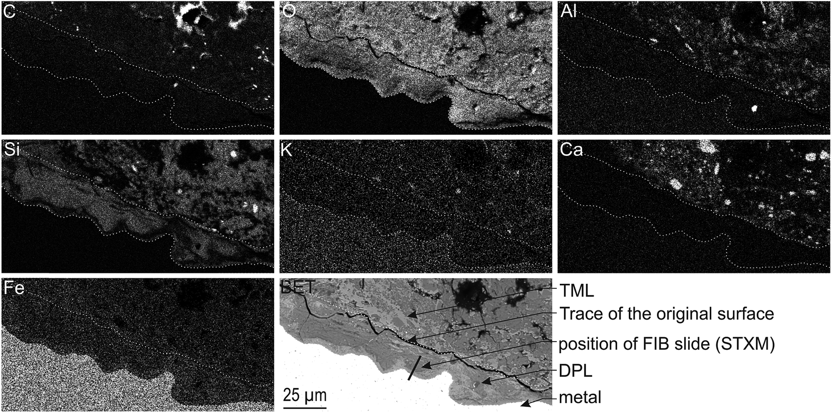

Fig. 1 SEM-BSE image and EDX elemental maps of the Arcorr2008 corrosion interface. The thick segment marks the approximate location of the thin section used in the STXM studies.

A thin film was taken from the sample (Fig. 1) near the metal/“Dense Product Layer” interface, where the Si content was the lowest. A TEM image of this film combined with EDX analysis showed that the main part of the “Dense Product Layer” area had a marbled appearance resulting from the presence of thin fringes of corrosion products containing on average about 5 wt% Si (Fig. 2a and b; point 3). The presence (Fig. 2b point 3) or absence (Fig. 2b point 2) of Si did not really affect the O/Fe ratio, which remained relatively high, close to that of Fe^(II) (hydroxy) carbonates (3 in the case of siderite and 2.5 in that of chukanovite) and higher than expected for magnetite (4/3). Between the main “Dense Product Layer” and the metal, a fringe of variable thickness (up to several tens of nanometres) showed a substantially different contrast from the rest of the corrosion products in the TEM micrograph (Fig. 2a). Local EDS analysis performed in this inner region gave an O/Fe ratio of 1.7 (Fig. 2b number 1), which is substantially lower than in the rest of the “Dense Product Layer”, and closer to the O/Fe ratio of Fe^(II,III) oxides than to that expected for Fe carbonates (such as siderite, ankerite and chukanovite). The nature of this interfacial layer was studied using electron diffraction methods. Only a strong signal from the nearby metallic iron was observed, possibly along with some very weak diffusion rings. This lack of any significant signal may indicate that the interfacial layer has a low crystallinity, but it may also have resulted simply from unfavourable local geometrical conditions for diffraction (such as the presence of an oblique iron-corrosion product interface).

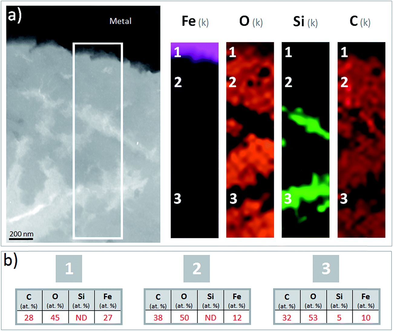Fig. 2 (a) TEM micrograph and EDS-STEM elemental mapping of Fe, O, Si and C and (b) average quantification of point EDS analyses performed at three points on the metal/“Dense Product Layer” interface in the Arcorr2008 sample.

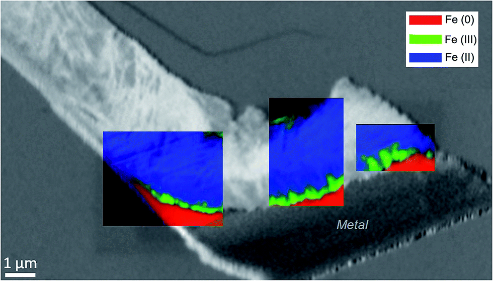
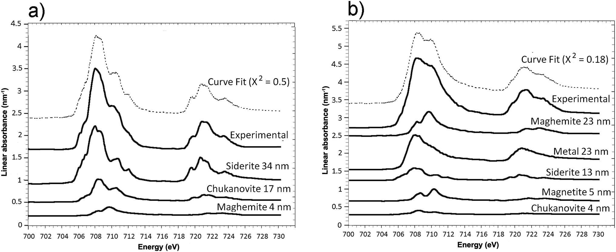
The oxidation state and the molecular environments of selected elements (Fe and C) were mapped at high spatial resolution by STXM.²⁹ First, the distribution of C species was determined by recording absorbance images of the interface at 290 and 280 eV, i.e. at and below the energy of maximum carbonate absorbance, respectively (Fig. 3a). It was then possible to determine the changes in C concentration on a difference map obtained from these two images (Fig. 3b). On this map, the metal, containing no C, shows up in dark grey; in contrast, light grey shades show the presence of carbonate over several μm from the metal/corrosion product interface. Between these two zones, the interfacial area is indicated by a darker grey shade suggesting that C depletion has occurred here in comparison with other corrosion products. To gain information about Fe speciation in these areas, Fe L-edge stacks were collected at various points along the metal/corrosion products interface. Spectral fitting of the Fe L-edge image sequences by SVD was performed using the reference spectra of metallic iron (Fe⁽⁰⁾), siderite (Fe^(II)) and maghemite (Fe^(III)) in order to obtain Fe⁽⁰⁾, Fe^(II) and Fe^(III) component maps (Fig. 4).²⁰ The aim here was to obtain a qualitative picture of the distribution of Fe^(II) and Fe^(III). Several composite color-coded maps of Fe^(II) or Fe^(III) predominance were drawn up at different points on the thin film and superimposed on the C distribution map (Fig. 5). These Fe(III)/Fe(III) maps showed the presence of a thin fringe of several hundred nanometres in thickness at the metal/corrosion product interface (green in Fig. 5), which seems to be more concentrated in Fe^(III) species than the rest of the corrosion products (blue in Fig. 5). The outer boundary of this interfacial fringe, which was not sharply defined, was characterized by a gradual decrease in the Fe^(III) content over a distance of 100–200 nm. On the composite color-coded maps, the darker zones in this layer (blue in Fig. 5) correspond to a weaker measured absorption signal, possibly due to local variations in thickness of the thin film. In order to obtain more detailed information about the Fe species in the various zones, NEXAFS Spectra were extracted (using the threshold masking function provided with Axis 2000 software³²) by averaging all the pixels corresponding to a given zone (consisting of the interfacial fringe or the rest of the corrosion products). The spectrum averaged from the interfacial layer showed two peaks at 708 and 710.2 eV, corresponding to Fe^(II) and Fe^(III) species, respectively (Fig. 6b). In comparison, for the spectra obtained on the outer part of the corrosion product layer (Fig. 6a), the peak at 708 eV was more intense. To gain further quantitative information, curve fitting was performed on the spectra, using metal iron, siderite, chukanovite, magnetite and maghemite as references (Fig. 6). The best fit (χ² = 0.5) with only positive contributions, of the spectrum obtained on the Fe^(II)-rich zone, corresponds to a combination of siderite (35 nm), chukanovite (17 nm), and maghemite (4 nm), thus confirming that Fe^(II) carbonates were the main compounds present in this outer zone (Fig. 6a). In the Fe^(III)-rich interfacial layer, the best fit (χ² = 0.18) was obtained with contributions of maghemite (23 nm), magnetite (5 nm), carbonates (siderite and chukanovite: 17 nm) and iron (23 nm) (Fig. 6b). These STXM analyses clearly show that an interfacial fringe present at the metal-corrosion product interface is mainly composed of solids containing Fe^(III). Fig. 7 shows the proportions of each of these phases, determined over a cross-section extending perpendicular to the metal/oxide interface. The data obtained on the Fe⁽⁰⁾, Fe^(II), Fe^(III) phase mixtures suggest that the interfacial layer was less than 400 nm thick.

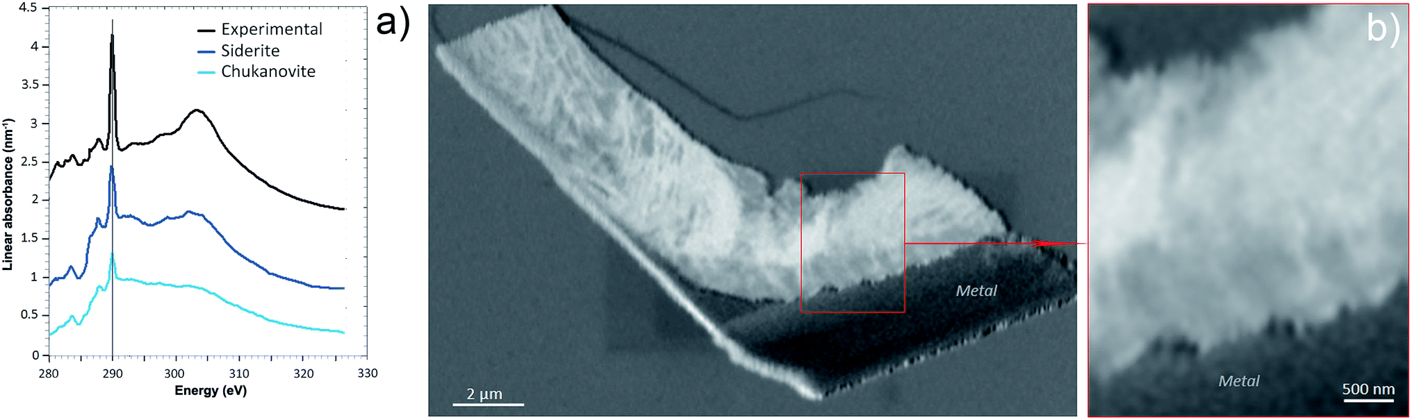Fig. 3 STXM characterization on the interfacial film between iron and corrosion products for the Arcorr2008 sample. (a) Spectrum extracted from the carbonate zone compared to siderite and chukanovite as references at the C K edge. (b) Image difference map (290–280 eV) of the thin film obtained from the carbonate spectra acquired at the C K edge.

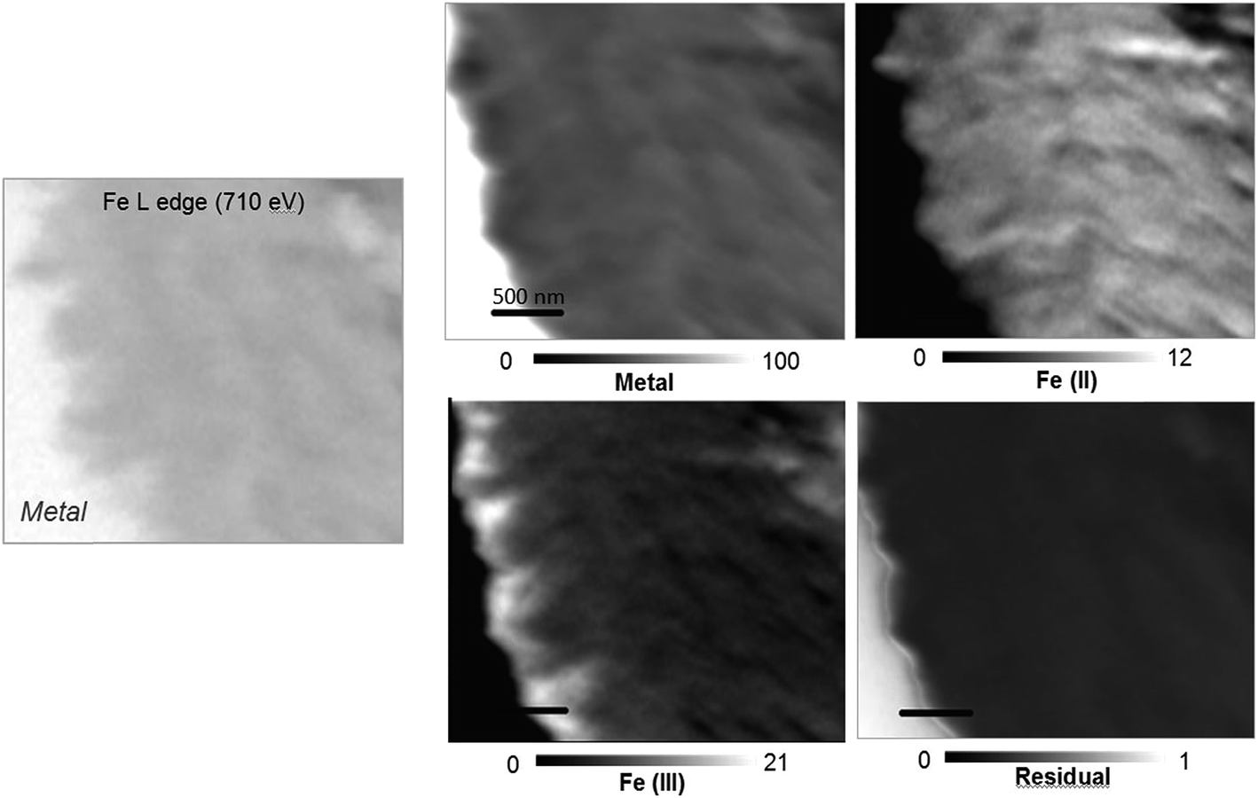Fig. 4 STXM characterization on the interfacial film between iron and corrosion products for the Arcorr2008 sample: Fe L-edge map (710 eV) and SDV component maps of the species Fe^(III), Fe^(II) and Fe⁽⁰⁾ obtained in comparison with the siderite, maghemite and metal reference spectra obtained in a zone of the thin film. The grey scales indicate the equivalent thickness (nm) on the Fe^(II), Fe^(III) and Fe⁽⁰⁾ component maps and the optical density on the residual map.

Fig. 5 STXM characterization of the thin film for the Arcorr2008 sample: color-coded Fe⁽⁰⁾, Fe^(II) and Fe^(III) component maps (SDV) of various regions superimposed on an image difference map (290–280 eV) of the thin film, based on the carbonate spectra acquired at the C K-edge.

Fig. 6 STXM characterization of the thin film for the Arcorr2008 sample: curve fits of the average spectra obtained on the outer (a) and interfacial (b) layers.

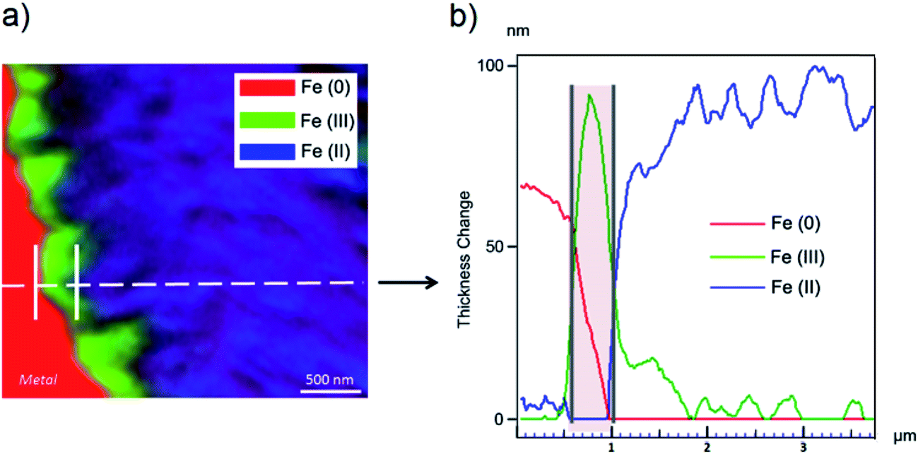Fig. 7 STXM studies of the thin film for the Arcorr2008 sample: (a) color-coded Fe⁽⁰⁾, Fe^(II) and Fe^(III) composite map and (b) profile of the line giving the thicknesses of each component, point by point (every 10 nm) around the metal interface.

3.2. The Batx setup

Analysis of the corrosion interface for the Batx sample was complicated by cracks causing the outer layer of corrosion products to fall away as soon as the iron rod was removed from the autoclave. In the areas where these outer parts were still attached, a layer of corrosion products with a thickness of about 350 μm was observed (Fig. 8a). The most internal part of the “Dense Product Layer” (that nearest to the metal), had an average thickness of about 100 μm (Fig. 8b) and seems rather massive. The outer part of the corrosion products layer showed a highly porous pattern.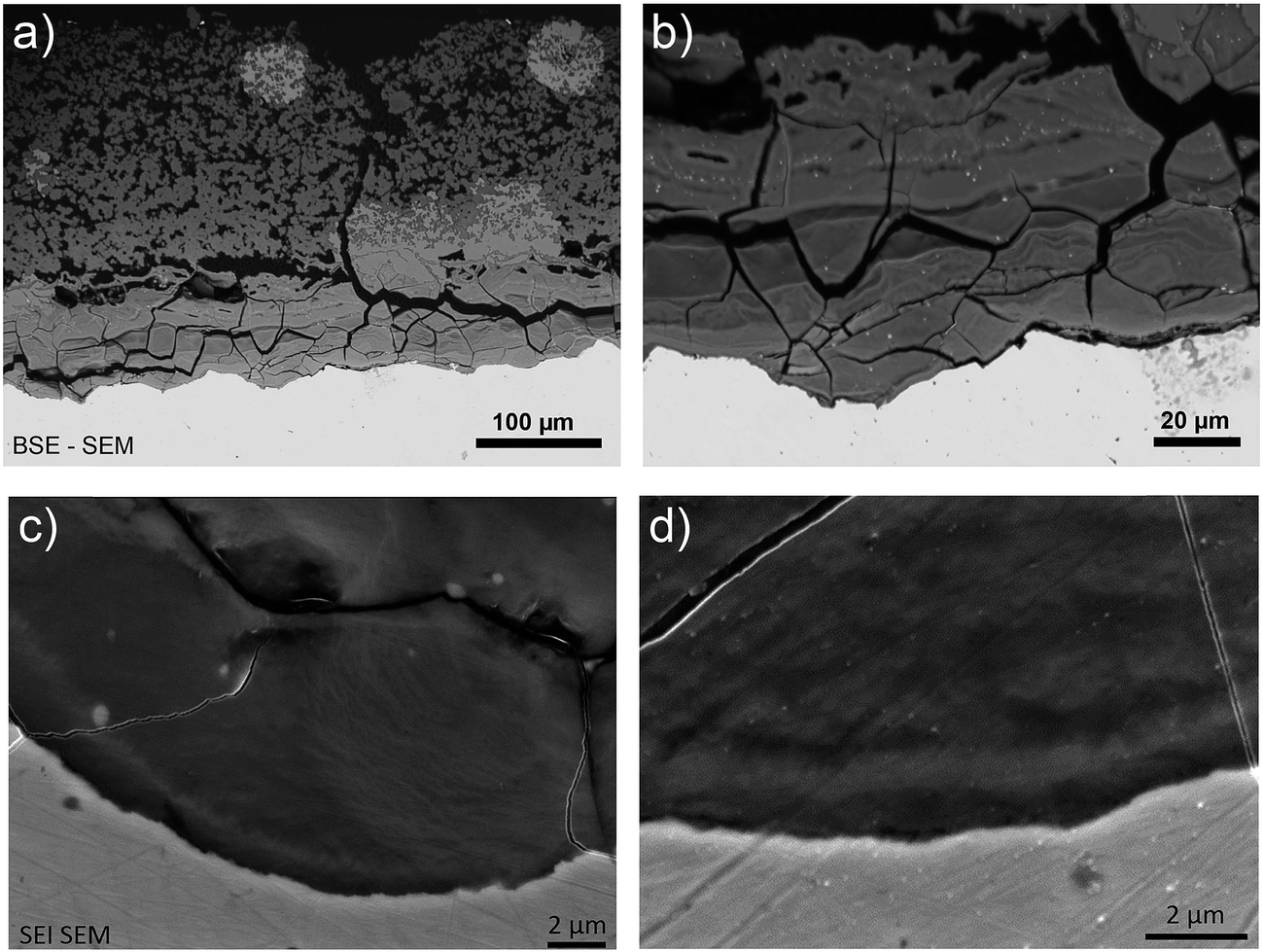

Fig. 8 SEM-FEG BSE micrographs of the metal/corrosion product interface on a cross-section of the Batx sample.

According to the EDS maps (Fig. 9a), outer part of the corrosion products layer contained Fe and Si in spatially varying amounts (from 6 to 21 at%) in addition to O. These cations were distributed in layers several tens of μm thick. In addition to these main elements, small nodules of S-containing corrosion products (where S amounted to up to 10 at%), and occasionally, Mn-rich spots (amounting to up to 7 at%) were identified. These inclusions may have corresponded to former precipitates from the metallic substrate, but the possibility that S may have been of exogenous origin cannot be ruled out.

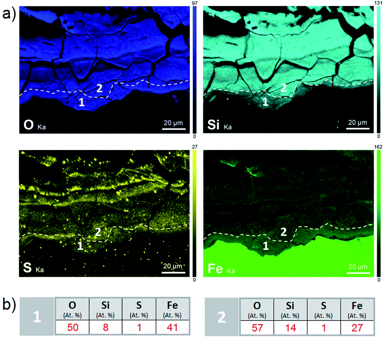Fig. 9 (a) EDS maps of the metal/corrosion product interface on a cross-section of the Batx sample, where O (Kα) is presented in blue, Si (Kα) in light blue, S (Kα) in yellow and Fe (Kα) in green, and (b) average quantification of EDS point analyses performed at two points on the metal/corrosion product interface.

The μRaman spectra obtained in the external porous part of the corrosion products layer clearly showed the presence of siderite (FeCO₃ – giving a peak at 1080 cm⁻¹). The EDX data indicate that this phase was sometimes doped with Mg (1 at%) and Ca (2.5 at%). In the internal part of the corrosion product layer, μRaman spectroscopy showed the presence of chukanovite with a typical band at 1070 cm⁻¹ (Fig. 10c) in most of the internal part of the layer of corrosion products (in blue in Fig. 10b). No spectrum could be obtained for the solids containing Si and S, presumably because these phases had an extremely weak Raman scattering. The μRaman spectra obtained at the metal/corrosion product interface showed the coexistence of magnetite (at 500 and 670 cm⁻¹) and maghemite (at 720 cm⁻¹) (Fig. 10b and d). This interfacial layer of Fe^(III) oxides was observed along the whole interface. It had a thickness of up to 1 μm in some places (Fig. 10b) but seemed to be much thinner in other places. This interfacial layer was not found to coincide with the internal Si-depleted zone.

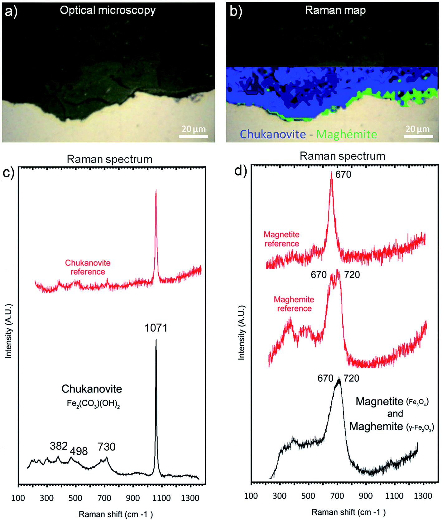Fig. 10 (a) Optical microscopy photograph and (b) μRaman map of chukanovite (in blue) and magnetite (in green) of the metal/corrosion product interface in a cross-section of the Batx sample. Also shown are representative μRaman spectra of some corrosion products: (c) chukanovite Raman spectra of the internal layer of corrosion products and (d) mixed magnetite-maghemite Raman spectra of the interfacial layer.

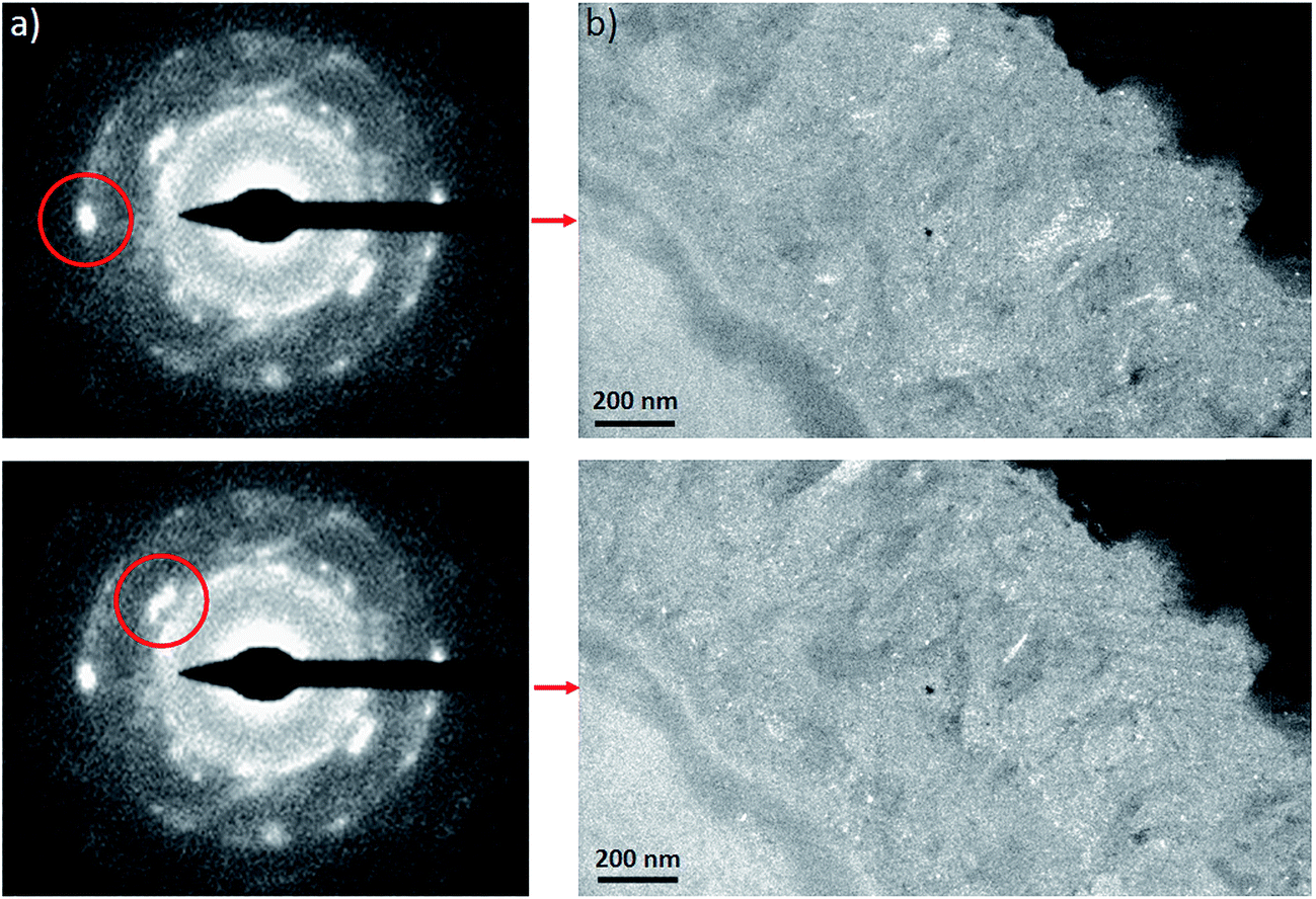
A thin cross-section of the metal/corrosion product interface was obtained by FIB (Fig. 11a). TEM micrographs and EDS-STEM elemental mapping showed the presence of two layers with different contrasts, separated by two C-rich fringes which corresponded to resin-filled pores in the thin film and were no longer taken into consideration (Fig. 11a). There was a difference in the C content between the EDX spectra obtained from the two layers separated by the fringes (zones 1 and 2 in Fig. 11c and d). This confirms that the outer part of the thin film had a higher C content. The O/Fe ratio was indeed lower in the inner layer (measuring about 1 μm in thickness), than in the outer layer. In addition, the inner layer (which probably corresponded to the oxide interfacial layer identified by μRaman spectroscopy) was found to be Si-free. Si was detected only in the outer layer (Fig. 11b), which was probably the outer zone identified by μRaman spectroscopy.

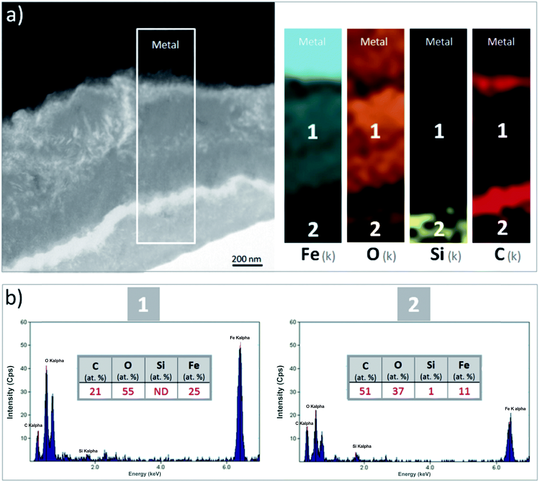Fig. 11 (a) TEM micrograph and EDS-STEM elemental mapping of Fe, O, Si and C and (b) average quantification of EDS punctual analyses performed in two areas of the metal-corrosion product interface in the Batx sample.

The electron diffraction patterns obtained on part of the inner layer 200 nm in diameter (Fig. 12a and b) were consistent with the presence of both magnetite and maghemite. These two phases can only be discriminated by the peak at 1.40 Å, which was visible only in the diffraction pattern of maghemite (Fig. 12d). The electron diffraction patterns obtained on the outer layer of the thin film are consistent with the presence of chukanovite.

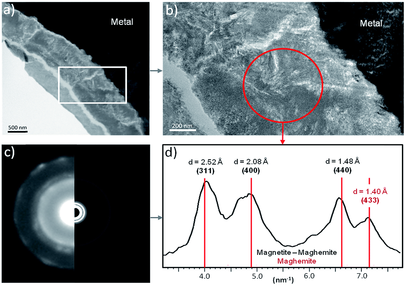Fig. 12 TEM analysis of the thin film originating from the Batx sample: (a) bright-field images of the metal/corrosion product interface and (b) of the interfacial layer with the diffraction area, (c) diffraction pattern obtained on the interfacial layer with (d) the corresponding radially integrated diffraction data.

The dark field images (Fig. 13b) obtained by selecting a particular diffraction spot (Fig. 13a) only show up a subset of crystals having a Bragg reflection at a given orientation, which enabled us to differentiate more clearly between selected crystalline orientations. Based on these micrographs, the interfacial layer was found to consist mainly of randomly oriented crystals a few nm in size.

Fig. 13 TEM analysis of the thin film originating from the Batx sample: (a) electron diffraction patterns of magnetite in the interfacial layer and (b) dark-field images obtained using particular reflections of magnetite obtained by moving the objective aperture around and selecting the most clearly visible diffraction spot (surrounded).

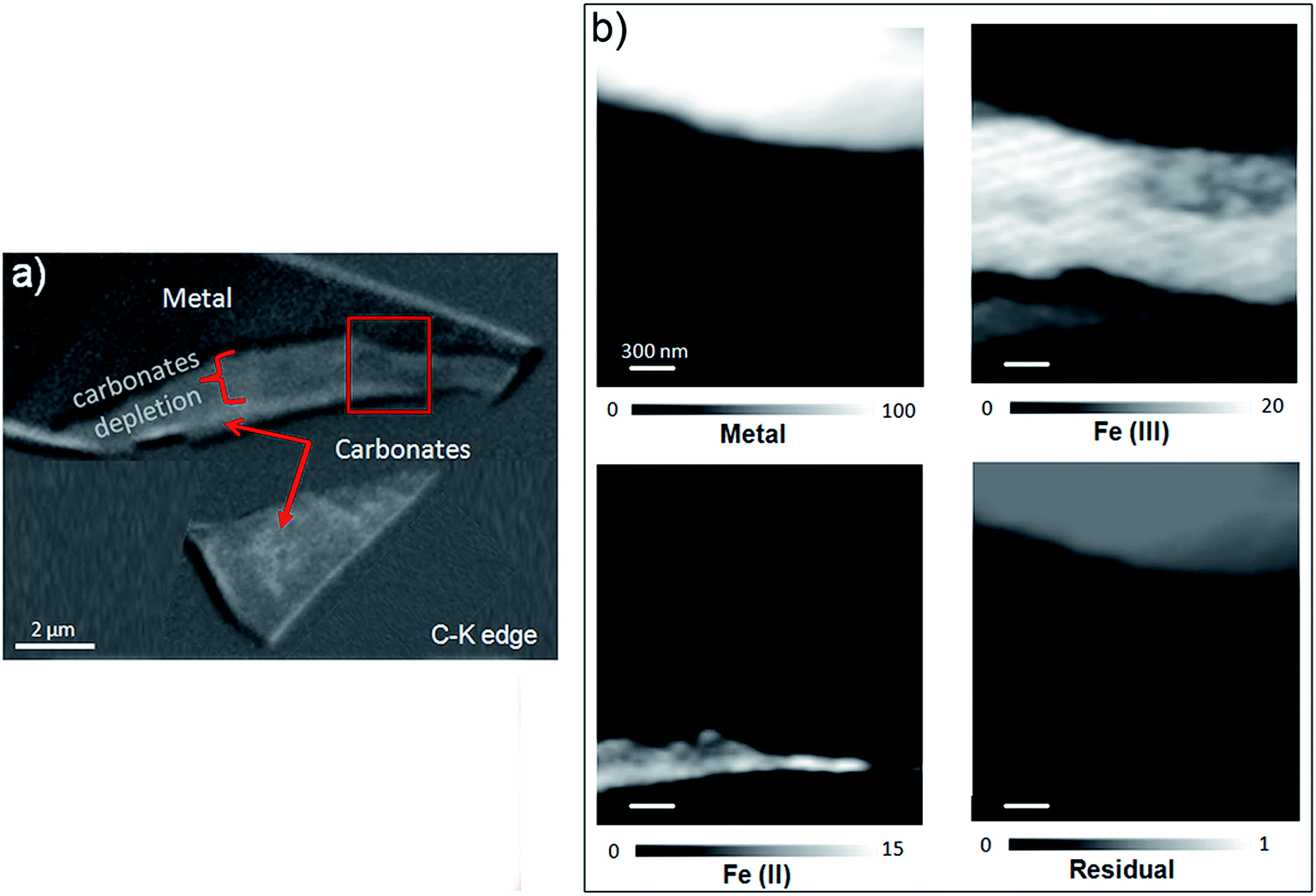
This thin film was also studied by STXM. As the image difference map of the C K edge (290–280 eV) shows (Fig. 14a), the interfacial layer lacked C, and differed from the outer area, which gave a slightly brighter image and was found to contain carbonate. In the component maps of Fe^(III), Fe^(II) and Fe⁽⁰⁾ species (Fig. 14c), the interfacial layer could be seen to have consisted mostly of Fe^(III) species, while the outer layer consisted mainly of Fe^(II) species.

Fig. 14 STXM characterization of the Batx interfacial thin film. (a) Image difference map (290–280 eV) of the thin film obtained from the carbonate spectra collected at the C K-edge. (b) SDV component maps of the Fe(III), Fe(II) and Fe(0) species obtained with the siderite, maghemite and metal reference spectra in part of the thin film (the grey scales indicate the equivalent thickness (nm) on the Fe(0), Fe(II), and Fe(III) component maps and the optical density on the residual map).

The best curve fit (χ² = 0.3) of the spectrum obtained on the interfacial zone contained contributions from both magnetite (14 nm) and maghemite (7.5 nm) (Fig. 15b). According to the best curve fit (χ² = 0.04), the spectrum corresponding to the outer layer corresponded to a combination of chukanovite (9 nm) and siderite (8 nm), indicating that Fe^(II) carbonates were the predominant species (Fig. 17c). However, there was also significant Fe^(III) oxides contribution (6 nm), possibly due to contamination from the nearby interfacial layer. The milling of the film made it possible to keep only a thin part of the outer layer, which was partly mixed with the Fe^(III) oxide layer. Another explanation for the presence of Fe^(III) oxides might be that the presence in the outer layer of Fe^(II,III) ferrosilicates that were not detected by μRaman spectroscopy (Fig. 16).

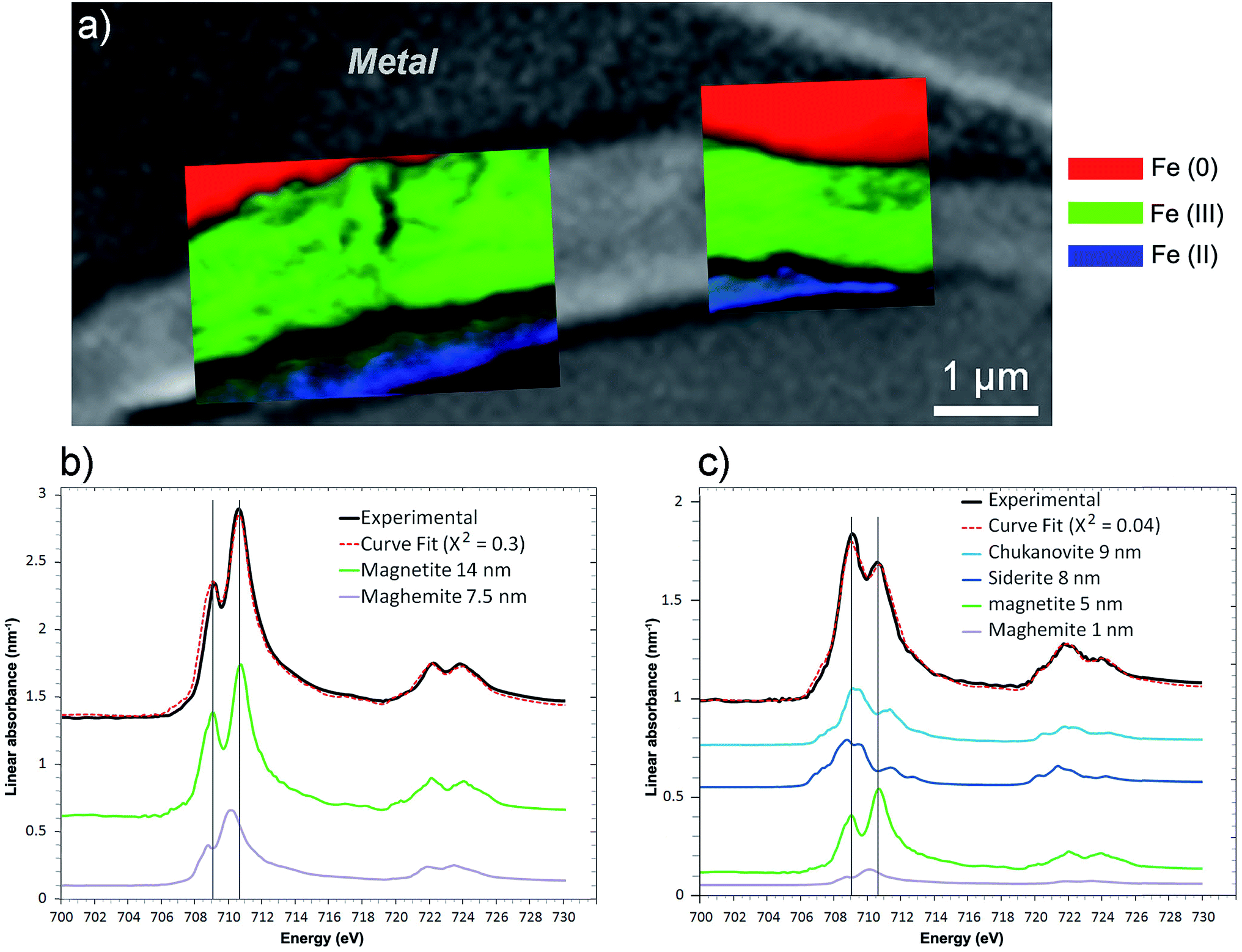Fig. 15 STXM characterization of the thin film for the Batx sample. (a) Composite color-coded maps of the Fe⁽⁰⁾, Fe^(II) and Fe^(III) components based on SDV maps of various regions of the thin film superimposed on the image presented in Fig. 14a. Curve fits of the average spectrum obtained on the (b) interfacial and (c) outer layers, along with the reference spectra used (metal, chukanovite, siderite, magnetite and maghemite) and the equivalent thicknesses deduced (in nm).

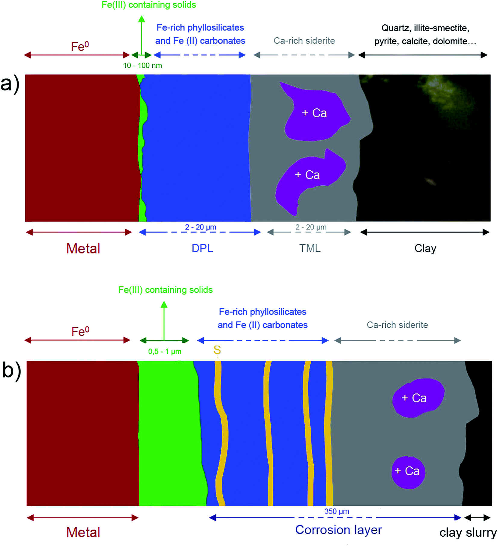Fig. 16 Diagram of the corrosion patterns at work in the two systems (a) Arcorr2008 and (b) Batx.

3.3. Comparison and interpretation of results

In both samples, the outer layers of corrosion products were made of carbonates, hydroxycarbonates and poorly ordered Fe-silicates. Chukanovite (Fe₂CO₃(OH)₂) was the main compound detected in the most internal part of the outer layers, while the outer part was found to mainly consist of Fe^(II) carbonates, siderite (FeCO₃), ankerite ((Fe, Ca, Mg)CO₃) and Fe-silicates. The Fe-silicate phases were more difficult to identify probably because of their low crystallinity.

Despite the same corrosion time, the thicknesses of these layers in the two systems were found to differ by up to 40 μm for the Arcorr2008 sample and 350 μm for the Batx sample. This difference could be explained by the difference of compactness of the medium in contact with the metal (see below). Thick layers of corrosion products, mainly of carbonates, are known to form in carbonated media^33,34 and at compact clay interfaces.^9,35,36 Several studies have shown that the growth and densification (decreasing levels of porosity) of this layer generate a transport barrier in the species involved in the corrosion process, which cover part of the available metallic surfaces.³⁷ The hindering effects of this barrier contribute to the decrease in the corrosion rate. The first stage in the corrosion process, corresponding to the growth of a carbonate film on the metal substrate, has been investigated in several short-term studies, mostly dealing with CO₂ corrosion. Nešić et al. (2003) observed a decrease in the corrosion rate down to 30 μm per year in a mild steel after 0.5 days in a pH 6.6 solution saturated with CO₂ (0.54 bar) at 80 °C in the presence of dissolved Fe²⁺ species (250 ppm). The low corrosion rate was attributed to the formation of a dense layer of siderite on the mild steel. Zhao et al. (2009) observed a decrease in the corrosion rate from 15 mm per year to 1530 μm per year for a P110 steel immersed in carbonated water ([HCO₃⁻] = 0.15 g L⁻¹, [Fe²⁺] = 0.1 g L⁻¹, [Fe³⁺] = 0.3 g L⁻¹) for 10 days, which was also attributed to the formation of a dense carbonate film.³³ The duration of these studies was very short in comparison with the studies presented here. This stage probably corresponds to the incubation stage observed by corrosion rate monitoring on Arcorr2008 (see 2.1. and literature⁹)

Electrochemical measurements performed on corroded steel in clay media for 8 months³⁸ and on Fe electrodes immersed in a carbonate/bicarbonate solution¹¹ suggested that a further decrease in the corrosion rate may be due to the presence of very dense films at the boundary between the metal and the thick outer layers. The same decrease was observed by corrosion monitoring performed on Arcorr2008,⁹ showing a progressive drop of the corrosion rate to 0.3 μm per year after 700 days. The presence of this dense film is corroborated by our detection of interfacial layers consisting mainly of oxides with a spinel structure (magnetite and maghemite) in both of our samples. An interfacial layer of a similar kind to that observed here was also formed on archaeological artefacts corroded for 500 years under anoxic carbonated conditions,^20,28 which suggests that the formation of this interfacial layer is actually quite a common occurrence under anoxic carbonated conditions. However, the nature, thickness and density of the interfacial layers seem to differ between the two systems studied here. In the Batx sample, the interfacial layer is a mixture of well-crystallized magnetite and maghemite, as clearly shown by μRaman spectroscopy, electron diffraction, and STXM analyses. The thickness of this layer ranges between 500 nm and 1 μm. In the Arcorr2008 sample, the interfacial layer was much more difficult to characterize because it was very thin. The STXM measurements suggested that the layer was thinner than 100 nm, while the TEM investigations suggested that it had a thickness of about 10 nm and possibly showed poor crystallinity. In addition, STXM data showed the presence of Fe^(III) species in the outer carbonated corrosion products, even at a distance of several 100 nm from the interfacial layer. This may have been due to the local occurrence of phases containing Si, some of which could contain both Fe^(II) and Fe^(III).³² These differences of composition between the interfacial fringes of the two systems could be explained by differences in the local conditions at the metal interface. Actually, as stated by Han et al.¹⁴ the formation of interfacial layers depends on several factors such as the composition of the alloy, the local pH, the presence of cations and anions, the fluid dynamics, etc. Difference in the porosity of the outer layers and of compactness (permeability) of the contacting media of the two systems might also account for variations in the nature of the interfacial layer.

Some authors have put forward possible explanations for the formation of interfacial layers based on an increase in pH at the metal interface due to water hydrolysis and hindered transport of H⁺ through the outer corrosion products.^14,15,39,40 Because of that, the local pH level under an iron carbonate layer can be quite high (7 > pH > 9) even if the bulk pH is acidic (e.g. pH 4–6).¹⁴ These pH values change the nature of Fe-containing predominant solids from carbonates (or silicates) to iron oxides causing the formation of a passivating interfacial layer. SEM data and optical observations confirm that the outer corrosion layer which formed on the Batx sample corroded in a clay slurry was considerably more porous than that observed on the Arcorr2008 sample (see Fig. 1 and 8) corroded in compacted clay. The highly compacted structure of the Arcorr2008 setup resulting in a less porous outer layer may have hindered the fast transport of the species and changing thermodynamic conditions at the interface more quickly, thus stabilising the oxide interfacial layer. The protective role of the interfacial layer has been described in archaeological samples on which re-corrosion experiments were performed in D₂O for three months. The results obtained in these experiments showed that water did not permeate this layer, which confirmed the hypothesis that a kinetic control might be exerted by solid-state transport processes in the interfacial layer.²⁰ The growth of the interfacial layer, which gradually restrains solid-state transport, can cause a significant decrease in the corrosion rate.^21,41–43 It is worth noting that in the case of the Batx sample, the passive film cannot correspond to the entire thickness of the oxide layer identified here, which is several orders of magnitude thicker than a passive film. It seems very probable that only a small dense part of this interfacial layer may play this passivation role.

Previous authors have underlined the influence of compactness of the environment on the behaviour of corrosion systems and modelled mechanisms possibly at work in physically constrained systems in other environments (such as concrete, or here, compacted clay).⁴⁴ In this model after a certain time, the progressive clogging of the pores of the outer corrosion products hinder chemical transport, which eventually controls the kinetics and significantly decreases the corrosion rate. This could be the case for Arcor2008. In the case of the Batx experiment that took place in a non-confined environment, the porosity of the outer corrosion products should remain fairly high, thus the kinetics are only controlled by the interfacial layer, resulting in higher corrosion rates than in a non-compacted environment. The fact that the interfacial oxide layer was thicker in BatX case may be attributable to this higher corrosion rate, as suggested in previous modelling studies.²¹

4. Conclusions

Two experimental systems involving metal iron corroded for several years in an anoxic carbonated medium, which mimicked the conditions pertaining to the deep storage of nuclear wastes were studied. Several conclusions can be drawn from the results of the present study:

- The presence of an interfacial layer consisting of a mixture of Fe^II/Fe^III spinel oxide was detected by combining micro- and nanoscale methods of characterisation. This finding confirms previous electrochemical results obtained in laboratory experiments^13,21,38 and recent studies on archaeological nails.²⁰

- This low-porosity interfacial layer may partly control the corrosion process via a solid-state transport process, as suggested by several authors, including those who performed re-corrosion experiments on archaeological artefacts.

- However, the structural properties of the passivation layer alone may not suffice to explain the differences in behaviour observed between compact interfaces (quasi-passivation) and slurries (significant residual corrosion rates).

- The differences between the corrosive environments (compacted clay vs. clay slurry) studied here were of great importance. In fact, the transport-hindering properties of compacted clay systems, leading to a progressive clogging of the outer carbonate layer must have promoted the establishment of conditions favouring the formation of a passive Fe-oxide layer as well as a steady decrease in the corrosion rate with time.

Acknowledgements

We thank C. Bataillon, for setting up the experimental tests and providing the samples. B. Grenut, C. Lascoutouna, P. Vigier ang J-P Gallien are acknowledged for their assistance with the sample preparation, D. Troadec at IEMN for helping with the thin film preparation. We are most grateful to D. Crusset, N. Michau, Ch. Martin and F. Foct for their comments and suggestions. The authors acknowledge the help of E. Leroy and J. Bourgon at ICMPE with the TEM measurements, E.Vega and C. Blanc for their assistance with the SEM-FEG analyses, Jtime. This work was partly funded by the Groupement de Laboratoires “Verre-Fer-Argile” at French National Agency for the Management of Radioactivity and supported by the CEA, and Electricité de France (EDF).

References

1. F. F. Eliyan and A. Alfantazi, Corrosion, 2014, 70, 880–898.
2. D. A. Scott and G. Eggert, Iron and Steel in Art: Corrosion, Colorants, Conservation, Archetype Publications Ltd, Plymouth, 2009.
3. P. Dillmann, D. Watkinson, E. Angelini and A. Adriens, Corrosion and conservation of cultural heritage metallic artefacts, Woodhead publishing, Oxford, 2013.
4. E. Shelton, A. B. Rothwell and R. I. Coote, Met. Technol., 1983, 10, 234–241.
5. F. Farelas, M. Galicia, B. Brown, S. Nesic and H. Castaneda, Corros. Sci., 2010, 52, 509–517.
6. A. Clanfield, F. Cattant, D. Crusset and D. Feron, Mater. Today, 2008, 11, 32–37.
7. D. Feron, D. Crusset and J. M. Gras, Corrosion, 2009, 65, 213–223.
8. D. Feron, D. Crusset, J.-M. Gras and D. D. Macdonald, Prediction of long term corrosion behaviour in nuclear waste systems, ANDRA, Chatenay-Malabry, 2004.
9. M. Schlegel, C. Bataillon, F. Brucker, C. Blanc, D. Prêt, E. Foy and M. Chorro, Appl. Geochem., 2014, 51, 1–14.
10. M. Saheb, D. Neff, J. Demory, E. Foy and P. Dillmann, Corros. Eng., Sci. Technol., 2010, 45, 381–387.
11. E. B. Castro, J. R. Vilche and A. J. Arvia, Corros. Sci., 1991, 32, 37–50.
12. C. M. Rangel, I. T. Fonseca and R. A. Leitão, Electrochim. Acta, 1986, 31, 1659–1662.
13. C. Bataillon, C. Musy and M. Roy, J. Phys. IV, 2001, 267–274.
14. J. Han, S. Nešić, Y. Yang and B. N. Brown, Electrochim. Acta, 2011, 56, 5396–5404.
15. J. Han, D. Young, H. Colijn, A. Tripathi and S. Nešicć, Ind. Eng. Chem. Res., 2009, 48, 6296–6302.
16. J. K. Heuer and J. F. Stubbins, Corros. Sci., 1999, 41, 1231–1243.
17. A. J. Davenport, L. J. Oblonsky, M. P. Ryan and M. F. Toney, J. Electrochem. Soc., 2000, 147, 2162–2173.
18. L. J. Oblonsky, M. P. Ryan and H. S. Isaacs, Corros. Sci., 2000, 42, 229–241.
19. A. Michelin, E. Drouet, E. Foy, J. J. Dynes, D. Neff and P. Dillmann, J. Anal. At. Spectrom., 2013, 28, 59–66.
20. Y. Leon, M. Saheb, E. Drouet, D. Neff, E. Foy, E. Leroy, J. J. Dynes and P. Dillmann, Corros. Sci., 2014, 88, 23–35.
21. C. Bataillon, F. Bouchon, C. Chainais-Hillairet, C. Desgranges, E. Hoarau, F. Martin, S. Perrin, M. Tupin and J. Talandier, Electrochim. Acta, 2010, 55, 4451–4467.
22. E. C. Gaucher, C. Tournassat, F. J. Pearson, P. Blanc, C. Crouzet, C. Lerouge and S. Altmann, Geochim. Cosmochim. Acta, 2009, 73, 6470–6487.
23. C. Bataillon, Procédure de réalisation d'une solution synthétique de Bure a 90 °C, Report NT DPC/SCCME 08–412.A, Saclay, 2008.
24. D. Neff, L. Bellot-Gurlet, P. Dillmann, S. Reguer and L. Legrand, J. Raman Spectrosc., 2006, 37, 1228–1237.
25. D. R. G. Mitchell, Microsc. Res. Tech., 2008, 71, 588–593.
26. K. V. Kaznatcheev, C. Karunakaran, U. D. Lanke, S. G. Urquhart, M. Obst and A. P. Hitchcock, Nucl. Instrum. Methods Phys. Res., Sect. A, 2007, 582, 96–99.
27. J. A. Brandes, S. Wirick and C. Jacobsen, J. Synchrotron Radiat., 2010, 17, 676–682.
28. A. Michelin, E. Drouet, E. Foy, J. J. Dynes, D. Neff and P. Dillmann, J. Anal. At. Spectrom., 2013, 28, 59–66.
29. J. J. Dynes, T. Tyliszczak, T. Araki, J. R. Lawrence, G. D. W. Swerhone, G. G. Leppard and A. P. Hitchcock, Environ. Sci. Technol., 2006, 40, 1556–1565.
30. J. Störh, NEXAFS spectroscopy, Springer, New-York, 1992.
31. A. P. Hitchcock, http://unicorn.mcmaster.ca.
32. P. Dillmann, S. Gin, D. Neff, L. Gentaz and D. Rebiscoul, Geochim. Cosmochim. Acta, 2016, 172, 287–305.
33. G.-X. Zhao, X.-H. Lu, J.-M. Xiang and Y. Han, J. Iron Steel Res. Int., 2009, 16, 89–94.
34. S. Nesić, J. Postlethwaite and M. Vrhovac, Corros. Rev., 1997, 15, 211.
35. M. L. Schlegel, C. Bataillon, K. Benhamida, C. Blanc, D. Menut and J.-L. Lacour, Appl. Geochem., 2008, 23, 2619–2633.
36. M. Schlegel and C. Blanc, Characterization Of The Iron-Clay Corrosion Interface From Corridda Setups, Report NT DPC/SCP 10–371 indice A, CEA/DEN/DANS/DPC/SCP/LRSI, 2010.
37. S. Nešić, Corros. Sci., 2007, 49, 4308–4338.
38. F. A. Martin, C. Bataillon and M. L. Schlegel, Proceedings of the Third International Workshop on Long-Term Prediction of Corrosion Damage in Nuclear Waste Systems, 2008, vol. 379, pp. 80–90.
39. J. Han, B. Brown, D. Young and S. Nešić, J. Appl. Electrochem., 2010, 40, 683–690.
40. Y. Leon, M. Saheb, E. Drouet, D. Neff, E. Foy, E. Leroy, J. J. Dynes and P. Dillmann, Corros. Sci., 2014, 88, 23–35.
41. C. Y. Chao, L. F. Lin and D. D. Macdonald, J. Electrochem. Soc., 1981, 128, 1187–1194.
42. M. Bojinov, G. Fabricius, T. Laitinen, K. Mäkelä, T. Saario and G. Sundholm, Electrochim. Acta, 2000, 45, 2029–2048.
43. A. Seyeux, V. Maurice and P. Marcus, J. Electrochem. Soc., 2013, 160, C189–C196.
44. D. D. Macdonald, B. Kursten and G. R. Engelhardt, ECS Trans., 2013, 50, 457–468.

---