 Open Access Article
Investigation into the pharmacokinetic–pharmacodynamic model of Zingiberis Rhizoma/Zingiberis Rhizoma Carbonisata and contribution to their therapeutic material basis using artificial neural networks
Sujuan Zhou ab,
Jiang Meng*c and
Bo Liu*a
aDepartment of Automation, Guangdong University of Technology, Guangzhou, 510006, China. E-mail: csbliu@189.cn; Tel: +86 020 39322469
bCollege of Medical Information Engineering, Guangdong Pharmaceutical University, Guangzhou, 510006, China. E-mail: susona2002@163.com; Tel: +86 020 39352207
cCollege of Traditional Chinese Medicine, Guangdong Pharmaceutical University, Guangzhou, 510006, China. E-mail: jiangmeng666@126.com; Tel: +86 020 39352169
First published on 12th May 2017
Abstract
Zingiberis Rhizoma (ZR) and Zingiberis Rhizoma Carbonisata (ZRC) are two varieties of processed ginger, which are widely used in traditional Chinese medicine (TCM) and exhibit varying drug efficacy. In this study, an Artificial Neural Network (ANN) model was developed for simultaneously characterizing the pharmacokinetics (PK) and pharmacodynamics (PD) of ZR/ZRC. In order to evaluate the relative contribution of the ZR/ZRC drug concentration of its main components to its drug efficacy, connection weights method and Mean Impact Value (MIV) have been introduced. The results have shown that sequences of the contribution value calculated by these two methods was same overall and indicated that the active components of ZR and ZRC exhibited opposite drug efficacy after processing. In conclusion, ANN was found to be a powerful tool that linked PK and PD profiles of ZR/ZRC with multiple components; it also provided a simple method to identify and rank the relative contribution of each to the multiple therapeutic effects of the drug.
Introduction
Zingiberis Rhizoma (ZR, Ganjiang) is a well-known herbal medicine and edible plant extensively used in China, India and other South-Eastern Asian countries since thousands of years.1,2 It is the dried rhizome of Zingiber officinale Rosc. Zingiberis Rhizoma Carbonisata (ZRC) is produced by stir-frying ZR in a utensil and heating to a temperature that is high enough to turn the bark's surface black-brown.3,4 According to the TCM theory, ZR has the effect of warming and dispelling cold, venation restoration and warming the lungs to reduce watery phlegm. It can be used to cure cold, vomiting, diarrhea, coughs, etc. While ZRC has the function of warming meridian and hemostasis, so it is used for hemorrhage of deficiency cold, hematochezia, metrorrhagia, and metrostaxis.3,5,6The study of pharmacokinetic (PK)–pharmacodynamic (PD) characteristics of ZR and ZRC is to investigate the mechanism of their pharmacodynamics and therapeutics.7 For traditional Chinese medicines containing multiple components and therapeutic targets,8,9 the process of developing PK–PD models represents a formidable task and may face methodologic difficulties.10 Conventional researches on PK–PD mostly rely on known models. That is, PK–PD data should be processed based on the established models and then results could be used in turn to correct the models. This would consume time and money.11 In contrast, ANN models have lower inaccuracy, cost, and time-consumption.12,13
In recent years, Artificial Neural Network (ANN) has been used extensively in the PK–PD analysis model of Chinese herbals for its non-linear fitting ability.14,15 Without any supposed model, ANN can help to approach a mathematical model16 reflecting the inherence regularity of experimental data after several times of iterative computation based on the relationship between input and output data. There are different structure types of ANN, in which Back-Propagation (BP)17 and Radical Basis Function (RBF)18,19 are the two most widely used methods.20 Moreover, General Regression Neural Network (GRNN)21,22 is an improved method of RBF. Herein, we utilized a PK/PD model of ZR/ZRC based on BP and GRNN by selecting time as the correlation factor of drug concentration and efficacy. Furthermore, the relationships between drug concentration of main components and drug efficacy indexes such as TXB2/6-keto-PGF1α and Thromboxane B2 (TXB2) can be analyzed with the aid of this model.
But determining the contribution of each independent variable in ANN models still remains unanswered. Neural network technique is cited in the literature as a ‘Black Box’23 approach and is often criticized for lack of interpretability of the network weights obtained during the model building process. This arises from the fact that internal characteristics of a trained network is a set of numbers, which becomes very difficult to relate to the application in a meaningful fashion.24 Considering this problem, methods to determine the relative importance of variables in a neural network model have been proposed and applied by numerous authors in several research fields:25,26 perturb, profile, connection weights and partial derivatives.
One of the most important objectives of this study was to evaluate the relative contribution of ZR/ZRC drug concentration of main components to their drug efficacy. Only considerable reports on neural networks technique are available to explore in this field. In the present study, connection weights method and Mean Impact Value (MIV) have been introduced to assess the importance of axon connection weights and contribution of input variables in ANN. Ultimately, the efficacious material basis and process mechanism of ZR/ZRC can be illuminated.
Data source
All experiments reported in the following section have been performed in compliance with animal protection law of China and institutional guidelines of National Natural Science Foundation of China (NSFC). The institutional committees from Faculty and NSFC panels have approved the experiments reported in the present study. All these data were obtained from the research conducted by the Research Group of Jiang Meng supported by the Project of National Natural Science Foundation of China (No. 81102809).Male Sprague-Dawley (SD) rats (weighing 300 ± 20 g), purchased from Experimental Animal Center of Guangdong Province, have been divided into four groups, namely black group, model group (deficiency-cold and bleeding rats group), ZR treated animals and ZRC treated animals. Blood was collected at different time after the seventh day administration from rats, such as 0.083 0.25, 0.5, 0.75, 1, 2, 3, 4, 5, 6, 7, 10 and 12 h.
Seven compounds of blood (zingiberone, 6-gingerol, 8-gingerol, 6-ginger-ketone, 6-shogaol, diacetoxy-6-gingerdiol and 10-gingerol) were quantified using high-performance liquid chromatography method. Chromatographic conditions: Shimadzu LC-20AT system with DAD (Shimadzu Corp., Japan) was used for all analyses. Chromatographic separations were carried out at 30 °C on an Ultimate TM XB-C18 column (4.6 × 250 mm, 5 μm). The mobile phase consisted of acetonitrile (A) and water containing 0.1% phosphoric acid (B). The gradient elution program was as follows: 0–10 min, 10% A; 10–20 min, 25% A; 20–45 min, 35% A; 45–80 min, 75% A; 80–90 min, 98% A; 90–95 min, 10% A. The flow rate was 0.6 mL min−1 and the injection volume was 20 μL.
At the same time, pharmacodynamics was also evaluated with TXB2/6-keto-PGF1α and TXB2. TXB2/6-keto-PGF1α and TXB2 of rats' serum were determined with enzyme-linked immunoassay detection. The details of the experiment will be published in another study.
PK–PD model construction based on ANN
Construction of BP model
| Time (h) | PK (content/μg ml−1) | PD (%) | ||||||
|---|---|---|---|---|---|---|---|---|
| 6-Gingerol | Zingiberone | 6-Shogaol | 10-Gingerol | 6-Ginger-ketone | Diacetoxy-6-ingerdiol | TXB2/6-keto-PGF1α | TXB2 (%) | |
| a TXB2/6-keto-PGF1α% = (Ctreated animals − Cmodel animal)/(Cmodel animal − Cblack animal) × 100%. TXB2% = (Ctreated animals − Cmodel animal)/(Cmodel animal − Cblack animal) × 100%. | ||||||||
| 0.083 | 1.292 | 2.951 | 0.29 | 0.479 | 0.465 | 0.235 | 12.875 | 37.665 |
| 0.25 | 1.484 | 2.536 | 1.782 | 0.309 | 1.909 | 0.489 | 49.235 | 70.816 |
| 0.5 | 1.618 | 2.472 | 2.479 | 0.203 | 1.966 | 1.27 | 28.287 | 55.68 |
| 0.75 | 3.116 | 6.064 | 3.057 | 0.556 | 5.553 | 0.143 | 17.379 | 43.069 |
| 1 | 2.230 | 7.508 | 3.52 | 1.02 | 3.042 | 1.387 | 37.876 | 63.605 |
| 2 | 2.000 | 6.385 | 5.735 | 0.224 | 8.691 | 3.212 | 64.574 | 82.703 |
| 3 | 2.135 | 3.911 | 4.664 | 1.01 | 11.106 | 2.781 | 88.714 | 93.876 |
| 4 | 1.561 | 2.839 | 2.67 | 1.017 | 8.541 | 1.998 | 56.673 | 77.299 |
| 6 | 1.022 | 2.276 | 3.558 | 0.6 | 6.69 | 1.185 | 63.71 | 82.703 |
| 8 | 0.739 | 1.507 | 3.003 | 0.229 | 3.403 | 0.676 | 40.101 | 65.771 |
| 10 | 0.348 | 1.184 | 1.81 | 0.134 | 1.836 | 0.798 | 38.042 | 63.605 |
| 12 | 0.118 | 0.322 | 0.504 | 0.042 | 0.977 | 0.544 | 22.316 | 48.474 |
| Time (h) | PK content/μg ml−1 | PD (%) | ||||||
|---|---|---|---|---|---|---|---|---|
| 6-Gingerol | 8-Gingerol | 6-Shogaol | 10-Gingerol | 6-Ginger-ketone | Diacetoxy-6-gingerdiol | TXB2/6-keto-PGF1α | TXB2 (%) | |
| a TXB2/6-keto-PGF1α% = (Ctreated animals − Cmodel animal)/(Cmodel animal − Cblack animal) × 100%. TXB2% = (Ctreated animals − Cmodel animal)/(Cmodel animal − Cblack animal) × 100%. | ||||||||
| 0.083 | 5.011 | 0.869 | 0.907 | 0.95 | 0.819 | 1.259 | −15.22 | −10.4687 |
| 0.25 | 6.746 | 1.504 | 1.621 | 0.65 | 1.191 | 1.819 | −13.72 | −8.8083 |
| 0.5 | 11.718 | 2.672 | 2.661 | 0.983 | 1.336 | 0.952 | −1.26 | −0.5777 |
| 0.75 | 10.148 | 0.593 | 3.028 | 1.352 | 2.891 | 1.947 | 6.16 | 2.3823 |
| 1 | 8.086 | 2.994 | 3.515 | 2.169 | 1.787 | 2.791 | −14.84 | −10.2522 |
| 2 | 5.842 | 5.851 | 4.912 | 2.006 | 4.663 | 2.947 | −1.66 | −0.2889 |
| 3 | 8.77 | 4.089 | 2.35 | 1.467 | 6.955 | 1.646 | −6.3 | −3.2489 |
| 4 | 7.597 | 2.507 | 3.121 | 1.012 | 4.463 | 1.107 | −1.42 | −0.6496 |
| 6 | 6.228 | 2.148 | 3.834 | 0.455 | 3.302 | 0.53 | −6.17 | −2.8159 |
| 8 | 4.893 | 0.806 | 2.694 | 0.121 | 2.908 | 0.52 | −14.57 | −9.8191 |
| 10 | 1.869 | 0.169 | 1.772 | 0.064 | 1.719 | 0.307 | −16.17 | −11.8403 |
| 12 | 0.271 | 0 | 0.908 | 0.05 | 0.347 | 0.152 | −16.84 | −12.6345 |
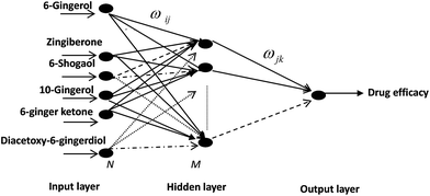
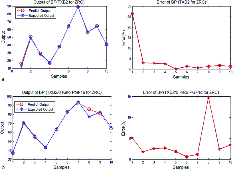
Therefore, selective neural network 6-23-1 topology structure for PK–PD of ZR was determined, where “6” meant six input neurons: 6-gingerol, 8-gingerol, 6-shogaol, 10-gingerol, 6-ginger ketone, diacetoxy-6-gingerdiol, “23” meant hidden-layer neurons number and “1” meant output neurons: values of TXB2/6-keto-PGF1α or TXB2. Similarly, selective neural network 6-16-1 topology structure for PK–PD of ZRC was determined, where “6” meant input neurons: 6-gingerol zingiberone, 6-shogaol, 10-gingerol, 6-ginger, ketone, diacetoxy-6-ingerdiol, “16” meant the hidden-layer neurons number and “1” meant the output neurons: values of TXB2/6-keto-PGF1α or TXB2.
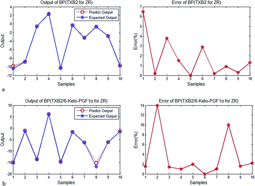 | ||
| Fig. 2 (a) Output and error of BP (TXB2 for ZR). (b) Output and error of BP (TXB2/6-keto-PGF1α for ZR). | ||
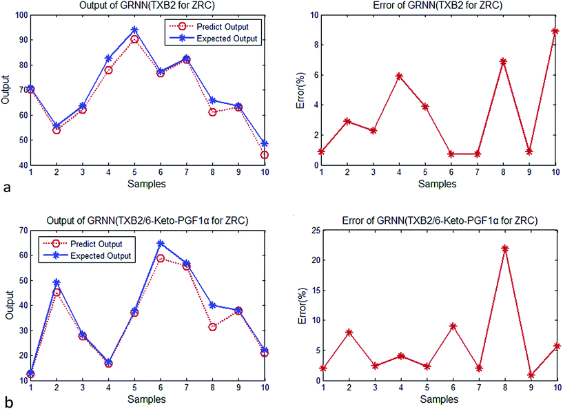
The first step was unsupervised learning to determine the weight value IW1 between input layer and hidden layer; the value of threshold b was determined by the SPREAD constants.
The second step was supervised learning, to generate weight value matrix LW2 between hidden layer and output layer.
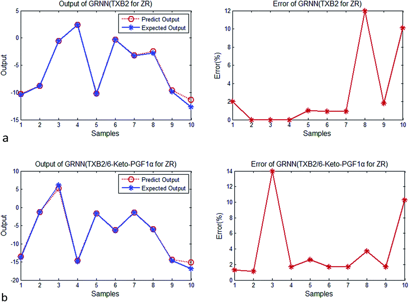 | ||
| Fig. 4 (a) Output and error of GRNN (TXB2 for ZR). (b) Output and error of GRNN (TXB2/6-keto-PGF1α for ZR). | ||
| BP | GRNN | |
|---|---|---|
| Average error | 3.6% | 3.9% |
| Parameter numbers | 5 (or more) | 1 |
| Hidden layer neurons | 23 | Big (equal to nums of train samples) |
Evaluation of relative contributions
Based on above results, PK–PD model constructed using neural networks can effectively predict the relationship between component concentrations and drug efficacy. However, one of the limitations of ANN was its high inability to explicitly know the relations between explanatory variables (input) and dependent variables (output). This was a major reason for them being called as ‘‘black boxes’’.28 In this study, we further explored the relationship between input values and output values, in order to determine the contribution of ZR/ZRC drug concentration of main components to their drug efficacy.For this, connection weights method and Mean Impact Value (MIV) were utilized to solve these problems.
Connection weights method
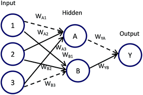
Connection weights method includes four indexes:26 matrix containing input-hidden-output neuron connection weights, connection weights contribution value of input-hidden-output layer, relative contribution of each input neuron to the hidden neuron and relative importance of each input variable.Based on Fig. 6, detailed algorithm of connection weights method has been given as follows:29,30
Step 1. Get matrix containing input-hidden-output neuron connection weights in the format shown below.
| Hidden A | Hidden B | |
|---|---|---|
| Input 1 | WA1 | WB1 |
| Input 2 | WA2 | WB2 |
| Input 3 | WA3 | WB3 |
| Output | WYA | WYB |
Step 2. Calculate connection weights contribution value Cij of input-hidden-output layer. Cij means contribution of each input neuron to the output via each hidden neuron.
| Cij = Wij × WYi, i = A, B; j = 1, 2, 3 |
Step 3. Calculate total contribution OIj of each input neuron to the output neuron. OIj shows the relative contribution of each input variable to output variable, where signs of plus (+) denote positive function and minus (−) denote negative.
Step 4. Calculate relative importance RIi of each input variable. Value of RIi greater than zero means positive function to output variable, less than zero means negative function and equal to zero means no function to output.
Mean impact value (MIV)
Mean Impact Value (MIV) is one of the most important indexes evaluating the influence of independent variable on dependent variable. It was introduced by Dombi as a method to study ANN for the selection of variables.31 MIV was used to reflect the changing of weight matrix value in ANN and regarded as one of the best criteria in evaluating correlation of variables. The signs plus (+) or minus (−) denote relevant direction of function and absolute value of MIV value, which means the degree of influence to function. The detailed procedure has been given below:32Step 1. After termination of network training, each independent variable of training sample P are increased by 10% and reduced by 10%. Thus, it constructs two new training samples, P1 and P2.
Step 2. P1 and P2 act as samples to simulate using the constructed network. Now, get two simulation results, A1 and A2.
Step 3. A1 minus A2, and then acquire impact value IV to output after the variables changes.
Step 4. The mean of IV according to the observation is MIV, which reflects the effect of independent variables on dependent variables.
Following the steps above, we calculated the MIV value of each independent variable in turn. By sorting the variables based on their MIV's absolute values, the influence extent of input features over network results can be identified.
Discussion
Tables 4 and 5 have shown contribution values of ZR/ZRC drug concentration of main components to their drug efficacy. From Tables 4 and 5 we can see that sequences of contribution value calculated by connection weights method and MIV were same overall, which indicated that the results were reliable.| Components | TXB2/6-keto-PGF1α | TXB2 | ||||
|---|---|---|---|---|---|---|
| OI | RI | MIV | OI | RI | MIV | |
| 6-Gingerol | 2.354 | 28.937 | 0.25 | 0.586 | 8.202 | 0.216 |
| 8-Gingerol | 0.546 | 6.713 | 0.419 | −0.151 | −2.111 | −0.183 |
| 6-Shogaol | −1.18 | −14.505 | 0.052 | 2.504 | 35.057 | 0.819 |
| 10-Gingerol | 3.562 | 43.784 | 1.418 | −1.314 | −18.397 | 0.067 |
| 6-Ginger-ketone | −0.404 | −4.964 | −0.154 | 2.32 | 32.481 | 0.134 |
| Diacetoxy-6-gingerdiol | 0.089 | 1.096 | 0.609 | 0.268 | 3.752 | 0.017 |
| Components | TXB2/6-keto-PGF1α | TXB2 | ||||
|---|---|---|---|---|---|---|
| OI | RI | MIV | OI | RI | MIV | |
| a OIj means relative contribution of each input variable to output variable, RI means relative importance of each input variable, MIV means influence of independent variable on the dependent variable. The signs plus (+) or minus (−) denote relevant direction of function. | ||||||
| 6-Gingerol | −0.946 | −14.847 | −3.217 | 0.5 | 6.427 | −1.468 |
| Zingiberone | 1.232 | 19.333 | 2.05 | 1.898 | 24.373 | 1.389 |
| 6-Shogaol | 1.76 | 27.616 | 1.067 | −0.457 | −5.866 | −1.199 |
| 10-Gingerol | −0.622 | −9.766 | −0.933 | 1.968 | 25.276 | 1.419 |
| 6-Ginger-ketone | 1.716 | 26.935 | 3.224 | 1.403 | 18.023 | 3.159 |
| Diacetoxy-6-ingerdiol | −0.096 | −1.504 | −0.232 | −1.56 | −20.035 | −2.915 |
Specifically for ZR, as observed in Table 4, it is evident that components of 6-gingerol, 8-gingerol, 10-gingerol and diacetoxy-6-gingerdiol contributions to TXB2/6-keto-PGF1α are positive; of these, 10-gingerol (43.784%) and 6-gingerol (28.937%) have contributed the greatest. However, for components of 6-shogaol and 6-ginger ketone, contribution rates were found negative. For drug efficacy of TXB2, 6-shogaol, 6-ginger ketone, 6-gingerol and diacetoxy-6-gingerdiol make positive contribution and the first two contribute more, while 8-gingerol and 10-gingerol make negative contribution.
Similarly for ZRC, as observed in Table 5, it is notable that components of zingiberone, 6-shogaol and 6-ginger ketone contributions to TXB2/6-keto-PGF1α are positive, thereby revealing the effective substance. However, for components of 6-gingerol, 10-gingerol and diacetoxy-6-ingerdiol, contribution rates are negative. Moreover, for drug efficacy of TXB2, 6-gingerol, zingiberone, 10-gingerol and 6-ginger ketone make positive contribution and 6-shogaol and 1-diacetoxy-6-ingerdiol make negative contribution.
As observed in Tables 4 and 5, it was not difficult to determine that the active components of ZR and ZRC were opposite. Components of positive effect for ZR led to negative effect for ZRC and vice versa. The reason can be attributed to different drug efficacy of ZR and ZRC. As we know, ZR has an effect of promoting blood circulation and anti-clotting; while ZRC has the effect of hemostasis and clotting. Therefore, their drug efficacy will be opposite.
Conclusions
Without requiring structural details, ANN clearly exhibited an advantage over conventional model-dependent methods. In this article, an ANN model was developed to characterize the pharmacokinetics and pharmacodynamics of ZR/ZRC simultaneously. The contents of 6-gingerol, 8-gingerol (ZR), zingiberone (ZRC), 10-gingerol, 6-shogaol, 6-ginger ketone and diacetoxy-6-gingerdiol were determined as input datasets and the corresponding drug efficacy values of TXB2/6-keto-PGF1α and TXB2 were determined as output datasets. Time profiles of these markers were well captured using the ANN model.In order to interpret the contribution of input variables in the neural network modeling process, connection weights method and MIV are utilized to evaluate the relative contribution of ZR/ZRC drug concentration of main components to its drug efficacy. Simulation experiments have shown that sequences of contribution value calculated by connection weights method and MIV were same overall. Moreover, the final results have shown that active components of ZR and ZRC were opposite for their different drug efficacy after processing. The processing mechanism of this type of traditional Chinese medicine can also be revealed.
ANN has shown to handle sparse data well. It also provides a simple means of modelling complex relationship within experimental data, shedding light on the future PK/PD investigation and contribution evaluation of herbal medicines with multi-component and multi-target. It will surely become a promising tool in the field of drug discovery and development.
Acknowledgements
This study was financially supported by the Project of the National Natural Science Foundation of China (No. 81102809), Project of Guangdong Provincial Administration of Traditional Chinese Medicine (No. 20151266) and Educational Information Technology Project of Guangdong Education Department (No. 15JXN019). This study was supported partially by the Natural Science Foundation of China under Grant 61472090, Grant 61472089 and Grant 61672169, by the NSFC-Guangdong Joint Found U1501254, by the Guangdong Natural Science Funds for Distinguished Young Scholar under Grant S2013050014133, by the Natural Science Foundation of Guangdong under Grant 2015A030313486, by the Science and Technology Planning Project of Guangzhou under Grant 201707010492 and Grant 201604016041.References
- S. Lee, C. Khoo, C. W. Halstead, T. Huynh and A. Bensoussan, J. AOAC Int., 2007, 90, 1210–1218 CAS.
- R. K. Gupta, Vegetos, 2008, 21, 1–10 Search PubMed.
- N. P. Committee, Pharmacopoeia of the People's Republic of China, Chinese Medical Science and Technology Press, Beijing, 2010 Search PubMed.
- Q. F. Gong, Science of Processing Chinese Materia Medica, Chinese Medicine Press, Beijing, 2007 Search PubMed.
- T. B. o. d. a. o. t. P. s. R. o. China, The Chinese Medicine Preparation Standards, People's Medical Publishing House, Beijing, 1988 Search PubMed.
- D. J. Ye and S. T. Yuan, Dictionary of Chinese Herbal Processing Science, Shanghai Science and Technology Press, Shanghai, 2005 Search PubMed.
- M. Y. Mo, Q. H. Zhu and X. Y. Xue, Chin. J. Exp. Tradit. Med. Formulae, 2015, 21, 1–4 Search PubMed.
- H. Wagner, Phytomedicine, 2006, 5, 122–129 CrossRef PubMed.
- G. R. Zimmermann, J. Lehár and C. T. Keith, Drug Discovery Today, 2007, 12, 34–42 CrossRef CAS PubMed.
- E. Bellissant, V. Sébille and G. Paintaud, Clin. Pharmacokinet., 1998, 35, 151–166 CrossRef CAS PubMed.
- R. Q. Wu, Strait Pharmaceutical Journal, 2010, 22, 26–28 Search PubMed.
- M. S. Li, X. Y. Huang, H. S. Liu, B. X. Liu, Y. Wu and L. J. Wang, RSC Adv., 2015, 5, 45520–45527 RSC.
- F. Nilsson, K. Hallstensson, K. Johansson, Z. Umar and M. S. Hedenqvist, Ind. Eng. Chem. Res., 2013, 52, 8655–8663 CrossRef CAS.
- S. J. Zhou, J. Meng, Z. P. Huang, S. Z. Jiang and Y. Q. Tu, Anal. Methods, 2016, 8, 2201–2206 RSC.
- M. S. Li, X. Y. Huang, H. S. Liu, B. X. Liu, Y. Wu and F. R. Ai, Acta Chim. Sin., 2013, 71, 1053–1058 CrossRef CAS.
- X. L. Zhao, M. Turk, W. Li, K. C. Lien and G. Z. Wang, Applied Soft Computing, 2016, 48, 151–159 CrossRef.
- A. T. C. Goh, Artif. Intell. Eng., 1995, 9, 143–151 CrossRef.
- D. S. Bro, Complex Systems, 1988, 2, 321–355 Search PubMed.
- R. T. Xia and X. Y. Huang, RSC Adv., 2015, 5, 76979–76986 RSC.
- M. S. Li, X. Y. Huang, H. S. Liu, B. X. Liu, Y. Wu, A. H. Xiong and T. W. Dong, Fluid Phase Equilib., 2013, 356, 11–17 CrossRef CAS.
- J. Nirmal, M. Zaveri, S. Patnaik and P. Kachare, Applied Soft Computing, 2014, 24, 1–12 CrossRef.
- D. F. Specht and H. Romsdahl, IEEE World Congress on IEEE International Conference on Neural Networks, 1994, 2, 1203–1208 Search PubMed.
- C. Zhang, F. X. Cheng, W. H. Li, G. X. Liu, P. W. Lee and Y. Tang, Mol. Inf., 2016, 35, 136–144 CrossRef CAS PubMed.
- M. Paliwal and U. A. Kumar, Applied Soft Computing, 2011, 11, 3690–3696 CrossRef.
- M. Gevrey, I. Dimopoulos and S. Lek, Ecol. Modell., 2003, 160, 249–264 CrossRef.
- J. D. Olden and D. A. Jackson, Ecol. Modell., 2002, 154, 135–150 CrossRef.
- B. Kim, D. W. Lee, K. Y. Parka, S. R. Choi and S. Choi, Vacuum, 2004, 76, 37–43 CrossRef CAS.
- J. D. Oña and C. Garrido, Neural Comput. Appl., 2014, 25, 859–869 CrossRef.
- G. D. Garson, Artificial Intelligence Expert, 1991, 6, 46–51 CrossRef.
- L. Z. Yao, T. F. Li and J. Yi, Computer Science, 2012, 39, 247–251 Search PubMed.
- D. F. Zhang, Design and application of neural network, Machinery Industry Press, Beijing, 2012 Search PubMed.
- X. Guo and K. Huang, International Journal of Technology Management, 2014, 131–134 CAS.
| This journal is © The Royal Society of Chemistry 2017 |

