 Open Access Article
Creative Commons Attribution 3.0 Unported Licence
A sequence-based computational method for prediction of MoRFs†
Yu Wang,
Yanzhi Guo *,
Xuemei Pu and
Menglong Li*
College of Chemistry, Sichuan University, Chengdu, Sichuan 610064, People's Republic of China. E-mail: yzguo@scu.edu.cn; liml@scu.edu.cn
First published on 29th March 2017
Abstract
Molecular recognition features (MoRFs) are relatively short segments (10–70 residues) within intrinsically disordered regions (IDRs) that can undergo disorder-to-order transitions during binding to partner proteins. Since MoRFs play key roles in important biological processes such as signaling and regulation, identifying them is crucial for a full understanding of the functional aspects of the IDRs. However, given the relative sparseness of MoRFs in protein sequences, the accuracy of the available MoRF predictors is often inadequate for practical usage, which leaves a significant need and room for improvement. In this work, we developed a novel sequence-based predictor for MoRFs using a support vector machine (SVM) algorithm. First, we constructed a comprehensive dataset of annotated MoRFs with the wide length between 10 and 70 residues. Our method firstly utilized the flanking regions to define the negative samples. Then, amino acid composition (AAC) and two previously unexplored features including composition, transition and distribution (CTD) and K nearest neighbors (KNN) score were used to characterize sequence information of MoRFs. Finally, using five-fold cross-validation, an overall accuracy of 75.75% was achieved through feature evaluation and optimization. When performed on an independent test set of 110 proteins, the method also yielded a promising accuracy of 64.98%. Additionally, through external validation on the negative samples, our method still shows comparative performance with other existing methods. We believe that this study will be useful in elucidating the mechanism of MoRFs and facilitating hypothesis-driven experimental design and validation.
1. Introduction
Traditional understanding of the relationship between protein structure and function relies on protein function being critically dependent on a well-defined three-dimensional protein structure. However, research of the past decades has broadened this view of the protein functionality by adding a new class of intrinsically disordered proteins (IDPs) that lacks a fixed or ordered three-dimensional structure or intrinsically disordered regions (IDRs), members of which do not adopt a unique three-dimensional structure under physiological conditions.1–3 Although these proteins or regions lack rigid three-dimensional structures under physiological conditions, they still play a central role in molecular recognition,4 particularly in interaction-mediated signaling events5 and they are prevalent in the proteomes of higher organisms.6–8 Of particular interest to many researchers are the relatively short segments within IDRs that can undergo disorder-to-order transitions during binding to partner proteins, which are known as molecular recognition features (MoRFs), a term that was only coined a decade ago but has quickly gained recognition.9–13 So the MoRFs refer to secondary structure level here. Interactions mediated by MoRFs are important and play key roles in regulatory processes and signal transduction,3 since their structural flexibility grants MoRFs the ability to mold into a precise fit for a given binding surface and, thereby, achieves high interaction specificity, which is often desirable for protein interactions in signaling pathways.14Given the properties and functional importance of MoRFs, their identification has become an important challenge. Experimental methods for identifying MoRFs are expensive and time consuming, which makes computational methods indispensable for guiding experimental analysis. However, only a few computational methods have been developed for this purpose in recent years. All currently available MoRFs predictors have been benchmarked by comparing their performances to those of two state-of-the-art predictors that use very different approaches: ANCHOR15 and MoRFpred.16 ANCHOR is a web-based implementation which makes predictions based on the estimation of interaction energies between the residues in the protein sequence. ANCHOR searches for sequences in IDRs that have low stabilization energy on their own but have the propensity to interact with globular proteins. ANCHOR is downloadable and fast, but its prediction performance on the location of MoRFs is relatively inferior. MoRFpred is also a web-based predictor that identifies all MoRF types (α, β, coil and complex). MoRFpred utilizes a novel design in which annotations generated by sequence alignment are fused with predictions generated by a Support Vector Machine (SVM). That is a custom designed set of sequence-derived features and these features provide information about evolutionary profiles, selected physiochemical properties of amino acids, and predicted disorder, solvent accessibility and B-factors. Except the two foregoing representative predictors, there are three more computational methods that can identify MoRFs including MFSPSSMpred,17 MoRFCHiB18 and MoRFCHiBi_web.19 MFSPSSMpred is a web-based predictor adopts a modified PSSM encoding scheme for MoRFs prediction. MoRFCHiBi combines the outcomes of two support vector machine (SVM) models that take advantage of two different kernels with high noise tolerance. MoRFCHiBi_web is reported to give the best performance for the prediction of MoRFs in protein sequences, when compared with MoRFCHiBi, MoRFpred and ANCHOR by giving the highest area under the corresponding ROC curve (AUC). It is based on hierarchically incorporating three components including MoRFCHiBi_web predictions, predictions of disorder by ESpritz20 with the DisProt option and conservation predictions using PSI-BLAST. Although various features are tried to improve the prediction performance, accurate predicting the location of MoRFs in protein sequences still remains an important computational challenge. To the best of our knowledge, there is no predictor that has shown an excellent performance on sensitivity of the prediction of MoRFs. Furthermore, all currently available MoRFs predictors consider all residues except MoRFs (i.e., non-MoRFs) as the negative samples when they constructed the model, which is not a rational way since the current incompleteness of the annotations of MoRFs means to that other potential MoRFs on somewhere far away from the annotation ones have not been discovered in a protein sequence.
It has been proven that residues surrounding a known MoRF region are less likely to contain unannotated MoRFs than those in the remaining parts of the chain.16 In this manuscript, we used the flanking regions that are neighbouring a given MoRF region as the negative samples to construct our model. Our approach used AAC and two previously unexplored features including CTD and KNN scores. To select the best and most representative SVM model, various feature selection methods were integrated in our work and finally 120 models were obtained. When tested by the 5-fold cross-validation, the most representative model was selected and yielded an accuracy of 75.75% among the 120 models. Moreover, a promising performance was also achieved when testing on the independent test set. Comparisons were implemented between our method and the other three methods on the negative samples and our method yields the comparative prediction ability.
2. Materials and methods
2.1 Data collection and preprocessing
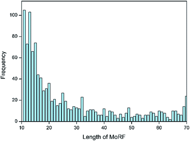
Following the approach of Mohan et al.,10 an initial dataset of MoRFs was constructed from the June 2015 version of the Protein Data Bank (PDB)21 by selecting MoRF regions between 10 and 70 residues, which interact with other protein chains greater than 100 residues. Analysis on the lengths for all MoRFs showed that approximately two-thirds of the selected chains had lengths between 10 and 25 residues, as illustrated by Fig. 1. In most other existing methods, e.g. the works of Disfani et al.,16 Fang et al.17 and Nawar Malhis et al.,19 only the short MoRF regions with 5–25 residues were considered in their datasets. However, there are still a large number of MoRFs (the remaining one-third) had lengths between 26 and 70 residues that cannot be ignored. Hence, in this paper, a comprehensive dataset of MoRFs with the widest length between 10 to 70 residues were constructed. Our choice for selecting protein chains with lengths less than 70 residues stemmed from the fact that such short protein chains would be less likely to form a rigid three-dimensional structure prior to interaction. However, on the other hand, protein fragments shorter than 10 residues were not considered in our dataset, mainly in order to facilitate mapping MoRF chains to their parent sequences, because many MoRF chains in PDB are relatively small fragments of longer proteins and such short peptides could not be long enough to match the parent protein sequences. Also, using 10 as a lower bound can reduce the chance of mingling chameleon segments,22 the longest of which so far observed are 8 residues in length.23Initially, we used the PDB advanced search in order to isolate entries containing more than 2 protein entities and at least one sequence between 10 and 70 residues which is a putative MoRF. Using these two criteria, a dataset consisting of 6966 protein complexes was assembled and the corresponding PDB files were downloaded to obtain sequences. The first step was to remove nucleotide sequences and chains with ambiguous sequence information (i.e., sequence containing X or Z annotations instead of real amino acids) from our initial dataset. After that, only the 2987 containing at least one protein sequence longer than 100 residues were used from the remaining PDB entries. The cutoff at 100 amino acids was chosen to avoid discarding shorter folded domains. The next step was to remove sequence redundancy by CD-Hit24 with default parameters and sequence identity cutoff at 30%. Then 1957 chains were remained. These remaining MoRFs were mapped to the UniProtKB/Swiss-Prot and as a result, 1103 MoRF segments were successfully mapped to their parent sequences and in the remaining cases the MoRFs were too short to uniquely map to the UniProt or could not be found. The amino acids that form these MoRFs were annotated in the parent sequences and these sequences were used to develop and assess our predictor. The detailed information of this dataset is shown in the ESI file S1.† We divided the dataset into training and testing sets according to the ratio of 9![[thin space (1/6-em)]](https://www.rsc.org/images/entities/char_2009.gif) :
:![[thin space (1/6-em)]](https://www.rsc.org/images/entities/char_2009.gif) 1. Finally, the non-redundant training and independent test datasets have 993 and 110 chains, respectively. The training dataset was used to construct and valid the SVM models and the test dataset was used to evaluate our method.
1. Finally, the non-redundant training and independent test datasets have 993 and 110 chains, respectively. The training dataset was used to construct and valid the SVM models and the test dataset was used to evaluate our method.
All previous MoRFs predictors used the annotated MoRF regions in the training set as the positive samples and all the remaining residues in these chains (all residues except those that compose MoRFs) were by default assumed as negative samples. However, since MoRF regions are defined as small segments in a larger segment of disorder, the sequence surrounding a given MoRF region within longer intrinsically disordered regions is less likely to contain unannotated MoRFs, compared to the remaining parts that are far away from the known MoRFs of the chain.16 That is to say, some of the non-MoRFs in fact will be proved the MoRFs because the current MoRF annotations available are incomplete. Moreover, the negative dataset constructed in this way is so extremely huge, but only a tiny proportion of them are used to validate the prediction model. So the prediction results may be biased on the different negative samples.
In this work, we first extracted a large window from the intrinsically disordered regions that contain a given MoRF. So the 20 flanking amino acids on each side of the MoRF that we call flanking region was used as the negative samples. In this way, we can effectively avoid many possible false negatives in the datasets to some extent. In the end, our training dataset has 14![[thin space (1/6-em)]](https://www.rsc.org/images/entities/char_2009.gif) 080 residues. All positive samples (7040 MoRFs residues) and an equal number of randomly selected negative samples (7040 non-MoRFs residues) from original set were used to train our prediction model.
080 residues. All positive samples (7040 MoRFs residues) and an equal number of randomly selected negative samples (7040 non-MoRFs residues) from original set were used to train our prediction model.
2.2 Feature extraction and selection
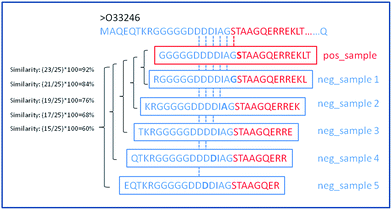
In this work, three types of features were used to formulate the biological samples with an effective mathematical expression that can truly reflect their intrinsic correlation with the target to be predicted. The total number of considered features is 172. For each residue in a given input chain, we try to incorporate the information about the residue itself and its neighbors. To do so, we create a sliding window of size 25 that is centered on the input residue and we extract information from this window to calculate the feature set. Fig. 2 shows the schematic diagram of sliding window strategy. For the residues on both termini (ends) of the sequence where there are no neighbouring residues on the right or left side, we fill these positions with default values. Calculations of the features for each position in the window was inspired by the previous methods, α-MoRF-PredI11 and α-MoRF-PredII,13 which are used to predict disorder and secondary structure.From Fig. 2, for a given protein sequence, we can see that the way we extract negative samples would result in high sequence similarity between the MoRFs and the flanking regions (non-MoRFs) with the highest sequence identity of 92%. It makes more difficult to distinguish whether a given residue belongs to a MoRFs or not for a predictor, although the flanking regions are less likely to contain unannotated MoRFs and the false negatives could be effectively avoided. However, on the other hand, it can be concluded that if we could distinguish the MoRFs from the flanking regions, the MoRFs and other real non-MoRFs far away from the known MoRFs could be easily classified.
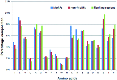 | ||
| Fig. 3 Distributions of AAC in three regions of MoRF regions (blue), 20-residue long flanking regions (green) and non-MoRF regions (red), respectively. | ||
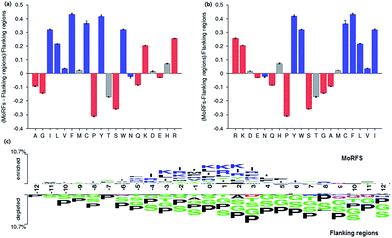
The AAC of MoRFs is different from that of the general protein population and contrasts most with the sequences flanking them, which agrees with the results of Disfani et al.,16 Nawar Malhis et al.18 and Mészáros et al.25 Therefore, AAC is a useful feature to represent the sequence information of MoRF regions. It was computed to evaluate the number of occurrences of 20 amino acids normalized with total number of residues in a protein. It is defined as:
 | (1) |
For a query protein sequence, we first find its K nearest neighbors in both positive and negative sets according to local sequence similarity. For example, for two local sequence fragments S1 and S2 (the window size is 2n + 1), define the distance D(S1,S2) between S1 and S2 as:
 | (2) |
 | (3) |
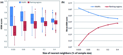
KNN scores measure the evolutionary similarity of the local sequence surrounding a query site between positive set and negative set. A score greater than 0.5 means the query site is more similar to the positive samples and a score smaller than 0.5 means it is more similar to the negative samples. The larger the KNN score is, the more similar the fragment is to some known MoRFs, and thus, the more likely it is a MoRF. Fig. 5 compares the KNN scores of MoRFs with those of the flanking regions. Overall, MoRFs have higher scores than flanking regions. The average KNN scores with different sizes of nearest neighbors are within 0.52–0.69 for MoRFs. Therefore, after excluding self-matches, as expected, the local sequences surrounding known MoRFs are more similar to their nearest neighbors in positive set. For flanking regions, the KNN scores are within 0.10–0.45, which means that the sequences in negative set are more similar to nearest neighbors in negative set. As displayed in Fig. 5, with the increasing of the value of K, the gap of KNN scores between MoRFs and the flanking regions is getting smaller and smaller, which is consistent with the theory of KNN. Through testing, when K was chosen to be 0.025%, 0.05%, 0.1%, 0.2% and 0.4% of the size of the training set, the predictive result reached its maximum. In short, the KNN scores capture evolutionary similarity information in the local sequence around MoRFs and hence distinguish them from the background. Therefore, KNN scores are suitable as features for MoRFs prediction.
2.3 Feature importance evaluation
Although three different types of descriptors (20 + 147 + 5) were obtained, these 172 attributes in the feature set are not equally relevant to the MoRFs prediction. In order to evaluate the contribution of each variable, four feature selection approaches, including CorrelationAttributeEval, GainRatioAttributeEval, OneRAttributeEval and ReliefAttributeEval were used to rank the 172 attributes. CorrelationAttributeEval29 evaluates the worth of an attribute by measuring the Pearson's correlation between it and the class. Nominal attributes are considered on a value by value basis by treating each value as an indicator. An overall correlation for a nominal attribute is arrived at via a weighted average. GainRatioAttributeEval29 evaluates the attributes by measuring the gain ratio with respect to the class. OneRAttributeEval29 selects attributes based on the oneR classifier. OneR (also called 1R) is a very simple and convenient program which classifies examples on the basis of a single attribute and can be used to describe the structure of the data. ReliefAttributeEval29 can operate on both discrete and continuous class data. It ranks the features by repeatedly sampling an instance and considering the value of the given attribute for the nearest instance of the same or different class. In this work, these feature processes were performed by WEKA (3.7.10).292.4 Performance evaluation
Prediction of MoRFs is performed for each amino acid in the input chain. The evaluation criteria follow the work in Disfani et al. The evaluation criteria include accuracy, true-positive rate (TPR), false-positive rate (FPR) and the area under the receiver operating characteristic (ROC) curve (AUC). These metrics are defined as follows:
 | (4) |
 | (5) |
 | (6) |
In our study, support vector machine (SVM) was used to identify whether a given residue belongs to a MoRFs or not. SVM is considered as one of the most accurate machine learning algorithms and has been frequently used to address classification problems in bioinformatics, such as secondary structure prediction,30 protein fold recognition31 and protein–protein interaction.32
For the actual implementation, LIBSVM package33 was used and a Radial Basis Function (RBF) was chosen as the kernel function. In order to maximize the performance of the SVM algorithm, the optimal set of parameters, the penalty parameter c and the kernel width parameter g, were then optimized using a grid search approach. We consider c = 2x and g = 2x, where x = −8, −7, …, 7, 8.
To train and construct a SVM model, 5-fold cross-validation tests was performed. The training dataset are randomly divided into five groups. Each group in turn is used as a testing set, and the remaining four groups are merged to train the SVM model. The average performance of 5 times is the final results of 5-fold cross-validation tests.
3. Result and discussion
3.1 Selection of the most representative SVM model
In order to get the optimal features, four feature selection methods were used to evaluate the 172 attributes for the training dataset. Afterwards, the importance score of each feature variable was obtained by each feature selection method. From the rank list of the importance scores, the top 15, 25, 35, 45 or 55 features were respectively selected for each feature selection method. In this way, 20 (5 × 4) feature sets were obtained by the four feature selection methods.Finally, 100 (20 × 5) SVM models were developed by five-fold cross validation test. We mapped the performance of each model to the square chart, where Se is the x-axis and Sp is the y-axis, as shown in Fig. 6. Among the 100 models, we can see that models constructed with features selected method by ReliefAttributeEval give the relatively high and balanced Sp and Se. So we further shorten the interval of feature sets in order to select the best feature set. The top 20, 30, 40 or 50 features were respectively selected according to the rank list of the importance scores and hence we constructed another 20 (4 × 5) models. By 5-fold cross-validation, the average performance of the corresponding 9 models constructed with features selected by ReliefAttributeEval with the top 15, 20, 25, 30, 35, 40, 45, 50 and 55 features is respectively shown in Fig. 7. In the end, we totally constructed 120 (100 + 20) models.
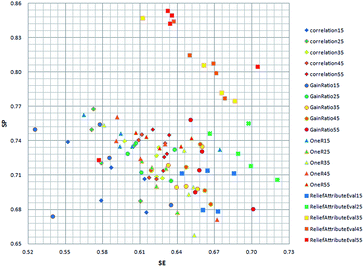 | ||
| Fig. 6 Distribution of the Se and Sp with different model by different feature selection method and different number of feature set. | ||
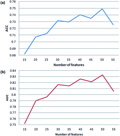 | ||
| Fig. 7 Cross-validation accuracy and AUC of our method based on feature sets with different number of variables. | ||
We can know that the most representative model includes 50 optimal features selected by ReliefAttributeEval (WEKA (3.7.10)) (see detail information of ranked attributes in the ESI file S2†) and it results in a satisfactory performance in the prediction quality reflected by the accuracy of 75.75% and AUC of 0.8368, so we used this set of features to construct the final prediction model. Compared to the number of features (50), the amount of samples (14![[thin space (1/6-em)]](https://www.rsc.org/images/entities/char_2009.gif) 080) in the training set is also enough to cover all the sample space.
080) in the training set is also enough to cover all the sample space.
Among these 50 optimal features, all 5 KNN score features are included in this optimal feature set and the top 3 are all KNN score features. As for CTD features, there are 37 out of 147 CTD features relevant to hydrophobicity, normalized van der Waals volume, polarizability, secondary structures and solvent accessibility in this optimal feature set. As we know, MoRFs are rich in hydrophobic residues and the polar residues, while the flanking regions are depleted in hydrophobic residues and polar residues so they might have significant difference on these properties. At last, there are 8 out of 20 AAC features in this optimal feature set and they represent the composition of Leu, Val, Phe, Arg, Ile, Lys, Ser and Met, respectively. Fig. 3 shows that the composition difference of these amino acid between the MoRFs and the flanking regions is more significant than other amino acids. In conclusion, these selected features are appropriate and effective for characterizing the MoRFs.
3.2 Results on the independent test dataset
We evaluated the practical performance of our model with an independent test set of 110 protein sequences, including 2978 MoRF residues and 87![[thin space (1/6-em)]](https://www.rsc.org/images/entities/char_2009.gif) 362 non-MoRF residues that include 3484 flanking residues and 83
362 non-MoRF residues that include 3484 flanking residues and 83![[thin space (1/6-em)]](https://www.rsc.org/images/entities/char_2009.gif) 878 non-flanking residues. The result proves that our method by only considering flanking regions rather than all other residues except MoRF residues as negative samples has yielded a promising performance with a total accuracy of 64.98% and AUC of 0.5223 on the test set. Detailed results can be seen in Table 1. The sequence similarities between the MoRFs and other non-MoRFs far away from the known MoRFs are lower than those between the MoRFs and flanking regions, the prediction accuracy of the model on the non-MoRF and flanking residues should be higher than that of the model on flanking residues. However, we can observe that the model gives an accuracy of 65.66% on the non-flanking residues, which is slightly lower than that of the model on flanking residues (70.41%). The reason may be that there are certain unknown MoRFs in the non-MoRF and flanking residues, so these false negatives are predicted as MoRFs and these samples are misclassified by our model for the current available annotation information. We believe that with more unknown MoRFs being discovered in the near future, these false negatives will be testified by our method.
878 non-flanking residues. The result proves that our method by only considering flanking regions rather than all other residues except MoRF residues as negative samples has yielded a promising performance with a total accuracy of 64.98% and AUC of 0.5223 on the test set. Detailed results can be seen in Table 1. The sequence similarities between the MoRFs and other non-MoRFs far away from the known MoRFs are lower than those between the MoRFs and flanking regions, the prediction accuracy of the model on the non-MoRF and flanking residues should be higher than that of the model on flanking residues. However, we can observe that the model gives an accuracy of 65.66% on the non-flanking residues, which is slightly lower than that of the model on flanking residues (70.41%). The reason may be that there are certain unknown MoRFs in the non-MoRF and flanking residues, so these false negatives are predicted as MoRFs and these samples are misclassified by our model for the current available annotation information. We believe that with more unknown MoRFs being discovered in the near future, these false negatives will be testified by our method.
| Test dataset | ACC | TPR | FPR | AUC |
|---|---|---|---|---|
| MoRFs residues | 0.3942 | 0.3942 | — | — |
| Flanking residues | 0.7041 | — | 0.2959 | — |
| Non-flanking residues | 0.6566 | — | 0.3434 | — |
| Total | 0.6498 | 0.3942 | 0.3415 | 0.5223 |
3.3 Justification of the negative samples defining methods
In previous studies,16,17,19 only the short MoRF regions with 5–25 residues were considered in their dataset. Since there have not been the experimentally confirmed non-MoRF residues available, by excluding the annotated MoRF regions in as the positive samples, all the remaining residues in these chains were by default assumed as negative samples in these reports. However, we constructed a comprehensive dataset of MoRFs with a large length of 10–70 residues and only the residues in flanking regions were used the negative samples. To confirm the effectiveness of our new way of defining negative samples and to determine how it might benefit the prediction, two testes were implemented here.First, we run our method with the new way of defining negative samples on shorter MoRFs which are only 5–25 amino acids in other previous studies. It would answer the question whether our new way of defining negative samples increases performance on known data sets. Based on our training dataset, it results in a good performance with the accuracy of 92.85% and AUC of 0.9679 by 5-fold cross-validation. Detailed results can be seen in Table S2 of the ESI file S3.† The results show that by using our way of defining negative samples on the training dataset, the prediction performance increases significantly on known data sets, which could demonstrate that our new way of defining negative samples can benefit the MoRF prediction.
On the other hand, we also run our method with the old way of defining negative samples (as in other predictors) on longer MoRFs which are 10–70 amino acids as in the dataset of our work. This test would validate our approach to choosing the MoRF dataset. Based on the training dataset, it also results in a satisfactory performance with the accuracy of 73.58% and AUC of 0.8016 by 5-fold cross-validation. Detailed results can also be seen in Table S3 of the ESI file S3.† For comparison, we also provide detailed information about the results of our method with the new way of defining negative samples on the dataset of 10–70 amino acids MoRFs. Detailed results can be seen in Table S4 of ESI file S3.† With the new way of defining negative samples in our work, the performance of our method is better than that of the old way of defining negative samples on the dataset of our work. These results demonstrate that our approach to choosing the new MoRF dataset is more effective.
In addition, since the first test shares a common independent test dataset with our work, we have also run this test on the this same independent test dataset. Detailed results of the prediction performance of this test on the independent test dataset can be seen in Table S5 of ESI file S3.† By comprising Table S5† with Table 1 in Section 3.2, we can see that the TPR value 0.3942 of our work is about 10% higher than that (TPR value 0.3042) of the old way of defining negative samples. However, since our method is relatively poor in identifying the negative sample than that of the old way of defining negative samples, the AUC value 0.5223 of our method is also relatively lower than that (AUC value 0.6417) of the old way of defining negative samples.
3.4 External validation on the negative samples
In order to further demonstrate the prediction specificity of our method, an additional independent test dataset called NEGATIVE which sourced from Disfani et al.16 was constructed. It includes 28 proteins that are likely to have no MoRFs. Meanwhile comparisons were performed between our representative model and other three previously published methods including ANCHOR, MoRFpred and MoRFCHiBi_web which are available via web servers on negative samples. ANCHOR is a web-based implementation of an original method that takes a single amino acid sequence as an input and predicts protein binding regions that are disordered in isolation but can undergo disorder-to-order transition upon binding. The server combines the general disorder tendency with the sensitivity to the structural environment. MoRFpred is a comprehensive predictor which combines the annotations generated by sequence alignments with the prediction results generated by SVM. Table 2 lists the prediction results of the four methods on negative samples. As we can see, our method and all these three predictors achieved good performance. Among them, our method performed best and all negative samples were correctly predicted. On the other hand, 43 negatives samples were misclassified by ANCHOR, 550 by MoRFpred and 465 by MoRFCHiBi_web.| Dataset | Method | ACC | TPR | FPR | AUC |
|---|---|---|---|---|---|
| NEGATIVE | Our method | 1.0000 | — | 0.0000 | — |
| ANCHOR | 0.9953 | — | 0.0047 | — | |
| MoRFpred | 0.9403 | — | 0.0597 | — | |
| MoRFCHiBi_web | 0.9495 | — | 0.0505 | — |
3.5 Case studies
Two case studies were used to further demonstrate the predictive ability of our method. They were selected from EXPER2008-12 dataset collected by Disfani et al.16 that includes proteins with MoRFs in regions that were experimentally verified to be disordered in isolation. The first case concerns a short native MoRF segment, while the second concerns a long segment. The shortest MoRF and the longest MoRF in EXPER2008-12 are 9 and 23 residues respectively.The first case study is the 274 residues long Septin-4 protein (Uiprot ID: O43236-6). The native MoRF region in this protein is located at the C-termini and is 9 residues long. Fig. 8a shows that the native MoRF region in this protein is located from 266 to 274 residues and our approach has predicted three potential MoRFs located from 1 to 4 residues, 231 to 233 residues and 268 to 274 residues, respectively. Among them, the third predicted MoRF region is almost completely overlap to the native MoRF region, indicating our method has predicted 7 residues out of 9 residues which consist of a MoRF region.
The second one is Antitoxin phd protein (Uiprot ID: Q06253). It has 73 residues and contains a MoRF region which is 23 residues long. Fig. 8b shows that the native MoRF region in this protein is located from 51 to 73 residues and our approach has predicted two potential MoRFs located from 3 to 5 residues and 61–71 residues. As a result, our predictor has predicted 11 residues out of 23 residues that consist of a MoRF region. Besides the annotated MoRF regions can be detected by our method, other unknown regions (residues) were also predicted as the potential MoRF regions that are needed to be confirmed by the experimental methods.
In addition, we also have compared our method to ANCHOR, MoRFpred and MoRFCHiBi_web using this known data set called EXPER2008-12. The comparison results are listed in Table S6 of the ESI file S3.† Our method results in a satisfactory performance in the prediction quality reflected by the accuracy of 88.46% and AUC of 0.6350 and it gives the best ACC and the lowest FPR among these methods.
4. Conclusions
The aim of this study is to develop a reliable method to identify the location of the MoRFs. Here, we proposed a new sequence-based predictor of MoRFs. Rigorous model construction and testing was implemented. First, a comprehensive dataset was constructed to establish statistical predictors by collecting protein sequences with MoRFs of length between 10 to 70 residues. Second, we developed a new way to define the negative samples by using the 20 flanking amino acids on each side of the MoRF region as the negative samples. Then, we used AAC and two previously unexplored features including CTD and KNN scores as features to characterize sequence information. Finally, through the feature selection, the final representative SVM model was selected and achieved a comparative performance with other existing methods. The case studies show that our method can practically identify MoRFs with a promising result.Acknowledgements
This work was funded by the National Natural Science Foundation of China (No. 21675114, 21573151).References
- R. V. D. Lee, M. Buljan, B. Lang, R. J. Weatheritt, G. W. Daughdrill and A. K. Dunker, et al., Chem. Rev., 2014, 114, 6589–6631 CrossRef PubMed.
- C. J. Oldfield and A. K. Dunker, Annu. Rev. Biochem., 2014, 83, 553–584 CrossRef CAS PubMed.
- P. E. Wright and H. J. Dyson, Nat. Rev. Mol. Cell Biol., 2015, 16, 18–29 CrossRef CAS PubMed.
- V. N. Uversky, C. J. Oldfield and A. K. Dunker, J. Mol. Recognit., 2005, 18, 343–384 CrossRef CAS PubMed.
- A. K. Dunker and Z. Obradovic, Nat. Biotechnol., 2001, 19, 805–806 CrossRef CAS PubMed.
- A. K. Dunker, Z. Obradovic, P. Romero, E. C. Garner and C. J. Brown, Genome. Inform. Ser. Workshop Genome. Inform., 2000, 11, 161–171 CAS.
- J. J. Ward, J. S. Sodhi, L. J. Mcguffin, B. F. Buxton and D. T. Jones, J. Mol. Biol., 2004, 337, 635–645 CrossRef CAS PubMed.
- C. J. Oldfield, Y. Cheng, M. S. Cortese, C. J. Brown, V. N. Uversky and A. K. Dunker, Biochem., 2005, 44, 1989–2000 CrossRef CAS PubMed.
- A. Cumberworth, G. Lamour, M. M. Babu and J. Gsponer, Biochem. J., 2013, 454, 361–369 CrossRef CAS PubMed.
- A. Mohan, C. J. Oldfield, P. Radivojac, V. Vacic, M. S. Cortese, A. K. Dunker and V. N. Uversky, J. Mol. Biol., 2006, 362, 1043–1059 CrossRef CAS PubMed.
- C. J. Oldfield, Y. Cheng, M. S. Cortese, P. Romero, V. N. Uversky and A. K. Dunker, Biochemistry, 2005, 44, 12454–12470 CrossRef CAS PubMed.
- V. Vacic, C. J. Oldfield, A. Mohan, P. Radivojac, M. S. Cortese, V. N. Uversky and A. K. Dunker, J. Proteome Res., 2007, 6, 2351–2366 CrossRef CAS PubMed.
- Y. Cheng, C. J. Oldfield, J. Meng, P. Romero, V. N. Uversky and A. K. Dunker, Biochemistry, 2007, 46, 13468–13477 CrossRef CAS PubMed.
- M. M. Babu, R. V. D. Lee, N. S. D. Groot and J. Gsponer, Curr. Opin. Struct. Biol., 2011, 21, 432–440 CrossRef CAS PubMed.
- Z. Dosztányi, B. Mészáros and I. Simon, Bioinformatics, 2009, 25, 2745–2746 CrossRef PubMed.
- F. M. Disfani, W. L. Hsu, M. J. Mizianty, C. J. Oldfield, B. Xue, A. K. Dunker, V. N. Uversky and L. kurgan, Bioinformatics, 2012, 28, 75–83 CrossRef PubMed.
- C. Fang, T. Noguchi, D. Tominaga and H. Yamana, BMC Bioinf., 2013, 14, 1–14 CrossRef PubMed.
- N. Malhis and R. J. Gsponer, Bioinformatics, 2015, 31, 1738–1744 CrossRef CAS PubMed.
- N. Malhis, E. T. Wong, R. Nassar and J. Gsponer, PLoS One, 2015, 10, e0141603 Search PubMed.
- I. Walsh, A. J. Martin, D. T. Di and S. C. Tosatto, Bioinformatics, 2012, 28, 503–509 CrossRef CAS PubMed.
- H. Berman, K. Henrick, H. Nakamura and J. L. Markley, Nucleic Acids Res., 2007, 35, 301–303 CrossRef PubMed.
- M. D. Jr and P. S. Kim, Nature, 1996, 380, 730–734 CrossRef PubMed.
- I. Jacoboni, P. L. Martelli, P. Fariselli, M. Compiani and R. Casadio, Proteins, 2000, 41, 535–544 CrossRef CAS.
- Y. Huang, B. Niu, Y. Gao, L. Fu and W. Li, Bioinformatics, 2010, 26, 680–682 CrossRef CAS PubMed.
- B. Mészáros, I. Simon and Z. Dosztányi, PLoS Comput. Biol., 2009, 5(5), 819–833 Search PubMed.
- H. B. Shen, J. Yang and K. C. Chou, J. Theor. Biol., 2006, 240, 9–13 CrossRef CAS PubMed.
- S. Tan, Expert Syst. Appl., 2006, 30, 290–298 CrossRef.
- J. Gao, J. J. Thelen, A. K. Dunker and D. Xu, Mol. Cell. Proteomics, 2010, 9, 2586–2600 CAS.
- B. M. Hall, E. Frank, G. Holmes, B. Pfahringer, P. Reutemann and I. H. Witten, ACM SIGKDD Explorations Newsletter, 2009, 11, 10–18 CrossRef.
- S. Hua and Z. Sun, J. Mol. Biol., 2001, 308, 397–407 CrossRef CAS PubMed.
- C. H. Q. Ding and I. Dubchak, Bioinformatics, 2001, 17, 349–358 CrossRef CAS PubMed.
- M. Rashid, S. Ramasamy and G. P. Raghava, Curr. Protein Pept. Sci., 2010, 11, 589–600 CrossRef CAS PubMed.
- C. C. Chang and C. J. Lin, ACM Transactions on Intelligent Systems and Technology, 2011, 2, 389–396 CrossRef.
Footnote |
| † Electronic supplementary information (ESI) available. See DOI: 10.1039/c6ra27161h |
| This journal is © The Royal Society of Chemistry 2017 |

