
 Open Access Article
 This Open Access Article is licensed under a
 Creative Commons Attribution 3.0 Unported Licence
Understanding surface interactions in aqueous miscible organic solvent treated layered double hydroxides
Valentina Erastova *a,
Matteo T. Degiacomib,
Dermot O'Hareb and
H. Chris Greenwell*a
*a,
Matteo T. Degiacomib,
Dermot O'Hareb and
H. Chris Greenwell*a
aDepartment of Earth Sciences, Durham University, South Road, Durham DH1 3LE, UK. E-mail: valentina.erastova@durham.ac.uk; chris.greenwell@durham.ac.uk
bChemistry Research Laboratory, Department of Chemistry, University of Oxford, 12 Mansfield Road, Oxford, OX1 3TA, UK
First published on 20th December 2016
Abstract
Layered materials are of interest for use in a wealth of technological applications, many of which require a high surface area for optimal properties and performance. Recently, an industrially scalable method to create high surface area layered double hydroxide (LDH) materials, which may be readily dispersed in non-polar solvents, has been developed. This method involves treatment of LDHs with aqueous miscible organic (AMO) solvents. Here, molecular modeling is exploited to elucidate the AMO solvent–LDH interactions, in order to understand how the dispersion process is facilitated by the AMO treatment. The simulations show how hydrogen-bond networks within the LDH interlayer are disrupted by AMO solvents, leading to delamination.
Introduction
Layered, or lamellar, solids consist of stacks of 2-dimensional inorganic/organic layers, where intralayer bonding is strong but interlayer bonding is weak. Such materials are of great interest in a number of technology areas including adsorbents,1 catalysts and catalyst precursors,2 nanocomposite materials3,4 and novel battery materials,5 amongst others. For many of these applications a high surface area is desirable and this can be achieved via exfoliating and dispersion of the 2-dimensional sheets in a suitable liquid. Layered double hydroxides (LDHs) are a class of ionic lamellar compounds made up of positively charged brucite (Mg(OH)2)-like layers and an interlayer region containing charge-balancing anions and intercalated water. The chemical composition of LDHs can vary, but the most widely encountered class of these materials can be most commonly represented by the formula [M1−xz+Mxy+(OH)2]a+(Xn−)a/n·mH2O, where z = 1 or 2 and y = 3 or 4. Though found naturally as mineral forms in a relatively narrow range of compositions, unlike many other layered minerals, such as the aluminosilicate clays, LDHs may be readily synthesized. In recent years LDHs have garnered a lot of attention owing to their highly tunable composition and morphology for use in catalysis,6 CO2 capture,7,8 drug delivery hosts,9,10 fire retardants,11,12 and cement additives.13,14Despite their utility, owing to strong interlayer bonding networks LDHs suffer from a drawback in terms of the ease at which a high surface area materials may be attained. As such, numerous studies have been carried out to develop methods for delamination of LDHs. These studies, inspired by the early work of Hibino,15,16 have tended to focus on intercalating reactive monomer/solvent combinations, which facilitate the disruption of the ionic interactions between the LDH layers. A drawback of such approaches is the necessity for specific anions, often organic, to be intercalated into the LDH interlayer prior to the delamination process. Such processes invariably require the LDH synthesis to be completed under an inert atmosphere, to avoid atmospheric carbon dioxide intercalating as carbonate into the LDH, favoured by the typically high pH of LDH synthesis. Carbonate has a very high affinity for the LDH layer, relative to ions with lower charge density, which results in extremely high inter-sheet binding.
However, in a sequence of recent work an aqueous miscible organic solvent treatment (AMOST) has been successfully used to disperse chloride, borate, nitrate, sulfate and carbonate LDHs, and termed the resultant materials AMO–LDHs.17–19 AMO–LDH carbonate materials have the generalized formula [M1−xz+Mxy+(OH)2]a+(CO3)a/2·mH2O × n(AMO-solvent), they exhibit very large N2 Brunauer–Emmett–Teller (BET) surface areas, pore volumes, low powder densities and may be readily dispersed in non-polar solvents. For example, these compounds have been show to exhibit N2 BET surface areas ∼400 m2 g−1, in comparison to ∼1–100 m2 g−1 for conventionally prepared carbonate-intercalated LDHs. The mechanism by which the AMOST approach facilitates a large surface area is not yet fully understood. Critically, the AMOST method works for carbonate intercalated LDHs and is extremely facile in its application. In order to optimize the AMOST, an understanding and, ideally, quantification of the effect of the solvent on the water-treated LDH is required.
In order to study the interlayer regions and surfaces of nano-materials such as layered minerals, computer simulations have become an essential adjunct to experimental methods, offering understanding of the reactivity, structure and dynamics of interfacial regions at an atomistic and molecular level. Molecular dynamics (MD) simulations, in particular, allow reproduction of conditions and data analogous to experimental conditions; they are stochastic and allow systems to evolve according to given temperatures and pressures. MD simulations have been successfully used to study LDH materials, especially with respect to surface bonding, dynamics of interlayer species and materials properties.20–22
In order to elucidate the mechanism behind the AMOST process, in this present work MD simulations are used to study Mg6Al2(OH)16CO3 – LDHs as a function of the ratio of water to AMO solvent, to replicate the gradual replacement of water during the experimental repeated washing process. In this study successful aqueous miscible organic (AMO) solvents18 are investigated: acetone, dimethyl sulfoxide, dioxane, ethanol, ethylene glycol, iso-propanol, and tetrahydrofuran. After characterising the mode of action of the above solvents, we also study tert-butanol, to see whether this may be a potentially effective solvent for AMOST. To provide a distinct contrast we also modelled a known non-polar, non-miscible solvent – chloroform. The study delivers an atomistic view of AMOST, simulating the AMO–LDH interactions prior to delamination, providing insights for future optimisation of the experimental process.
Methodology
LDH model
In order to run a MD simulation, an atomistic model of the system of interest must be built. Here we use a unit of LDH with the stoichiometry [Mg3Al(OH)8]+, creating one positive charge per unit cell, counterbalanced by 0.5 carbonate ions. In order to simulate a reasonably large model system and to avoid self-interaction artefacts, the unit cell was replicated in a 5 by 6 array, creating a 3.82 nm by 2.75 nm LDH surface. The LDH layer thickness is 0.53 nm and the layer occupies the region between z = 0 and 0.55 nm. A simulation box was obtained by adding 4 nm of vacuum above the surface.Solvents
The vacuum described above was filled with different solvents to create solvated LDH surfaces. A system containing pure water (WAT) was simulated. Three different systems containing 1400, 1000 and 800 water molecules were run. Water-solvent mixtures to model step wise washing with solvent were also set up as follows: 100 solvent to 1000 water molecules (1![[thin space (1/6-em)]](https://www.rsc.org/images/entities/char_2009.gif) :10 ratio); 200 solvent to 600 water molecules (1:3 ratio) and 300 solvent to 300 water molecules (1:1 ratio). The solvent was varied between acetone (ACT), dimethyl sulfoxide (DMSO), dioxane (DiOx), ethanol (ETH), ethylene glycol (EG), iso-propanol (iP), tert-butanol (tBut), tetrahydrofuran (THF) and chloroform (CHL). Table 1 summarises the properties of the solvents used.
:10 ratio); 200 solvent to 600 water molecules (1:3 ratio) and 300 solvent to 300 water molecules (1:1 ratio). The solvent was varied between acetone (ACT), dimethyl sulfoxide (DMSO), dioxane (DiOx), ethanol (ETH), ethylene glycol (EG), iso-propanol (iP), tert-butanol (tBut), tetrahydrofuran (THF) and chloroform (CHL). Table 1 summarises the properties of the solvents used.
| Solvent | Structure | Density, g mL−1 25 °C | Formula weight, g mol−1 | CDL c-axisa, Å |
|---|---|---|---|---|
| a Crystalline domain length, along solvated LDH c-axis, it taken from data reported in Yang et al.18 | ||||
| Water (WAT) |  |
1.00 | 18.02 | 217.0 |
| Acetone (ACT) |  |
0.791 | 58.08 | 127.3 |
| Dioxane (DiOx) |  |
1.034 | 88.11 | 138.5 |
| Dimethyl sulfoxide (DMSO) |  |
1.100 | 78.13 | 126.6 |
| Ethanol (ETH) |  |
0.789 | 46.07 | 135.8 |
| Ethylene glycol (EG) |  |
1.113 | 90.12 | 130.6 |
| iso-Propanol (iP) |  |
0.785 | 60.10 | 104.4 |
| tert-Butanol (tBut) |  |
0.775 | 74.12 | N/A |
| Terahydrofuran (THF) |  |
0.889 | 72.11 | 122.5 |
| Chloroform (CHL) |  |
1.492 | 119.38 | N/A |
Force field parameters
The ClayFF force field,23 was used to model the LDH within the simulations. This force field is specifically developed to model clay-like minerals, including LDH. The charges were adjusted to create a net positive +1 per unit cell, as described in an earlier paper by the authors.22 The CHARMM36 force field24,25 was used to model the organic solvents and the force field parameters were assigned via the CGenFF algorithm.26 Parameters for chloroform are not included in the original CHARMM force field and therefore were taken from Vorobyov et al.27 ClayFF has been tested previously and used by the present authors with the CHARMM force field.28,29 Both force fields are parameterized for use with SPC water, used in this work.Simulations
The simulations were performed with GROMACS 4.6.7.30,31 Periodic boundary conditions coupled with a large supercell were used to avoid finite size effects. Each simulation was first energy minimized using a steepest descent algorithm with convergence criterion being the maximum force on any one atom to be less than 100 kJ mol−1 nm−1. The system was then equilibrated for 0.5 ns in the isothermal–isobaric (NPT) ensemble with a velocity-rescale Berendsen thermostat set at 300 K and the temperature coupling constant set to 0.1 ps. A semi-isotropic Berendsen barostat was used, set at 1 bar, with a pressure-coupling constant of 1 ps. The minimization and equilibration simulations were run with real-space particle-mesh-Ewald (PME) electrostatics and a van der Waals cutoff of 1.2 nm. After equilibration, a production run of 20 ns was performed. This was run with PME electrostatics and a van der Waals cutoff of 1.4 nm in NPT ensemble, with the same parameters as in the equilibration.Visualization
The snapshots were produced with VMD 1.9.2 32 and the atoms where rendered with the following color scheme: Mg atoms pink, Al cyan, O red, H white, C gray, S in yellow and Cl blue. Due to system periodicity, the same LDH layer visually appears on both sides of the box.Analysis
The density, basal interlayer d-spacing and partial density analysis were performed with GROMACS tools. H-bond analysis was developed and performed with a VMD TCL script, where an H-bond was defined to be at a maximum distance of 3.5 Å between the hydrogen donor and acceptor, and at a maximum angle of 30° between the donor–hydrogen–acceptor. H-bonds were counted using a 1 Å sliding window moving along the z-axis with 0.25 Å steps. The vectorial analysis was developed in-house. A vector between two selected atoms is assigned, shown in Table 1, and defined for each species as follows: acetone – from carbonyl carbon to oxygen; dioxane – two mirror image vectors between oxygens; DMSO – between sulphur and oxygen; ethanol – between the alpha-carbon and the alcohol O; ethylene glycol – a sum of two mirror image vectors between carbon and adjacent oxygens; iso-propyl alcohol – between the alcohol group C and O; tert-butanol – between the alpha-carbon and the alcohol O; THF – from the centre between carbons to the opposing oxygen; and chloroform between carbon and hydrogen. For every solvent molecule, the elevation of its vector with respect of the LDH surface was calculated. Elevations were then collected using a sliding window, as for the H-bond analysis. All data analysis was carried out over the last 10 ns of simulation. For AMO solvents, the partial density, H-bond density and vectorial analysis were plotted only up to 1.8 nm from the surface for clarity, as the solvent properties were no longer influenced by the surface beyond 1.5 nm distance. All data was plotted with Matplotlib.33Results
The modelled systems have solvent in the interlayer domain. Fig. 1A shows a system with the LDH counter-balanced with carbonate and intercalated with water and acetone. The system behaviour is mirrored across the middle of the interlayer separation. The water molecules can be seen concentrating near the surface, forming a hydration layer at the LDH sheet interface, and mixing with acetone molecules further from the surface. Carbonate ions sit close to the LDH surface, within the first water layer. This behaviour is general and can be observed for all AMO solvents. In contrast (Fig. 1B), chloroform separates from both the hydrophilic LDH hydroxide interface and the water forming a pure chloroform layer in the centre of the box. Due to the low miscibility of chloroform and water, such behaviour is to be expected. As such, chloroform simulations correctly act as a negative control. | ||
| Fig. 1 Examples of simulation systems containing LDH (large spheres, periodically represented on both sides of the simulation box), counterbalancing carbonate ions at the surface (thick lines), water and 100 solvent molecules. (A) Acetone mixes with water, while (B) chloroform forms a separate layer. | ||
Change of interlayer spacing and system density as a function of solvent concentration
Fig. 2 shows the dependence of layer d-spacing and system density as a function of the nature of the intercalated solvent. The d-spacing is determined by the volume occupied by intercalated molecules, and so depends on the total number and type of atoms in the system, their intermolecular interactions and compressibility. The total density is determined by the summation of the very dense LDH sheets, and small number of carbonate counter ions, and varying amounts of water and solvents. As a consequence, addition of more interlayer water (light blue line) increases the d-spacing and decreases the total density. A similar trend and slope is shown by slightly heavier dioxane (1.033) and slightly lighter THF (0.889). Note that the lighter solvents will sit to the left of the water trend. tert-Butanol, iso-propanol, acetone and ethanol have even lower specific gravities (0.79–0.78). Therefore, substituting water with these solvents also leads to a reduction of density. Ethylene glycol, DMSO and chloroform are denser than water, so show opposite trends. The systems with the biggest change of the d-spacing vs. density show near-linear increase; while systems where change is smaller show an irregular trend. This phenomenon is strictly driven by an uneven increase in the ratio of only two (solvent:water) out of four components, with the constant fraction of heavier LDH.
 | ||
| Fig. 2 The d-spacing as a function of total density for solvents and water. 100 solvent molecules are shown with a circle, 200 molecules with a triangle and 300 molecules with a square. In the case of water circle is 800 water molecules, triangle – 1000, square – 1400. Errors correspond to the simulation box fluctuations are always below 0.07% and therefore not shown. | ||
Partial density of systems
Fig. 3 shows the partial density of components of the pure water LDH–carbonate system plotted along the z-axis. The simulation box is periodic, therefore the LDH layer is positioned between 0 and 0.3 nm and between 4.3 nm and 4.5 nm. The highest peak corresponds to the metal layer, neighbouring peaks to the oxygen and hydrogen layers, respectively. The LDH layer is not fixed and can therefore fluctuate, leading to occasional widening of the distributions. The water forms three hydration layers near the LDH surface. The first hydration layer is the highest peak at 0.45 nm, i.e. 0.15 nm away from the LDH surface. The second and third hydration layers are at 0.65 nm and 1 nm, respectively. Beyond this distance water displays bulk properties. Carbonate ions are always positioned within the first hydration layer. Fig. 4 shows partial densities for all of the solvent systems. At low solvent concentrations, the AMO solvent molecules mix with water in the bulk region of the box, while chloroform fully separates into a layer. With increase of the AMO-solvent to water ratios the partial density of the solvent in bulk region increases. At higher concentrations the non-cyclic AMO-solvent replaces the third hydration layer and forms a small peak in the density plots at 0.9 nm. The solvent also mixes into the second hydration layer of water, slightly reducing its partial density. At the highest concentration the non-cyclic solvent occupies regions closer to the LDH layer, further decreasing the partial density of remaining water hydration layers. Solvents always localize slightly further than carbonate ions from the LDH surface. All of the non-cyclic AMO-solvents, but tert-butanol, forms a shoulder in the density plots into the 1st hydration layer. DMSO even at 200-concentration, shows mixing into the 1st hydration shell. The effect is further enhanced at highest 300-concentration, where DMSO is strongly present within the 1st hydration shell. Cyclic dioxane and THF do not locate near the surface. At longer range, solvent partial densities show slight ordering, most pronounced in the case of ethylene glycol and DMSO. Chloroform, being non-miscible with water, shows a different behaviour from all other solvents, forming a layer in the centre with a denser edge. With increased solvent ratios the layer thickness grows, while its partial density remains constant and equivalent to pure chloroform (simulated value 1380 kg m−3 at 300 K, experimental value 1465 kg m−3 at 298 K). | ||
| Fig. 3 Partial density of water system showing the location of LDH, carbonate ions and water. LDH distribution appears on both sides of the box, due to system periodicity. Carbonate adsorbs on LDH surface, while water forms three hydration layers. | ||
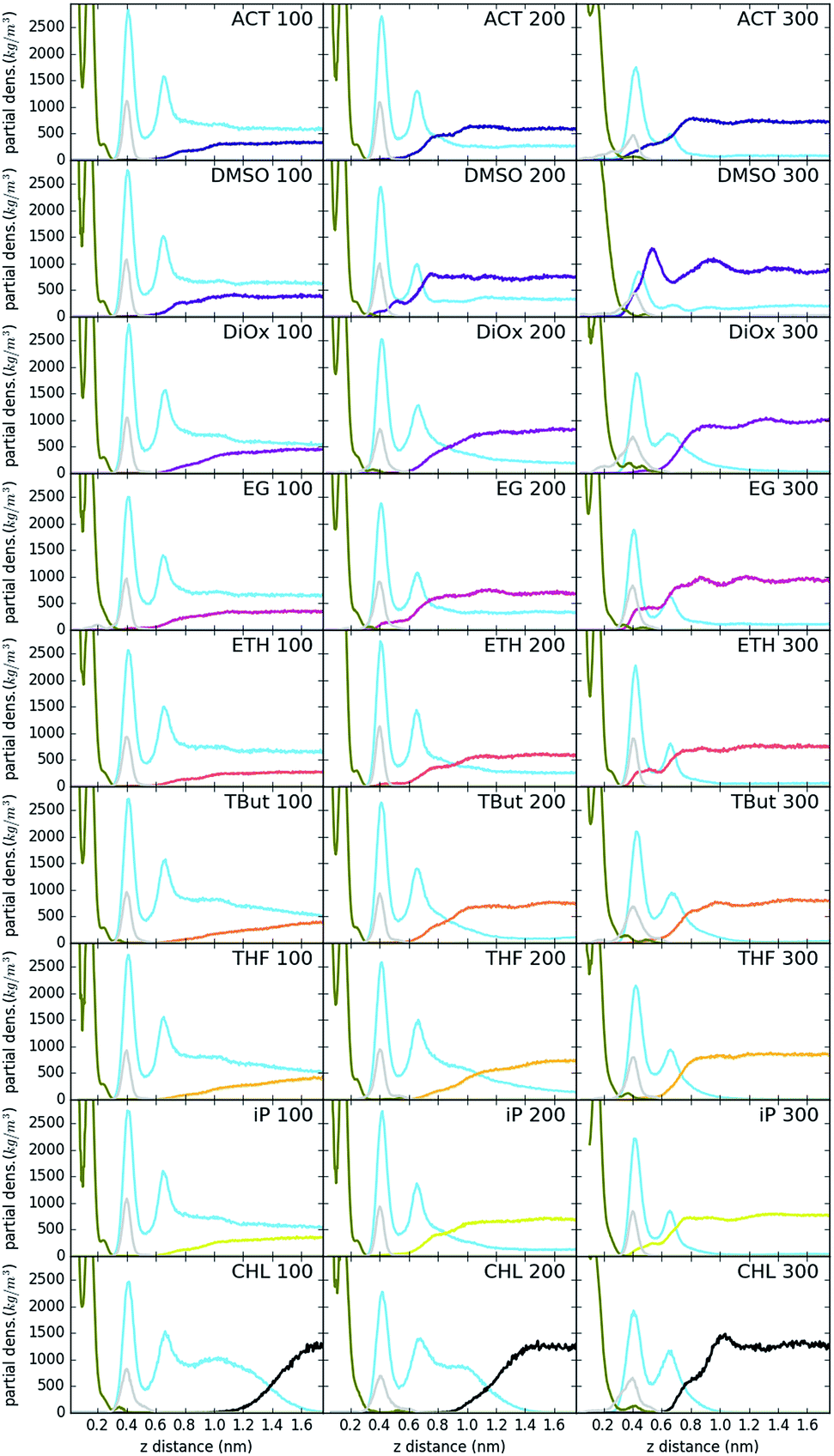 | ||
| Fig. 4 System partial densities for LDH (olive), carbonate (gray), water (light blue) and solvent (other colour). The plots are labelled by solvent name and number of solvent molecules. To correct for simulation-specific fluctuations, datasets are realigned so that the peak of carbonate ion distribution is located at 0.4 nm. | ||
Change of hydrogen-bond density with solvent
Fig. 5 and 6 show the density of H-bonds in both pure water and water–solvent systems. H-bonds arise from all interactions of water, solvent, carbonate and the surface. The number of H-bonds is calculated within a sliding window; it is therefore solely dependent on the local amount of molecules and their packing. Since H-bonds in the pure water system are mostly from water self-interactions, the H-bond distribution resembles the water density profile on Fig. 3. It should, however, be noted that the H-bond peaks are not at the same position as partial density distribution ones. The first peak in the H-bond distribution (at 0.4 nm, Fig. 5) corresponds to the interaction of water and carbonate with the LDH surface, while the second one (0.6 nm, Fig. 5) represents the interaction between the first and second hydration layer. When increasing solvents concentrations, Fig. 6, the number of H-bonds is always significantly reduced. Reduction in the amount of H-bonds between the two adjacent inner hydration layers becomes apparent only at high AMO concentrations. A decrease in the amount of H-bond is also observed in the bulk, with greater effects caused by iso-propanol and ethyl acetate, followed by acetone. DMSO shows greatest H-bond reduction within the 1st hydration shell, while at longer distances the number of H-bonds is not as affected. As expected for a non-AMO solvent, chloroform does not show any structured H-bonding within the chloroform only region. | ||
| Fig. 5 H-bond distribution of the pure water system. The first peak corresponds to interactions with LDH, the second indicates interactions between the first and second hydration layer. | ||
 | ||
| Fig. 6 H-bond distribution across the LDH interlayer systems with solvents. To correct for simulation-specific fluctuations, datasets are realigned so that the first peak is located at 0.4. The plots are labelled by solvent name, while lines show different number of solvent molecules. | ||
Solvent alignment
Fig. 7 shows the relationship of the solvent molecules' alignment with respect to their distance from the LDH surface. Near the surface, all of the AMO solvents have their molecules mostly aligned with their C–O bond at 50–60° relative to the plane of the LDH surface atoms, indicating a direct interaction with the –OH groups of the LDH. Carbonyl/sulfoxide groups interact with the surface via their oxygen. This binding mode allows the molecule to rotate along the C/S![[double bond, length as m-dash]](https://www.rsc.org/images/entities/char_e001.gif) O axis, as well as pivot. In the case of alcohol hydroxyl groups, pivoting and rotation are hindered by the presence of a hydrogen atom. As a consequence, the latter binding allows a narrower range of surface alignment angles. This difference can be observed when comparing acetone (binding via carbonyl) to iso-propanol (binding via hydroxyl).
O axis, as well as pivot. In the case of alcohol hydroxyl groups, pivoting and rotation are hindered by the presence of a hydrogen atom. As a consequence, the latter binding allows a narrower range of surface alignment angles. This difference can be observed when comparing acetone (binding via carbonyl) to iso-propanol (binding via hydroxyl).
 | ||
| Fig. 7 (A) elevation of a vector assigned to the organic solvents as a function of distance from the surface for 300 solvent systems only. (B) Examples showing alignment of solvent molecules on the surface of the LDH at 300 solvent to 300 water mixture: ACT, DMSO, DiOx, EG, ETH, tBut, THF, iP, and CHL. For clarity carbonate is not shown. | ||
EG has a symmetrical OH group on each side of the molecule. For this molecule, two symmetrical alignment vectors were defined. Independently, these –OH groups would interact with the surface like ETH. This is visible as a similar alignment pattern between 0 and 90°. When one –OH group interacts with the surface, the second is oriented away from it. This is expressed in our vectorial analysis by a mirror angle (0 to −90°) located further away from the surface. The OH groups located away from the surface can form favourable H-bonding with the OH groups of other ethylene glycol molecules. This templating effect causes ethylene glycol to feature more distinct patterns in both its density and H-bond profiles.
The cyclic AMO solvents, dioxane and THF, cannot access within a close proximity to the LDH surface, forming an aligned layer beyond the 1st hydration shell. Dioxane has two opposing oxygens that, alike EG, show a symmetrically opposed pattern.
Chloroform shows a very different pattern, as it separates from the water coating the LDH. The slight alignment around 45° at 1 nm away from the surface is due to the chloroform layer exposing its hydrogens oriented towards the water molecules.
Discussion and conclusions
LDH layers maintain their stacking via a network of interlayer bonds. At close distance layers are held together by bridging carbonate ions. Our simulations indicate that, when swollen, the interlayer features a strong network of hydrogen bonds between the interlayer water molecules, and the hydroxyl groups of the LDH sheets. Water forms three hydration layers next to the LDH surface, with carbonate ions located within the first one. We observe that the addition of AMO solvents disrupts this network in a concentration-dependent fashion. At low concentrations solvents localise in the bulk region, behind the second hydration layer. With higher concentrations, AMO solvent distributions feature a small peak behind the second hydration layer. Furthermore, AMOs begin mixing into the second, and then first hydration layer. At highest concentrations, adsorption of non-cyclic AMOs onto the LDH surface was observed. All the AMO solvent species studied feature a specific alignment, indicating a strong interaction with the surface. As a consequence, AMOs' non-polar region orient away from the surface, weakening the H-bond network between the first and second hydration layer.Accordingly, the performance of AMO solvents, adjusted by H-bond count reduction, as presented in the last column of Table 1, show the most effective is iso-propanol, followed by THF, DMSO, acetone, ethylene glycol, ethanol and dioxane. In light of this study the performance is determined by three factors:
1. Capacity of solvent – water mixing. Small, water-miscible solvents are able to adsorb closely onto LDH, accessing the space between first and second hydration layers. This behavior is not expected to be d-spacing dependent, when at least 2 hydration layers are present.
2. Solvent geometry and orientation with respect to LDH layer. When adsorbed a successful AMO solvent should be well aligned and expose its non-polar region to the water. This explains the greater performance of iso-propanol over the more mobile acetone.
3. Efficiency of interfering with the local H-bond network. The bulkier the non-polar region the more effective is the solvent. Even though both iso-propanol and ethanol have same polar group, the latter has less bulky non-polar region and therefore less effective. This also explains why a well-aligned ethylene glycol does not perform as well as iso-propanol. Even though well adsorbed, DMSO shows only moderate increase of performance with respect to acetone as, being highly polar, it is not as good at disrupting the hydrogen bond network.
The effects of tert-butanol in the AMOST process has been investigated though not yet experimentally studied. The solvent aligns well with respect of the mineral surface, exposing the bulky methyl groups and as such is effective in the disruption of the hydrogen bonding network. Nevertheless the bulkiness of these groups does not allow it to access the first hydration shell, limiting its performance. Therefore we predict performance comparable to that of acetone.
As observed by Wang and O'Hare,18 subsequent treatment of the AMO–LDHs may form stable dispersions in non-polar solvent system. The presence of the AMO solvent at the LDH surface would make the LDH layers capable for solvation in non-polar solvents and, as such, help stabilising the particles once dispersed in these solvents. Once solvated, the non-polar solvent should begin to mix into the bulk region and, once there, further disrupt H-bond network. Furthermore, we expect the non-polar solvent to interact with the highly ordered non-polar groups of surface-adsorbed AMOs, contributing to further reducing the H-bond network between the first and second hydration layer. Future work will be dedicated to testing this hypothesis by simulating non-polar solvent systems known to promote AMO–LDH delamination.
Acknowledgements
The authors thank SCG Chemicals Co., Ltd, Thailand for funding this project. The work was carried out using Durham University's high-performance computing services.References
- J. Das, B. S. Patra, N. Baliarsingh and K. M. Parida, Appl. Clay Sci., 2006, 32, 252–260 CrossRef CAS.
- G. Centi and S. Perathoner, Microporous Mesoporous Mater., 2008, 107, 3–15 CrossRef CAS.
- J. N. Coleman, M. Lotya, A. O'Neill, S. D. Bergin, P. J. King, U. Khan, K. Young, A. Gaucher, S. De, R. J. Smith, I. V Shvets, S. K. Arora, G. Stanton, H.-Y. Kim, K. Lee, G. T. Kim, G. S. Duesberg, T. Hallam, J. J. Boland, J. J. Wang, J. F. Donegan, J. C. Grunlan, G. Moriarty, A. Shmeliov, R. J. Nicholls, J. M. Perkins, E. M. Grieveson, K. Theuwissen, D. W. McComb, P. D. Nellist and V. Nicolosi, Science, 2011, 331, 568–571 CrossRef CAS PubMed.
- M. Alexandre and P. Dubois, Mater. Sci. Eng., R, 2000, 28, 1–63 CrossRef.
- J. W. Fergus, J. Power Sources, 2010, 195, 939–954 CrossRef CAS.
- E. Li, Z. P. Xu and V. Rudolph, Appl. Catal., B, 2009, 88, 42–49 CrossRef CAS.
- Q. Wang, J. Luo, Z. Zhong and A. Borgna, Energy Environ. Sci., 2011, 4, 42–55 CAS.
- M. K. R. Reddy, Z. P. Xu, G. Q. M. Lu and J. C. D. Costa, Society, 2006, 45, 7504–7509 Search PubMed.
- J. M. Oh, M. Park, S. T. Kim, J. Y. Jung, Y. G. Kang and J. H. Choy, J. Phys. Chem. Solids, 2006, 67, 1024–1027 CrossRef CAS.
- K. Ladewig, Z. P. Xu and G. Q. M. Lu, Expert Opin. Drug Delivery, 2009, 6, 907–922 CrossRef CAS PubMed.
- A. Edenharter and J. Breu, Appl. Clay Sci., 2015, 114, 603–608 CrossRef CAS.
- M. Zammarano, M. Franceschi, S. Bellayer, J. W. Gilman and S. Meriani, Polymer, 2005, 46, 9314–9328 CrossRef CAS.
- J. D. Mangadlao, P. Cao and R. C. Advincula, J. Pet. Sci. Eng., 2015, 129, 63–76 CrossRef CAS.
- L. Raki, J. Beaudoin, R. Alizadeh, J. Makar and T. Sato, Materials, 2010, 3, 918–942 CrossRef CAS.
- T. Hibino and W. Jones, J. Mater. Chem., 2001, 11, 1321–1323 RSC.
- T. Hibino and M. Kobayashi, J. Mater. Chem., 2005, 15, 653 RSC.
- Q. Wang and D. O'Hare, Chem. Commun., 2013, 49, 6301 RSC.
- M. Yang, O. McDermott, J.-C. Buffet and D. O'Hare, RSC Adv., 2014, 4, 51676–51682 RSC.
- C. Chen, M. Yang, Q. Wang, J.-C. Buffet and D. O'Hare, J. Mater. Chem. A, 2014, 2, 15102 CAS.
- J. Wang, A. G. Kalinichev and R. J. Kirkpatrick, Geochim. Cosmochim. Acta, 2006, 70, 562–582 CrossRef CAS.
- R. T. Cygan, J. a. Greathouse, H. Heinz and A. G. Kalinichev, J. Mater. Chem., 2009, 19, 2470 RSC.
- B. Grégoire, V. Erastova, D. L. Geatches, S. J. Clark, H. C. Greenwell and D. G. Fraser, Geochim. Cosmochim. Acta, 2016, 176, 239–258 CrossRef.
- R. T. Cygan, J.-J. Liang and A. G. Kalinichev, J. Phys. Chem. B, 2004, 108, 1255–1266 CrossRef CAS.
- K. Vanommeslaeghe, E. Hatcher, C. Acharya, S. Kundu, S. Zhong, J. Shim, E. Darian, O. Guvench, P. Lopes, I. Vorobyov and A. D. Mackerell, J. Comput. Chem., 2010, 31, 671–690 CAS.
- E. Lindahl, P. Bjelkmar, P. Larsson, M. A. Cuendet and B. Hess, J. Chem. Theory Comput., 2010, 6, 459–466 CrossRef PubMed.
- K. Vanommeslaeghe and A. D. MacKerell, J. Chem. Inf. Model., 2012, 52, 3144–3154 CrossRef CAS PubMed.
- I. Vorobyov, W. F. D. Bennett, D. P. Tieleman, T. W. Allen and S. Noskov, J. Chem. Theory Comput., 2012, 8, 618–628 CrossRef CAS PubMed.
- T. Underwood, V. Erastova, P. Cubillas and H. C. Greenwell, J. Phys. Chem. C, 2015, 119, 7282–7294 CAS.
- T. Underwood, V. Erastova and H. C. Greenwell, J. Phys. Chem. C, 2016, 120, 11433–11449 CAS.
- D. Van Der Spoel, E. Lindahl, B. Hess, G. Groenhof, A. E. Mark and H. J. C. Berendsen, J. Comput. Chem., 2005, 26, 1701–1718 CrossRef CAS PubMed.
- S. Pronk, S. Páll, R. Schulz, P. Larsson, P. Bjelkmar, R. Apostolov, M. R. Shirts, J. C. Smith, P. M. Kasson, D. Van Der Spoel, B. Hess and E. Lindahl, Bioinformatics, 2013, 29, 845–854 CrossRef CAS PubMed.
- W. Humphrey, A. Dalke and K. Schulten, J. Mol. Graphics, 1996, 14, 33–38 CrossRef CAS PubMed.
- J. D. Hunter, Comput. Sci. Eng., 2007, 9, 99–104 CrossRef.
| This journal is © The Royal Society of Chemistry 2017 |