
 Open Access Article
 This Open Access Article is licensed under a Creative Commons Attribution-Non Commercial 3.0 Unported Licence
Nonlinear intrinsic dissipation in single layer MoS2 resonators
Subhadeep De ,
K. Kunal and
N. R. Aluru*
,
K. Kunal and
N. R. Aluru*
Department of Mechanical Science and Engineering, Beckman Institute for Advanced Science and Technology, University of Illinois at Urbana-Champaign, Urbana, Illinois 61801, USA. E-mail: aluru@illinois.edu
First published on 19th January 2017
Abstract
Using dissipation models based on Akhiezer theory, we analyze the microscopic origin of nonlinearity in intrinsic loss of a single layer MoS2. We study the intrinsic dissipation of single layer MoS2 under axial and flexural mode of deformation using molecular dynamics (MD) simulation. We compare the amplitude scaling of intrinsic dissipation for both the cases with our proposed model. In the axial deformation case, we found a higher (4th) order dependence of dissipation on the strain amplitude. This nonlinearity is shown to stem from the strain dependence of the phonon mode Grüneisen parameter (PMGP) and is accounted for in our dissipation model. In the flexural deformation case, dissipation is found to have a stronger dependence (≥4) on the amplitude of the transverse motion. This nonlinearity can be explained by considering the coupling between out-of-plane motion and in-plane stretching. The proposed model for the flexure deformation case, which accounts for both kinds of nonlinearity, provides a good estimate of dissipation.
I. Introduction
Nanomechanical resonators, based on atomically thin two-dimensional (2D) structures, like graphene and MoS2, have shown intriguing prospects1 in measurement and sensing of fundamental quantities like position, mass, charge2–9 to the level of individual quanta. Extraordinary material properties,10–12 such as high mechanical stiffness and low mass, combined with large surface to volume ratio, have enabled these 2D structures to be potential candidates for high sensitivity measurements. The performance of these nanoresonators is limited by different dissipative mechanisms associated with the vibration mode of operation during the detection process.13,14 For instance, in the case of detection of foreign mass by the shift in resonant frequency of the nanoresonator, a low dissipation ensures better resolution of frequency shift.15,16 Out of different mechanisms that contribute to the dissipation process,17 phonon mediated dissipation dominates at very high frequencies.18 One interesting aspect of damping in 2D structures is its nonlinearity. In the case of graphene resonators, damping is found to be strongly dependent on the amplitude of motion.19 This is explained by introducing a nonlinear damping term (ηx2dx/dt) in the Newton's equation of motion for a harmonic oscillator where η is a constant, x is position and t is time. A theoretical treatment reveals that the nonlinearity emerges from the coupling between flexural modes and the in-plane modes.20 The coupling is due to the geometric effect associated with the flexural motion.21–23 This geometric nonlinearity can manifest itself in phonon interaction and Akhiezer dissipation.24 The effect can be particularly significant when the operational frequency of the flexural motion is of the order of a few gigahertz.Akhiezer damping is a dominant intrinsic loss mechanism for nanoscale resonators operating at gigahertz frequencies.25 This takes place as a result of interaction of mechanical deformation with the modes of thermal vibration, called phonons. An applied strain field can couple with the phonon modes, and thus modulate their frequencies.26,27 The fractional change in phonon frequencies is proportional to the strain. In the case of flexural deformation with fixed boundaries, the out of plane motion may accompany in-plane stretching due to the geometric effect. Consequently, the strain at each section may have a second and higher order dependence on the amplitude of transverse motion. Hence, the coupling between the out-of-plane motion and phonon modes is effectively nonlinear. Though this is a common scenario in the case of flexural deformation of clamped 2D structures like graphene and MoS2, its effect on intrinsic dissipation has not yet been explored. Previous studies have shown that, in the case of graphene, which is one atomic layer thick, the unstable out of plane modes28 and the edge atoms29 play a major role in intrinsic dissipation. But very few studies have been directed towards investigating dissipation in a single layer MoS2.30–32 This work focuses on studying the underlying physics behind intrinsic dissipation of single layer MoS2 using MD simulation. A simplified dissipation model is introduced which is based on the physical mechanism. Using this model, the effect of nonlinearity on intrinsic dissipation is investigated and compared under different modes of deformation.
MD simulations have been previously employed to study intrinsic dissipation in nano-structures.25 Axial deformation of beams at gigahertz frequencies is characterized by a homogeneous strain field. In this case, intrinsic dissipation is explained using Akhiezer theory.33 On the other hand, flexural deformation of thin beams involves a linearly varying strain along the transverse (thickness) direction. This results in thermoelastic damping,34,35 in addition to Akhiezer damping. Flexural deformation of thin 2D structures with fixed boundaries induces a strain field that is different from that in beams. In the membrane limit, the 2D structure provides negligible resistance to bending forces and undergoes stretching along its plane.36 A single layer MoS2 exhibits this behavior and will be an interesting candidate for study of intrinsic dissipation. In this work, we employ MD simulation to study intrinsic dissipation in a single layer MoS2. We first show that the intrinsic dissipation during in-plane straining of a single layer MoS2 can be explained using Akhiezer theory. A simplified dissipation model is developed. This model shows good agreement with frequency and amplitude scaling of dissipation in MoS2 under in-plane deformation. Then, we extend this framework for dissipation under flexural deformation by incorporating the geometric effect. A closed form expression for dissipation under flexural deformation is derived. It has atleast fourth and higher order dependence on the amplitude of transverse motion, which shows that the dissipation is indeed nonlinear. Using this expression, the net intrinsic dissipation during flexure deformation can be accurately estimated.
II. Theory
We consider a single layer MoS2 sheet stretched in the x–y plane. The MoS2 sheet is pre-stretched biaxially such that it has a uniform initial tensile stress σ0. For simplicity, the sheet is assumed to be infinitely long along the y direction by imposing periodic boundary condition. The edges of the two-dimensional (2D) sheet along the x direction are clamped as shown in Fig. 1. The length L0 of the sheet between the two clamped edges undergoes deformation. The dynamics of single layer MoS2 resonators can be described by the continuum theory of 2D membranes.10,12 With this knowledge, we first obtain the displacement and the strain field produced in the MoS2 sheet under axial and flexural excitation. The strain field thus obtained is subsequently used to formulate the dissipation in the structure.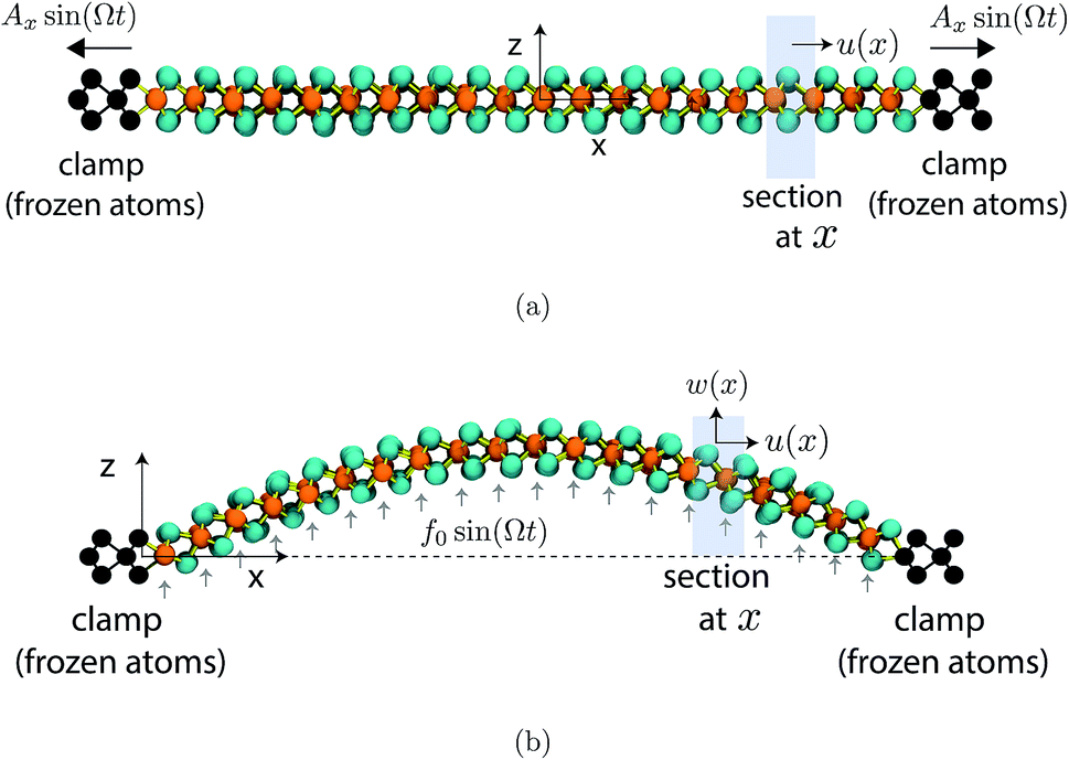 | ||
| Fig. 1 (a) A single layer MoS2 under axial deformation. Ax is the amplitude of displacement of the edge atoms along the x axis. (b) A single layer MoS2 under flexural deformation. A uniformly distributed load with amplitude f0 is applied in the z direction. In both the cases, the clamped edges (frozen atoms) are shown in black. The shaded area shows a section along the length of the MoS2 sheet with the displacement field. | ||
A. Response to periodic excitation
The MoS2 sheet is axially deformed by moving the clamped edges in a periodic manner. The right and the left edge is displaced simultaneously as Ax![[thin space (1/6-em)]](https://www.rsc.org/images/entities/char_2009.gif) sin(Ωt) in the positive and negative x direction respectively, as shown in Fig. 1a. Here Ax is the amplitude of oscillation and Ω is the deformation frequency. Using the results from continuum mechanics, the in-plane displacement field generated in the 2D sheet can be expressed as36
sin(Ωt) in the positive and negative x direction respectively, as shown in Fig. 1a. Here Ax is the amplitude of oscillation and Ω is the deformation frequency. Using the results from continuum mechanics, the in-plane displacement field generated in the 2D sheet can be expressed as36  . Lc denotes a length scale25 given by
  and Am is the amplitude of axial motion which depends on Ax. The angular frequency of oscillation of the fundamental longitudinal mode of the resonator of given length L0 is
  . Considering a deformation frequency much smaller than the fundamental frequency (Ω ≪ ωc) of the resonator would imply Lc ≫ L0. Under this condition, the displacement field along the length of the resonator is approximately linear in
  given by
 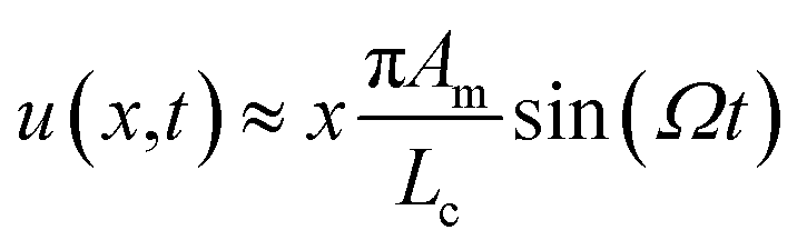 . Further, using the boundary conditions at L0, we can write,
 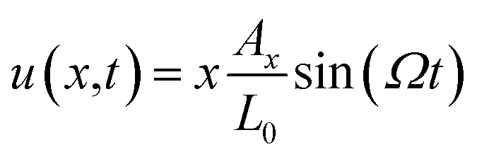 . The linearity in the displacement field results in a spatially uniform strain field in the structure. The periodic strain field can be represented as ε = εasin(Ωt), with the strain amplitude
 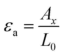 .
.
In case of flexural deformation, the sheet is subjected to a uniformly distributed load f(t) = f0sin(Ωt), in the z direction as shown in Fig. 1b. The resulting displacement field along the x and z direction is denoted by u(x) and w(x) respectively. From continuum theory, the dominant mode shape of deformation due to forcing under the assumed boundary condition is given by36 w(x,t) ∼ Azsin(πx/L0)sin(Ωt) and u(x,t) ∼ 0. Here, Az is the amplitude of flexural motion which depends on f0. Under this mode of deformation, each section along the length of the MoS2 sheet undergoes stretching. The corresponding strain field in the structure is 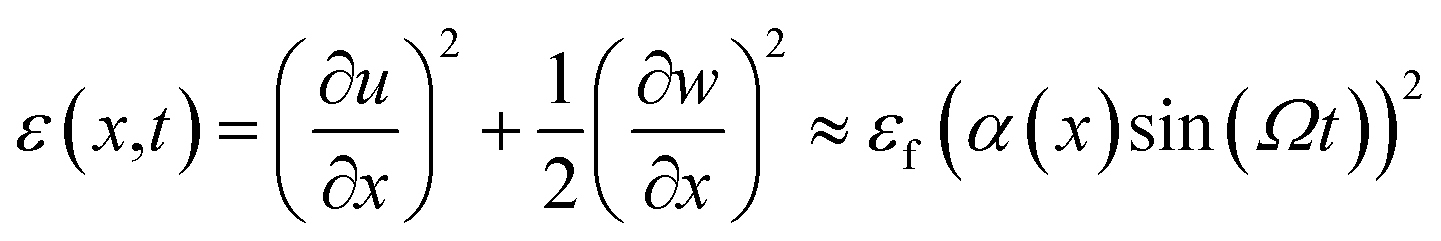 , where
 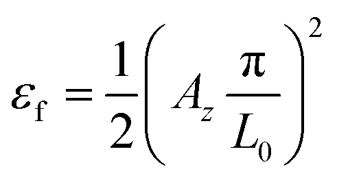 and α(x) = cos(πx/L0). Unlike the axial case, the strain field in the flexure case is non-uniform along the length of the MoS2 sheet. These strain fields serve as an input to calculate the net intrinsic dissipation in the MoS2 sheet under each case of deformation.
B. Formulation of dissipation
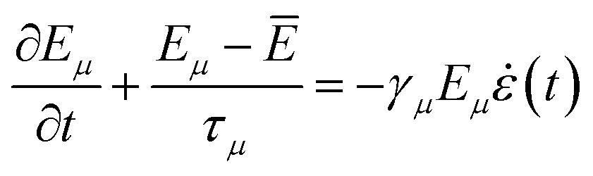
The dissipation due to interaction of the time-varying strain field in a structure with its thermal phonons can be formulated using Akhiezer theory.24 The thermal phonons in the structure share equal energy at thermodynamic equilibrium. On application of strain, the system of phonons is driven out of equilibrium due to the modulation of phonon frequencies. These phonons try to relax back to equilibrium by exchanging energy, which leads to energy loss. We first try to write the equation for evolution of the phonon energies. The energy of each phonon mode at thermodynamic equilibrium, is given by kBT, where kB is the Boltzmann constant and T is the temperature. Any strain, ε can couple with the energy of the phonon mode, Eμ by changing its frequency, ωμ. The coupling factor,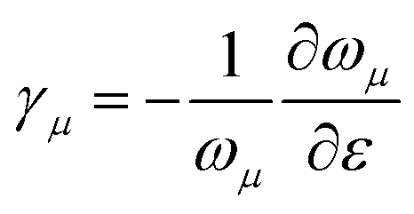 (ref. 37) is defined as the phonon mode Grüneisen parameter (PMGP). For a time varying strain field with frequency Ω, if Ω ≪ ωμ, the ratio Eμ/ωμ is constant.38 Using this and the coupling relation, we can write
 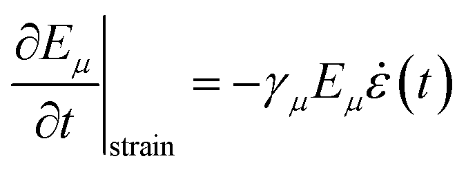 , where (·) denotes derivative with respect to t. Again, the phonon modes can exchange energy due to anharmonic coupling. This coupling governs the relaxation of perturbed energy of the phonon system towards a new equilibrium. Usually each phonon has its own time scale of relaxation,27 τμ. The phonon relaxation mechanism can be approximated as
 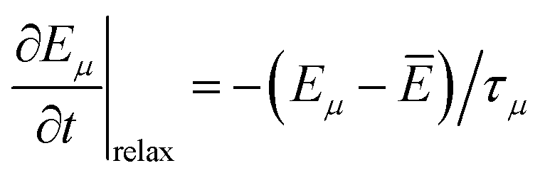 , where Ē is the mean energy of the phonon system at that instant. Thus, the modulation of phonon energies due to straining and relaxation process can be written as
 | (1) |
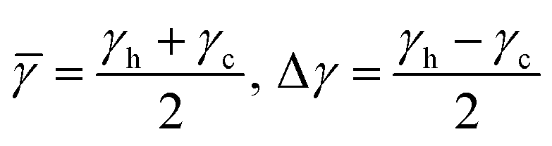
To simplify the system of phonon modes, we employ the phonon grouping technique39 and derive an expression for dissipation. The mean Grüneisen parameter of the ensemble of phonons is defined as  , where N is the total number of phonon modes. The phonon modes with γμ <
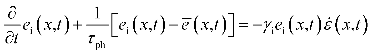
 ![[small gamma, Greek, macron]](https://www.rsc.org/images/entities/i_char_e0c4.gif) constitute the ‘hot’ phonon group and the rest with γμ ≥ constitute the ‘cold’ phonon group. The average Grüneisen parameter of the ‘hot’ phonon group is denoted as γh and that of the ‘cold’ phonon group as γc. During the relaxation process, the energy exchange takes place between the ‘hot’ and ‘cold’ phonon group with a collective relaxation time τph. For a space dependent strain field, ε(x,t), the set of equations governing the energy evolution of the phonon groups at any section of the MoS2 can be expressed as
constitute the ‘hot’ phonon group and the rest with γμ ≥ constitute the ‘cold’ phonon group. The average Grüneisen parameter of the ‘hot’ phonon group is denoted as γh and that of the ‘cold’ phonon group as γc. During the relaxation process, the energy exchange takes place between the ‘hot’ and ‘cold’ phonon group with a collective relaxation time τph. For a space dependent strain field, ε(x,t), the set of equations governing the energy evolution of the phonon groups at any section of the MoS2 can be expressed as
 | (2) |
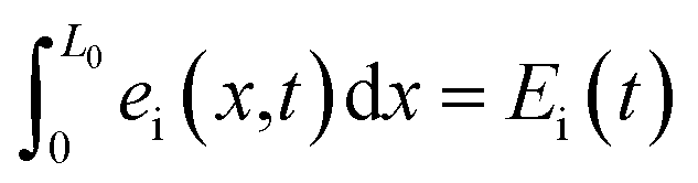 . Here i denotes the ‘hot’ (h) and ‘cold’ (c) phonon group.
  denotes the mean energy of the phonon system at x. Eqn (2) leads to two equations. Adding and subtracting them, we get a set of equations,
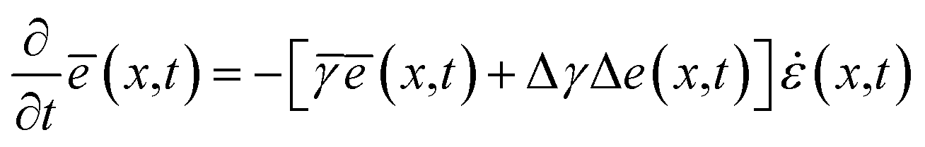 | (3a) |
 | (3b) |
 .
. 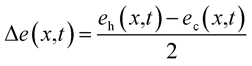 denotes the energy difference between the phonon groups at x. Eqn (3a) and (b) denotes the rate of change of mean energy of the phonon system and the rate of energy exchange between the phonon groups respectively, at any position x. The treatment of energy relaxation in our formulation accounts for the spectral flow energy i.e. flow of energy between different modes. In the case of a spatially inhomogeneous strain field, there also exists a spatial energy gradient given by
  , where (′) denotes derivative with respect to x. The time scale of energy relaxation due to the spatial flow of energy corresponds to the thermal diffusion time34 τtd. In our case, this relaxation mechanism is weak because τtd ≫ 1/Ω and can be ignored. Thus, the energy modulation and redistribution in the structure is microscopically governed by the set of eqn (3a) and (b).
In case of axial deformation, the strain field is found to be spatially uniform i.e. ε(x,t) = εasin(Ωt). The PMGP can be strain dependent if the material behaves nonlinearly.40 Assuming a linear dependence on strain (discussed further in Section IV A), γi can be expressed as γi = γ0i + γ1iε, where γ0i and γ1i are the material constants. Initially, before imparting any deformation, the mean energy of the phonon system satisfies  and the energy difference between the phonon groups satisfy
 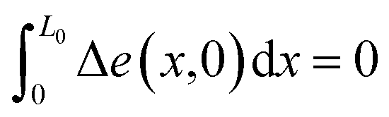 . Considering Δe(x,t) ≪ kBT during the deformation process, ē(x,t) can be approximately solved using the set of eqn (3a) and (b). At steady state, the energy dissipated over the nth period of deformation is given by D = ē(x,Tn+1) − ē(x,Tn), where
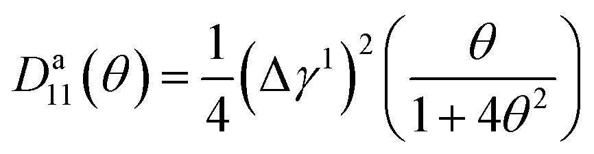
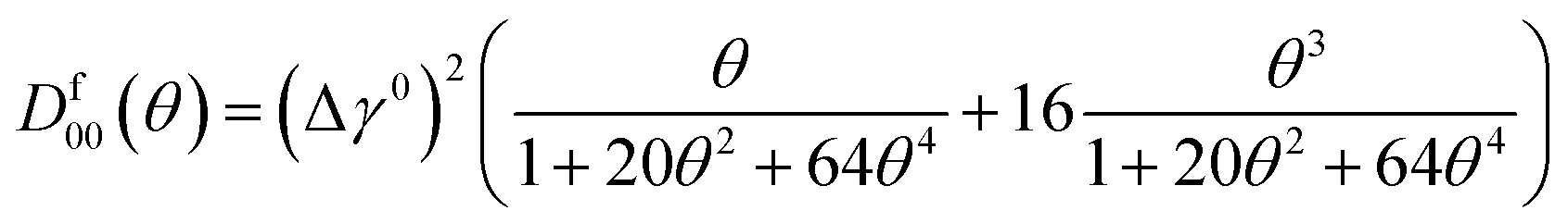
  and Tn = nT. The closed form expression of dissipation, in the axial case, thus obtained, is, Da(x,θ) = πkBT(Da00(θ)εa2 + Da11(θ)εa4)/L0. Here, θ = Ωτph is a metric that determines the strength of the Akhiezer mechanism and
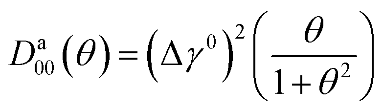
Also,
 . Integrating over the length L0, we get the total dissipation in the structure as
| Eadiss = πkBT(Da00(θ)εa2 + Da11(θ)εa4) | (4) |
The 4th order dependence of dissipation on strain amplitude, as shown in eqn (4), is due to strain dependence of the PMGPs. Later in this study, eqn (4) will be used to compare the frequency and amplitude scaling obtained from MD results.
In the case of flexural deformation, the space dependent strain field, as discussed in Section II A, is given by ε(x,t) = εfα(x)2sin(Ωt)2. The strain dependent PMGPs can then be expressed as γi = γ0i + γ1iε(x,t). The dissipation, which is a function of both position and θ in this case, is obtained as Df(x,θ) = πkBT(Df00(θ)α4(x)εf2 + Df01(θ)α6(x)εf3 + D11(θ)α8(x)εf4)/L0. Here, the θ dependent terms are
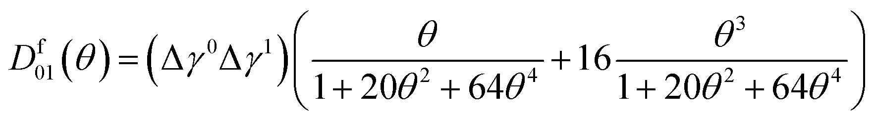
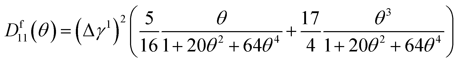
The total dissipation in the structure Efdiss, is obtained by integrating Df(x,Ω) over the length L0. Efdiss is given by
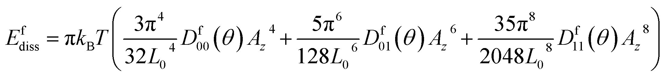 | (5) |
Eqn (5) shows that due to geometric nonlinearity, dissipation during flexure mode of vibration has atleast 4th and higher order dependence in the amplitude of transverse motion. This expression will be used later to estimate dissipation in the flexure case and compare with MD results.
III. Methods
A. Simulation setup
A single layer of MoS2 includes three atomic layers in which a layer of Mo atoms is sandwiched between two layers of S atoms. This geometry (Fig. 1) is initialized and MD simulations are carried out using LAMMPS.41 All visualizations are done using VMD.42 In our MD simulations, the interactions between the Mo–Mo, Mo–S and S–S are modeled using the Stillinger–Weber potential.43 The time step of integration is set to 1 fs for all the simulations. The plane of MoS2 is considered to be along the x–y plane with thickness along the z direction.First, a MoS2 sheet, of dimension 56.16 Å along the x direction and 64.86 Å along the y direction is considered. The sheet is subjected to 5% in-plane pre-straining to prevent any warping or buckling. This is done by scaling the x and the y coordinates of the atoms in the 2D sheet. The pre-stretched sheet is equilibrated to 300 K for 2 ns using Nosé–Hoover thermostat44 with a time constant of 0.1 ps. After equilibration, the structure is further evolved for 2 ns under microcanonical ensemble (with out any thermostat) and atomic trajectories are dumped every 20 fs. The atomic trajectories are used to calculate the PMGPs and energy relaxation time of MoS2 at 300 K.
In order to calculate dissipation under axial mode, the simulation box is deformed along the x direction about its center-of-mass at a given frequency and strain amplitude (shown in Fig. 1a). The structure is evolved under microcanonical ensemble for 100 periods of deformation. The average change of internal energy over the periods of deformation gives a measure of intrinsic dissipation. In the current study, the axial deformation is carried out at frequencies ranging from 5 GHz to 50 GHz at 2% strain amplitude. Dissipation is calculated for strain amplitudes ranging from 1% to 3.5% at 10 GHz.
For the flexural mode of deformation, a MoS2 structure of length 65.68 Å along x direction and 65.01 Å along y direction is considered. The total force on the atoms inside a strip of 5.49 Å at each end along the x direction is set to zero which acts as clamped boundary condition (shown in Fig. 1b). The rest of the atoms are subjected to periodic forcing in the z direction. In our simulations, the forcing frequency is set to 10 GHz and the force applied on each Mo atom of the MoS2 sheet is varied from 0.035 eV Å−1 to 0.046 eV Å−1. The system is evolved under microcanonical ensemble for 100 periods of deformation in order to calculate dissipation.
B. Modal analysis
We perform modal analysis in order to implement the phonon grouping technique and estimate the timescale of energy relaxation. The mode shapes for modal analysis can be obtained using different methods.45 We compute the mode shapes using the results from continuum theory. We, then, use the atomic trajectories from equilibrium MD simulations and FFT technique to calculate the modal frequencies and their dependence on in-plane straining.The allowable in-plane wave vectors can be represented as 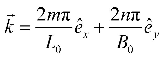 . Here m and n refer to the mode number or order which takes positive integral values. L0 and B0 are the lengths of the MoS2 sheet in the x and y direction with corresponding unit vectors êx and êy respectively. Using linearized membrane theory, the mode shape corresponding to a wave vector
 ![[k with combining right harpoon above (vector)]](https://www.rsc.org/images/entities/i_char_006b_20d1.gif) can be expressed as ϕ(
can be expressed as ϕ(![[r with combining right harpoon above (vector)]](https://www.rsc.org/images/entities/i_char_0072_20d1.gif) ) =
) = ![[P with combining right harpoon above (vector)]](https://www.rsc.org/images/entities/i_char_0050_20d1.gif) exp(j·0), where is the polarization vector and 0 = x0êx + y0êy + z0êz is the mean position vector of the atom. We denote the velocity of the atoms in x, y and z directions as vx, vy and vz. The out-of-plane modal velocities are then given by
exp(j·0), where is the polarization vector and 0 = x0êx + y0êy + z0êz is the mean position vector of the atom. We denote the velocity of the atoms in x, y and z directions as vx, vy and vz. The out-of-plane modal velocities are then given by 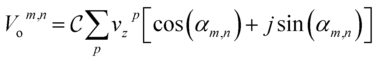 , where
  is the normalizing factor. p sums over all the atoms in the structure. The in-plane modal velocities can be approximated as
  . Using the atomic velocities from MD, the time series of Vom,n(t), Vi-xm,n(t), Vi-ym,n(t) can be computed for different values of m and n. By taking FFT of the auto-correlation of these time series data, the frequencies ωm,n for different modes can be resolved. If the structure is plane strained along the x direction, these frequencies are subject to change. The PMGPs can be estimated46 as
 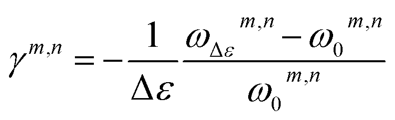 . Here, the subscript 0 and Δε represent the reference and the strained configuration, respectively. The frequencies ωΔεm,n can be calculated for different values of Δε in order to obtain strain dependence of the PMGPs. The PMGPs, then, can be used to perform the phonon grouping.
IV. Results and discussions
A. PMGP and relaxation time
We consider few lower order modes (long wavelength) and calculate the out-of-plane PMGPs (γo) and in-plane PMGPs (γi-x, γi-y) at different magnitude of uniaxial strain. The plot of PMGPs versus strain is shown in Fig. 2. The PMGPs are found to be strain dependent and can be approximated to vary linearly with strain. Similar behavior has been observed for strained monolayer graphene using first principles calculations. It has been shown that under large uniaxial strain, the shifts of the split G mode frequencies depend significantly on the magnitude of the strain.40 Also, the out-of-plane PMGPs are found to be negative and of higher magnitude than in-plane PMGPs (compare Fig. 2c with Fig. 2a and b). This behavior of out-of-plane phonon modes have been addressed in our previous study on graphene nanoribbon.47 From the relation of strain coupling of modal energies (∂E/∂t ∼ ∂T/∂t ∼ −γE![[small epsi, Greek, dot above]](https://www.rsc.org/images/entities/i_char_e0a1.gif) ), we can say that the out-of-plane modes will undergo high positive change in temperature with tensile strain. These modes therefore, primarily constitute the ‘hot’ phonon group. By similar reasoning, looking at the in-plane PMGPs in Fig. 2a and b, we can classify them as the ‘cold’ phonon group. Hence, the relaxation process will involve energy exchange between out-of-plane and in-plane modes.
), we can say that the out-of-plane modes will undergo high positive change in temperature with tensile strain. These modes therefore, primarily constitute the ‘hot’ phonon group. By similar reasoning, looking at the in-plane PMGPs in Fig. 2a and b, we can classify them as the ‘cold’ phonon group. Hence, the relaxation process will involve energy exchange between out-of-plane and in-plane modes.
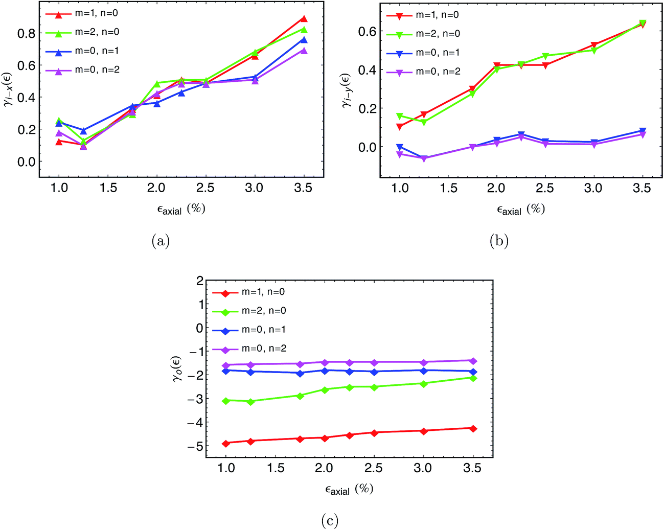 | ||
| Fig. 2 Variation of phonon mode Grüneisen parameters (PMGPs) with axial strain for (a) in-plane modes along the x direction, (b) in-plane modes along the y direction and (c) out-of-plane modes. In the legend, (m,n) indicate the order of the mode. | ||
The time scale of relaxation during the non-equilibrium process can be estimated from the energy fluctuations at equilibrium.48 In this case, fluctuations in total energy of all the out-of-plane modes should be considered. For ease of computation, we deal with the kinetic part of the total energy. Its auto-correlation follows the same decaying behavior as the total energy, but is oscillatory in nature. The total kinetic energy EK of all the out-of-plane modes can be related to the z component of the kinetic energy of each atom as 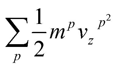 , where p sums over all the atoms. EK(t) is calculated using the atomic trajectories from equilibrium MD simulations for a time length of 2 ns. The normalized auto-correlation of the fluctuations in EK(t) can be computed as
 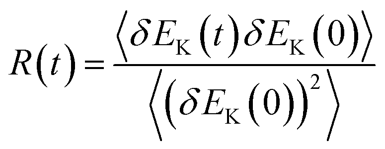 where δEK(t) = EK(t) − 〈EK(t)〉. The envelope of R(t) displays an exponential decay as shown by the solid line in Fig. 3. The timescale of decay, which indicates the energy relaxation time τph can be calculated as
 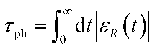 , where εR(t) is the envelope of R(t). In this case τph, is estimated to be 5.24 ps. The τph, thus extracted from the equilibrium MD simulations, serves as direct input to our dissipation model.
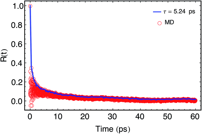 | ||
| Fig. 3 Decay of R(t) with time. The data points corresponding to R(t) are shown by red circles. The solid line is the envelope of R(t) i.e. εR(t). εR(t) is obtained by joining the local peaks of the data points with straight lines. | ||
B. Scaling of dissipation
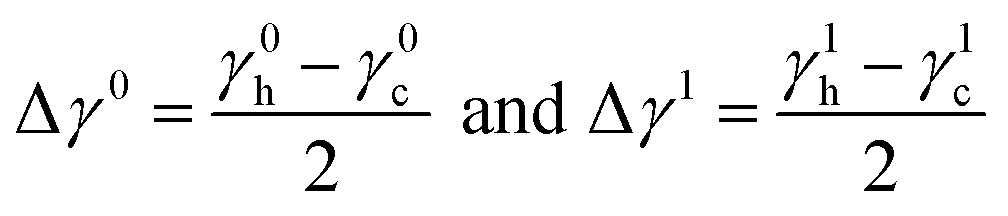
The frequency scaling of dissipation under axial mode of deformation obtained from MD is shown in Fig. 4a. In this case, εa = 0.02 and L0 = 56.18 Å. The Lorentzian nature of the dissipation curve follows directly from the functional form in eqn (4). Using τph as 5.24 ps, a least-square fitting of eqn (4) is performed with the dissipation response. The material parameters, thus evaluated, are |Δγ0| = 0.58 and |Δγ1| = 42.39. Note that |Δγ0| and |Δγ1| here, denote the difference in constant and strain-dependent part of the average PMGPs of out-of-plane (‘hot’ phonon group) and in-plane (‘cold’ phonon group) modes. Thereby, we have the complete set of parameters required for our dissipation models.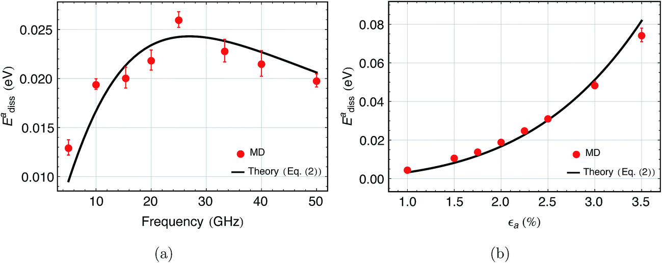 | ||
| Fig. 4 (a) Scaling of dissipation of the single layer MoS2 with frequency of axial deformation at 2% strain. The red circles with error bars correspond to results from MD simulation. The black solid line is the curve-fit using eqn (4). (b) Scaling of dissipation with amplitude of axial strain at 10 GHz. The red circles with error bars correspond to the MD results. The black solid line is the dissipation estimated using eqn (4) as a function of strain. | ||
We, now, try to validate our model for the axial case by comparing the scaling of dissipation with strain amplitude. At Ω = 10 GHz, for εa varying from 1.5% to 3.5%, dissipation obtained using our model (eqn (4)) is in good agreement with the MD results. The comparison is shown in Fig. 4b. The 2nd term in eqn (4), which is 4th order in εa is the nonlinear damping term. At higher strain amplitudes (say εa = 3%), a significant part of the total dissipation (∼55%) is due to nonlinear damping. From eqn (4), it is evident that the relative importance of nonlinear damping depends on |Δγ1εa|. For the cases where |Δγ1εa| ≫ |Δγ0|, the dissipation will be essentially nonlinear.
We, now, look at flexural deformation. Under transverse loading, the deformation profile can be approximated by the fundamental flexural mode and is fitted with Azsin(πx/L0) for Az, where L0 = 54.56 Å. Az increases linearly with the forcing magnitude as shown in Fig. 5a. In the flexure case, Az = 4.47 Å for the maximum forcing considered, which corresponds to a strain amplitude εf = 3.3% close to the edges (x = 0). Taking pre-strain into account, the final state of strain in the structure at any instant is well below the maximum intrinsic strain limit for MoS2.12 Using MD, net dissipation for the structure is obtained for different forcing amplitude at 10 GHz. The plot of dissipation versus Az is shown in Fig. 5b. Inserting the set of previously evaluated parameters in our model for the flexure case (eqn (5)), the estimated dissipation compares well with those obtained from the MD simulation. The lowest order nonlinearity (1st term) in eqn (5) is solely due to the geometric effect which arises from coupling of out-of-plane motion and in-plane stretching. While the last two terms in eqn (5) has the effect of both material and geometric nonlinearity. To get an idea, for flexural deformation with a transverse force which corresponds to Az = 4 Å, the percentage contributions of the 1st, 2nd and 3rd term to total dissipation are ∼29.5%, ∼47.6%, ∼22.8% respectively. The closed form expression for the flexure case shows some interesting behavior. For example, for cases when Δγ0Δγ1 < 0, the 2nd term in eqn (5) has a negative contribution to the total dissipation. Thus, for those cases where the 2nd term is relatively important and negative, it can lead to decrease in dissipation with the increase in Az. It would be useful to identify the cases where this holds true and use it for designing high quality factor nonlinear resonator.
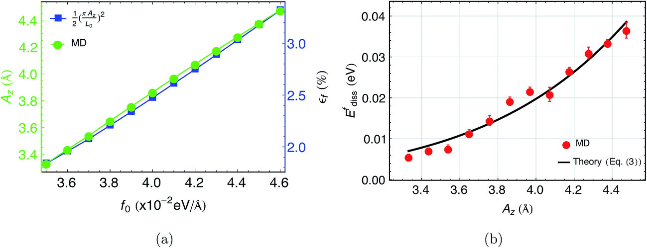 | ||
| Fig. 5 (a) Variation of Az (left axis) and εf (right axis) with transverse loading f0 as obtained from MD simulation. (b) Scaling of dissipation with amplitude of flexural deformation of the single layer MoS2 at 10 GHz. The red circles with error bars correspond to the MD result. The black solid line is the dissipation estimated using eqn (5) as a function of Az. | ||
V. Conclusions
We have studied the microscopic mechanism behind intrinsic dissipation of single layer MoS2. Based on the mechanism, we proposed dissipation models to quantify dissipation under the axial and flexure mode of deformation. We have isolated two factors that renders the dissipation nonlinear: (i) strain dependence of phonon mode Grüneisen (PMGP) and (ii) geometric effect. The later is manifested in the case of flexure deformation because of the coupling between out-of-plane motion and in-plane stretching of MoS2. Our model, which accounts for these factors, can quantify the net dissipation in the flexure case with good accuracy. The developed analytical expressions can be used to engineer high quality factor nanoresonators that operate in the nonlinear regime.Acknowledgements
We gratefully acknowledge the support by NSF under grants 1420882 and 1506619.References
- K. S. Novoselov, V. I. Fal, L. Colombo, P. R. Gellert, M. G. Schwab and K. Kim, A roadmap for graphene, Nature, 2012, 490(7419), 192–200 CrossRef CAS PubMed.
- J. S. Bunch, A. M. Van Der Zande, S. S. Verbridge, I. W. Frank, D. M. Tanenbaum and J. M. Parpia, et al., Electromechanical resonators from graphene sheets, Science, 2007, 315(5811), 490–493 CrossRef CAS PubMed.
- F. Schedin, A. Geim, S. Morozov, E. Hill, P. Blake and M. Katsnelson, et al., Detection of individual gas molecules adsorbed on graphene, Nat. Mater., 2007, 6(9), 652–655 CrossRef CAS PubMed.
- C. Chen, S. Rosenblatt, K. I. Bolotin, W. Kalb, P. Kim and I. Kymissis, et al., Performance of monolayer graphene nanomechanical resonators with electrical readout, Nat. Nanotechnol., 2009, 4(12), 861–867 CrossRef CAS PubMed.
- Y. Dan, Y. Lu, N. J. Kybert, Z. Luo and A. C. Johnson, Intrinsic response of graphene vapor sensors, Nano Lett., 2009, 9(4), 1472–1475 CrossRef CAS PubMed.
- F. K. Perkins, A. L. Friedman, E. Cobas, P. Campbell, G. Jernigan and B. T. Jonker, Chemical vapor sensing with monolayer MoS2, Nano Lett., 2013, 13(2), 668–673 CrossRef CAS PubMed.
- D. J. Late, Y. K. Huang, B. Liu, J. Acharya, S. N. Shirodkar and J. Luo, et al., Sensing behavior of atomically thin-layered MoS2 transistors, ACS Nano, 2013, 7(6), 4879–4891 CrossRef CAS PubMed.
- O. Lopez-Sanchez, D. Lembke, M. Kayci, A. Radenovic and A. Kis, Ultrasensitive photodetectors based on monolayer MoS2, Nat. Nanotechnol., 2013, 8(7), 497–501 CrossRef CAS PubMed.
- C. Zhu, Z. Zeng, H. Li, F. Li, C. Fan and H. Zhang, Single-layer MoS2-based nanoprobes for homogeneous detection of biomolecules, J. Am. Chem. Soc., 2013, 135(16), 5998–6001 CrossRef CAS PubMed.
- A. Castellanos-Gomez, R. van Leeuwen, M. Buscema, H. S. van der Zant, G. A. Steele and W. J. Venstra, Single-Layer MoS2 Mechanical Resonators, Adv. Mater., 2013, 25(46), 6719–6723 CrossRef CAS PubMed.
- S. Bertolazzi, J. Brivio and A. Kis, Stretching and breaking of ultrathin MoS2, ACS Nano, 2011, 5(12), 9703–9709 CrossRef CAS PubMed.
- J. Lee, Z. Wang, K. He, J. Shan and P. X. L. Feng, High frequency MoS2 nanomechanical resonators, ACS Nano, 2013, 7(7), 6086–6091 CrossRef CAS PubMed.
- K. Ekinci and M. Roukes, Nanoelectromechanical systems, Rev. Sci. Instrum., 2005, 76(6), 061101 CrossRef.
- K. Ekinci, Y. Yang and M. Roukes, Ultimate limits to inertial mass sensing based upon nanoelectromechanical systems, J. Appl. Phys., 2004, 95(5), 2682–2689 CrossRef CAS.
- K. Jensen, K. Kim and A. Zettl, An atomic-resolution nanomechanical mass sensor, Nat. Nanotechnol., 2008, 3(9), 533–537 CrossRef CAS PubMed.
- A. Naik, M. Hanay, W. Hiebert, X. Feng and M. Roukes, Towards single-molecule nanomechanical mass spectrometry, Nat. Nanotechnol., 2009, 4(7), 445–450 CrossRef CAS PubMed.
- C. Seoanez, F. Guinea and A. C. Neto, Dissipation in graphene and nanotube resonators, Phys. Rev. B: Condens. Matter Mater. Phys., 2007, 76(12), 125427 CrossRef.
- A. S. Nowick, Anelastic relaxation in crystalline solids, Elsevier, 2012, vol. 1 Search PubMed.
- A. Eichler, J. Moser, J. Chaste, M. Zdrojek, I. Wilson-Rae and A. Bachtold, Nonlinear damping in mechanical resonators made from carbon nanotubes and graphene, Nat. Nanotechnol., 2011, 6(6), 339–342 CrossRef CAS PubMed.
- A. Croy, D. Midtvedt, A. Isacsson and J. M. Kinaret, Nonlinear damping in graphene resonators, Phys. Rev. B: Condens. Matter Mater. Phys., 2012, 86(23), 235435 CrossRef.
- R. Lifshitz and M. Cross, Nonlinear dynamics of nanomechanical and micromechanical resonators, Review of Nonlinear Dynamics and Complexity, 2008, vol. 1, pp. 1–52 Search PubMed.
- M. Imboden, O. Williams and P. Mohanty, Nonlinear dissipation in diamond nanoelectromechanical resonators, Appl. Phys. Lett., 2013, 102(10), 103502 CrossRef.
- M. Imboden, O. A. Williams and P. Mohanty, Observation of nonlinear dissipation in piezoresistive diamond nanomechanical resonators by heterodyne down-mixing, Nano Lett., 2013, 13(9), 4014–4019 CrossRef CAS PubMed.
- A. Akhiezer, J. Phys., 1939, 1, 277 Search PubMed.
- K. Kunal and N. Aluru, Akhiezer damping in nanostructures, Phys. Rev. B: Condens. Matter Mater. Phys., 2011, 84(24), 245450 CrossRef.
- S. S. Iyer and R. N. Candler, Mode- and Direction-Dependent Mechanical Energy Dissipation in Single-Crystal Resonators due to Anharmonic Phonon–Phonon Scattering, Phys. Rev. Appl., 2016, 5(3), 034002 CrossRef.
- J. Turney, E. Landry, A. McGaughey and C. Amon, Predicting phonon properties and thermal conductivity from anharmonic lattice dynamics calculations and molecular dynamics simulations, Phys. Rev. B: Condens. Matter Mater. Phys., 2009, 79(6), 064301 CrossRef.
- K. Kunal and N. Aluru, Intrinsic loss due to unstable modes in graphene, Nanotechnology, 2013, 24(27), 275701 CrossRef CAS PubMed.
- S. Y. Kim and H. S. Park, The importance of edge effects on the intrinsic loss mechanisms of graphene nanoresonators, Nano Lett., 2009, 9(3), 969–974 CrossRef CAS PubMed.
- J. W. Jiang, H. S. Park and T. Rabczuk, MoS2 nanoresonators: intrinsically better than graphene?, Nanoscale, 2014, 6(7), 3618–3625 RSC.
- R. van Leeuwen, A. Castellanos-Gomez, G. Steele, H. van der Zant and W. Venstra, Time-domain response of atomically thin MoS2 nanomechanical resonators, Appl. Phys. Lett., 2014, 105(4), 041911 CrossRef.
- C. Samanta, P. Y. Gangavarapu and A. Naik, Nonlinear mode coupling and internal resonances in MoS2 nanoelectromechanical system, Appl. Phys. Lett., 2015, 107(17), 173110 CrossRef.
- K. Kunal and N. Aluru, Intrinsic dissipation in a nano-mechanical resonator, J. Appl. Phys., 2014, 116(9), 094304 CrossRef.
- R. Lifshitz and M. L. Roukes, Thermoelastic damping in micro- and nanomechanical systems, Phys. Rev. B: Condens. Matter Mater. Phys., 2000, 61(8), 5600 CrossRef CAS.
- S. K. De and N. Aluru, Theory of thermoelastic damping in electrostatically actuated microstructures, Phys. Rev. B: Condens. Matter Mater. Phys., 2006, 74(14), 144305 CrossRef.
- S. S. Rao, Vibration of Membranes, Vibration of Continuous Systems, 2007, pp. 420–456 Search PubMed.
- R. Cowley, The lattice dynamics of an anharmonic crystal, Adv. Phys., 1963, 12(48), 421–480 CrossRef CAS.
- R. M. Kulsrud, Adiabatic invariant of the harmonic oscillator, Phys. Rev., 1957, 106(2), 205 CrossRef.
- S. De, K. Kunal and N. R. Aluru, Mixed role of surface on intrinsic losses in silicon nanostructures, J. Appl. Phys., 2016, 119(11), 114304 CrossRef.
- Y. Cheng, Z. Zhu, G. Huang and U. Schwingenschlögl, Grüneisen parameter of the G mode of strained monolayer graphene, Phys. Rev. B: Condens. Matter Mater. Phys., 2011, 83(11), 115449 CrossRef.
- S. Plimpton, P. Crozier and A. Thompson. LAMMPS-large-scale atomic/molecular massively parallel simulator, Sandia National Laboratories, 2007, vol. 18 Search PubMed.
- W. Humphrey, A. Dalke and K. Schulten, VMD: visual molecular dynamics, J. Mol. Graphics, 1996, 14(1), 33–38 CrossRef CAS PubMed.
- J. W. Jiang, H. S. Park and T. Rabczuk, Molecular dynamics simulations of single-layer molybdenum disulphide (MoS2): Stillinger–Weber parametrization, mechanical properties, and thermal conductivity, J. Appl. Phys., 2013, 114(6), 064307 CrossRef.
- D. J. Evans and B. L. Holian, The Nose–Hoover thermostat, J. Chem. Phys., 1985, 83(8), 4069–4074 CrossRef CAS.
- Z. Tang, H. Zhao, G. Li and N. Aluru, Finite-temperature quasicontinuum method for multiscale analysis of silicon nanostructures, Phys. Rev. B: Condens. Matter Mater. Phys., 2006, 74(6), 064110 CrossRef.
- T. M. G. Mohiuddin, A. Lombardo, R. R. Nair, A. Bonetti, G. Savini and R. Jalil, et al., Uniaxial strain in graphene by Raman spectroscopy: G peak splitting, Grüneisen parameters, and sample orientation, Phys. Rev. B: Condens. Matter Mater. Phys., 2009, 79(20), 205433 CrossRef.
- K. Kunal and N. Aluru, Phonon mediated loss in a graphene nanoribbon, J. Appl. Phys., 2013, 114(8), 084302 CrossRef.
- L. Onsager, Reciprocal relations in irreversible processes. II, Phys. Rev., 1931, 38(12), 2265 CrossRef CAS.
| This journal is © The Royal Society of Chemistry 2017 |