
Elucidating multi-physics interactions in suspensions for the design of polymeric dispersants: a hierarchical machine learning approach†
Aditya
Menon
 a,
Chetali
Gupta
a,
Kedar M.
Perkins
e,
Brian L.
DeCost
a,
Nikita
Budwal
a,
Renee T.
Rios
b,
Kun
Zhang
c,
Barnabás
Póczos
d and
Newell R.
Washburn
*ae
a,
Chetali
Gupta
a,
Kedar M.
Perkins
e,
Brian L.
DeCost
a,
Nikita
Budwal
a,
Renee T.
Rios
b,
Kun
Zhang
c,
Barnabás
Póczos
d and
Newell R.
Washburn
*ae
aDepartment of Materials Science and Engineering, Carnegie Mellon University, Pittsburgh, PA 15213, USA. E-mail: washburn@andrew.cmu.edu; Tel: +1 412 268 2130
bDepartment of Civil and Environmental Engineering, Carnegie Mellon University, Pittsburgh, PA 15213, USA
cDepartment of Philosophy, Carnegie Mellon University, Pittsburgh, PA 15213, USA
dDepartment of Machine Learning, Carnegie Mellon University, Pittsburgh, PA 15213, USA
eDepartment of Chemistry, Carnegie Mellon University, Pittsburgh, PA 15213, USA
First published on 15th June 2017
Abstract
A computational method for understanding and optimizing the properties of complex physical systems is presented using polymeric dispersants as an example. Concentrated suspensions are formulated with dispersants to tune rheological parameters, such as yield stress or viscosity, but their competing effects on solution and particle variables have made it impossible to design them based on our knowledge of the interplay of chemistry and function. Here, physical and statistical modeling are integrated into a hierarchical framework of machine learning that provides insight into sparse experimental datasets. A library of 10 polymers having similar molecular weight but incorporating different functional groups commonly found in aqueous dispersants was used as a training set in magnesium oxide slurries. The compositions of these polymers were the experimental variables that determined the complex system responses, but the method leverages knowledge of the constituent “single-physics” interactions that underlie the suspension properties. Integration of domain knowledge is shown to allow robust predictions based on orders of magnitude fewer samples in the training set compared with purely statistical methods that directly correlate dispersant chemistry with changes in rheological properties. Minimization of the resulting function for slurry yield stress resulted in the prediction of a novel dispersant that was synthesized and shown to impart similar reductions as a leading commercial dispersant but with a significantly different composition and molecular architecture.
Design, System, ApplicationDespite rapid advances in artificial intelligence, most materials for technological applications are still designed using a combination of general physical principles and trial-and-error experimentation due to the complex physical interactions that underlie their performance and the generation of small datasets in research and development. We present a computational method for integrating physical and statistical modeling that provides both insight and properties optimization. The premise of the method is that physical models can be used to augment sparse experimental datasets but an unbiased statistical approach is required to determine how underlying physical forces combine to determine complex system responses. Applied here to the design of polymers for facilitating the flow of particle suspensions, this method required a training set of only 10 polymers (as opposed to 100's or 1000's for purely statistical approaches) to identify a novel dispersant composition whose performance equaled that of the leading commercial material. |
Introduction
Complex physical systems have multiple competing interactions that result in broad spectra of characteristic energy-, length- and timescales, making it challenging to apply computational methods to understand and predict the properties of these systems.1–3 These complicated interactions can also make generating large amounts of data through high-throughput experimentation challenging due to difficulties inherent in sample preparation. This has forced reliance on traditional methods of exploring small numbers of samples with only general theoretical models and empirical constitutive equations to guide development rather than models that provide specific, quantitative predictions of behavior.Suspensions are a ubiquitous class of material that are used as paints, coatings, cosmetics, printable electronics, pharmaceuticals, and agrochemicals that represent a highly complex state of matter. While the viscosity of suspensions ηs is determined under dilute conditions by hydrodynamic interactions and is well predicted by the Einstein relation:
| ηs = η0(1 + 2.5ϕ) | (1) |
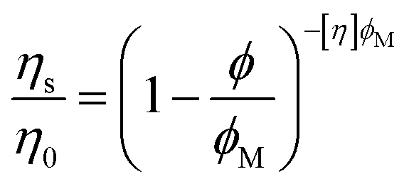 | (2) |
Polymeric dispersants are critical for controlling a complex range of phenomena in concentrated suspensions, including development of yield stress, thixotropy, jamming, and viscosity discontinuities.6 Dispersants influence all interactions in suspensions, and the physics of their effects has been studied extensively and summarized clearly.7 However, while it is possible to use these models to explain the effects of dispersants on suspensions, the inverse problem of using knowledge of these forces to design dispersants for specific suspension systems has proved exceedingly difficult. While studies on model systems have pointed to the importance of both viscous8 and osmotic forces9 in suspensions, the design principles for dispersants in complex engineering systems focus on tuning particle–particle interactions through electrostatic and steric interactions due to adsorbed polymer.10,11 Indeed, the leading dispersant for cement paste (polycarboxylate ether or PCE) is a copolymer whose function is modeled as a combination of adsorption onto charged mineral surfaces mediated by anionic monomers and steric interactions between particles mediated by pendant poly(ethylene glycol) (PEG) grafts.12–14
Machine learning is revolutionizing computational analysis and design of materials.15,16 These approaches are based on statistical analysis of datasets generated through computation17 or high-throughput experiments.18,19 The machine learning tasks in materials informatics generally center on clustering of similar materials systems or on prediction of properties, with the end goal of more efficiently searching for structures with optimal or desirable properties.20–22 This search often proceeds through large-scale screening of many candidate compounds rather than direct solution of the inverse chemical or materials design problem.23 A diversity of methods have been employed in both condensed matter and polymeric materials informatics, including random forest (e.g. ensembles of decision trees) regression models based on custom features designed through chemical intuition,24 kernel ridge regression on chemical fingerprint features,25 Gaussian process regression,26,27 dynamic Bayesian optimization of empirical models,28 and numerous other methods that can be applied to data-rich materials research.29
Regardless of which machine learning methods are applied, two fundamental challenges to progress in materials informatics are the design of the underlying numerical representations for materials systems, and incorporating the large body of domain knowledge into the structure of the machine learning models. The relationship between machine learning and condensed-matter theory is complex30 – often additional statistical analysis is used to identify descriptors with physical significance in order to gain insight into the underlying physics.31 Recent approaches in soft matter have explored using machine learning to extend theories designed for simple liquids to complex colloidal systems32 or enhancing information content from particle-tracking experiments.33 However, these methods have been developed for large computational or experimental datasets, and there is clearly a need for new approaches that are developed to provide deeper physical insight as well as prediction of material properties based on limited experimental data.
Here, a machine-learning framework for investigating suspensions is presented using sparse datasets based on simple experiments that probe the underlying forces that combine to determine changes in slurry rheology due to dispersants. Given that most published work on dispersants compares 3–5 distinct polymers,34–36 methods that facilitate statistical learning with smaller datasets make this a relevant test system. The goal was to simultaneously optimize materials structure and gain insight complex systems that are not readily modeled with strictly physical methods. The focus is on concentrated aqueous suspensions of MgO, an important material for refractory ceramics that has been also used extensively as a non-setting model for the rheology of hydraulic cement.12,37 Rather than directly attempt to correlate the chemistry of large libraries of different dispersants on concentrated-suspension properties, an intermediate tier of “single-physics” interactions (probed experimentally) is used to connect polymer composition variables with changes in rheology. This is depicted in Fig. 1. Through parametrization using basic physical models and regression analysis of these experiments, it is shown that this approach can yield insight into the effects of dispersants on particle forces, solution forces, and solution–particle interactions as well as make predictions of novel dispersants that can reduce slurry yield stress and viscosity. Discussions of uncertainty, causality, and pathways for improving and extending this approach are also presented.
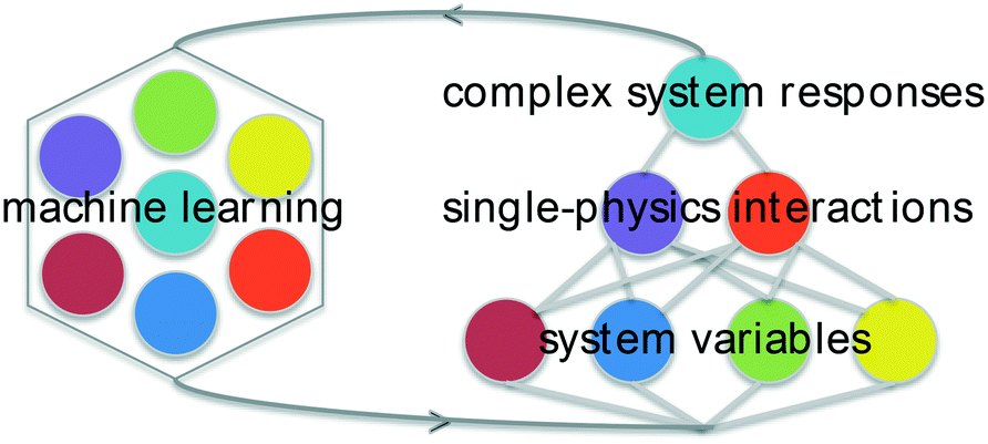 | ||
| Fig. 1 Schematic representation of hierarchical machine learning method. System variables represent a large parameter space that determine the complex system responses. Here, system variables were the functional groups and molecular architecture of the dispersants and the system responses are the yield stress and post-yield viscosity of the MgO slurry, but these are bridged using single-physics interactions that can be embedded in an intermediate tier. These interactions, which can be gauged via simple experiments, are understood to determine the system responses – in this study, the slurry rheology was assumed to depend on the solution viscosity and osmolality as well as the particle charge and electrosteric interactions that were gauged through sedimentation measurements, but no specific form was assumed a priori. Instead, statistical learning was used to uncover the structure of how the interactions determine system responses. Between the bottom and middle tiers, the system variables were connected to the single-physics interactions via simple generating equations in which viscosity, osmolality, particle charge, and particle electrosterics were parametrized by the composition variables. Integration of the models yields the system responses (yield stress and post-yield viscosity) as a function of the system variables (dispersant functional groups and architecture), which were be minimized to identify novel dispersants with high performance. | ||
Experimental
Materials
Polycarboxylate ether (PCE; Adva 190 from Grace Construction Chemicals), naphthalene sulfonate (PNS; Sika), sodium lignosulfonate (LS; Borregaard), and kraft lignin (KL; Domtar) were dialyzed for 48 hours prior to use. Polyethylene glycol (PEG, Mw: 10![[thin space (1/6-em)]](https://www.rsc.org/images/entities/char_2009.gif) 000 g mol−1) was received from Sigma and used as received. PEGylated KL (KLPEG) and LS (LSPEG) were synthesized by coupling a mesylated PEG (Mn: 750 g mol−1) in a basic aqueous solution (pH 11) to the kraft lignin and lignosulfonate following a previously reported procedure.38 Polystyrene sulfonate (PSS) was synthesized in an aqueous solution of 2 g of 4-styrenesulfonic acid sodium salt hydrate (NaSS) and 0.5 g of sodium persulfate at 80 °C for 12 h. The copolymer of polyethylene glycol methacrylate and polystyrene sulfonate (PSS-PEGMA) was synthesized by heating an aqueous solution of ethylene glycol dimethacrylate and 4-styrenesulfonic acid sodium salt hydrate in a 1:10 molar ratio at 80 °C for 12 h. For preparation of LSPC, Br-terminated PC was synthesized by ATRP of t-butyl methacrylate using ethyl α-bromoisobutyrate, pentamethyldiethylenetriamine, and copper(I) bromide (Sigma). Following deprotection, grafting onto LS was performed following the same procedure as for LSPEG. All synthesized polymers were also dialyzed for 48 hours prior to use.
000 g mol−1) was received from Sigma and used as received. PEGylated KL (KLPEG) and LS (LSPEG) were synthesized by coupling a mesylated PEG (Mn: 750 g mol−1) in a basic aqueous solution (pH 11) to the kraft lignin and lignosulfonate following a previously reported procedure.38 Polystyrene sulfonate (PSS) was synthesized in an aqueous solution of 2 g of 4-styrenesulfonic acid sodium salt hydrate (NaSS) and 0.5 g of sodium persulfate at 80 °C for 12 h. The copolymer of polyethylene glycol methacrylate and polystyrene sulfonate (PSS-PEGMA) was synthesized by heating an aqueous solution of ethylene glycol dimethacrylate and 4-styrenesulfonic acid sodium salt hydrate in a 1:10 molar ratio at 80 °C for 12 h. For preparation of LSPC, Br-terminated PC was synthesized by ATRP of t-butyl methacrylate using ethyl α-bromoisobutyrate, pentamethyldiethylenetriamine, and copper(I) bromide (Sigma). Following deprotection, grafting onto LS was performed following the same procedure as for LSPEG. All synthesized polymers were also dialyzed for 48 hours prior to use.
Concentrated aqueous suspensions containing 70% MgO (by mass) were prepared in distilled water. Suspensions were made by first dissolving the polymer in water, followed by gradually adding the MgO with ongoing stirring and shaking to evenly disperse the particles. For suspension rheology experiments, sonication was applied for a 1 h after the completion of suspension fabrication and 1 h before testing with constant stirring overnight in-between sonication. During the process, the MgO particles shed hydroxide, forming particles with zeta potentials of +20 mV in a fluid with pH of 10, an ionic strength of 2 mM, and estimated screening length of 6.8 nm.
Measurements
Adsorption of all the polymers was measured onto MgO by analyzing the total amount of carbon left in the sample before and after adsorption. Each polymer was tested at two different concentrations 0.5 and 1.0 and mixed with 5.0 wt% and 10 wt% MgO for an hour and then centrifuged to obtain the supernatant. The supernatant was subsequently diluted and the total organic carbon was measured using a GE InnovOX TOC analyzer. Zeta potential of 10 wt% MgO solutions for both 0.5 and 1.0 wt% added polymer was measured after the solutions were stirred for an hour using a Zeta-sizer (Malvern Instruments). Osmolality of aqueous solutions of all ten polymers was measured three times each for 0.1, 0.2 and 0.4 g mL−1 using a vapor pressure osmometer (Wescor 5520). The slope of the osmolality values versus concentration of all the polymer solutions was calculated and multiplied by the molar volume and molality of water to obtain the A2 coefficient. Viscosity of both the aqueous solution of the polymer with and without MgO was measured. The viscosity of both solutions was measured as a function of shear rate after 30 s of pre-shearing at 100 s−1 to erase the mixing history. The viscosity at 5 s−1 was in the linear regime for all samples and used as the representative value. These were normalized against pure water and control MgO sample respectively. The MgO pastes were tested at 70% solid content with 0.50 and 1.0 wt% polymer concentrations. Sedimentation was measured for all the polymers at three different concentrations 0.05, 0.5 and 1.0 wt% for 25 wt% loading of MgO in an aqueous solution. The height of the supernatant was measured ever 24 hours for a week. The percentage of sedimentation was calculated using the difference between the measured supernatant values at 24 h and 120 h.Computational methods
Each of the 10 polymers was represented as an equation of 8 composition variables – the first 6 were the functional groups (constrained to sum to unity) and the last two were separate architecture variables (here these could also be expressed as a single variable, but more complex architectures could be represented with multiple architecture descriptors). This formed a 10 × 8 matrix of coefficients for 8 composition variables and 10 × 5 matrix of specific polymer interaction parameter values for the set of interactions ([ηpol(![[x with combining right harpoon above (vector)]](https://www.rsc.org/images/entities/i_char_0078_20d1.gif) )], [A2()], [ζpol()], [espol()], θ()). As an overdetermined system, the least squares approximation method was employed using ‘lsqr’ function in MATLAB to get an 8 × 5 matrix of composition variables vs. specific polymer interaction parameters. The changes in the slurry viscosity at yield and post-yield viscosity due to the dispersants were expressed as functions of the estimated values of the single-physics contributions of the polymers to the following slurry parameters and responses:
)], [A2()], [ζpol()], [espol()], θ()). As an overdetermined system, the least squares approximation method was employed using ‘lsqr’ function in MATLAB to get an 8 × 5 matrix of composition variables vs. specific polymer interaction parameters. The changes in the slurry viscosity at yield and post-yield viscosity due to the dispersants were expressed as functions of the estimated values of the single-physics contributions of the polymers to the following slurry parameters and responses:
| Variable | Definition |
| η pol | Viscosity of pore solution with dissolved polymer |
| π pol | Osmotic pressure of pore solution with dissolved polymer |
| ζ pol | Zeta potential of MgO particle with adsorbed polymer |
| s pol | Sedimentation coefficient of MgO particle with adsorbed polymer |
| Δτy | Change in slurry yield stress due to polymer dispersant |
| Δηs | Change in slurry viscosity due to polymer dispersant |
The slurry parameters (ηpol, πpol, ζpol, spol) represent the single-physics interactions that underlie the slurry responses (Δτy, Δηs). In this method, the slurry responses were expressed via multiple regression using the 14 linear, quadratic, and first cross-terms of the slurry parameters. This represents the simplest approach to expressing dependence on these underlying physical variables, their magnitudes, and their couplings. Lasso and k-fold cross-validation using the cvfit function in R were used to identify a minimal set for both Δτy and Δηs. The system variables (dispersant composition and architecture) and the system responses (slurry yield stress and post yield viscosity) were connected through re-parametrizing the functions for the changes in slurry viscosity at yield and post-yield viscosity as functions of the composition variables. Here, the function for τy = τMgO + Δτy was then optimized using the fmincon solver in MATLAB, utilizing the interior point algorithm.
Results and discussion
Dispersant and concentrated suspension characterization
A library of 10 aqueous dispersants was used as a training set, and the names, abbreviations, and structures of which are shown in Fig. 2a. Except for PEO, all polymers adopt a negative charge at pH 10. The viscosity of MgO slurries was measured as a function of shear rate for each member of the training set (including the dispersant-free MgO slurry), and representative responses are shown in Fig. 2b. The peak in viscosity, which is associated with a yield stress, was 360 Pa s for the neat suspension. The shear rate at which this peak was observed had only small variation with the dispersant added, but the magnitude decreased for most of the polymers in the training set. As representative examples, incorporation of 1% LS and LSPEG both resulted in significant reductions of the yield stress, with the PEGylated analogue of LS imparting greater reductions in yield stress. In addition to the magnitude of the yield stress, the viscosity at 5 s−1 was used as a metric for the post-yield rheology. This shear rate was chosen as providing a representative measure of the post-yield rheology of the suspensions.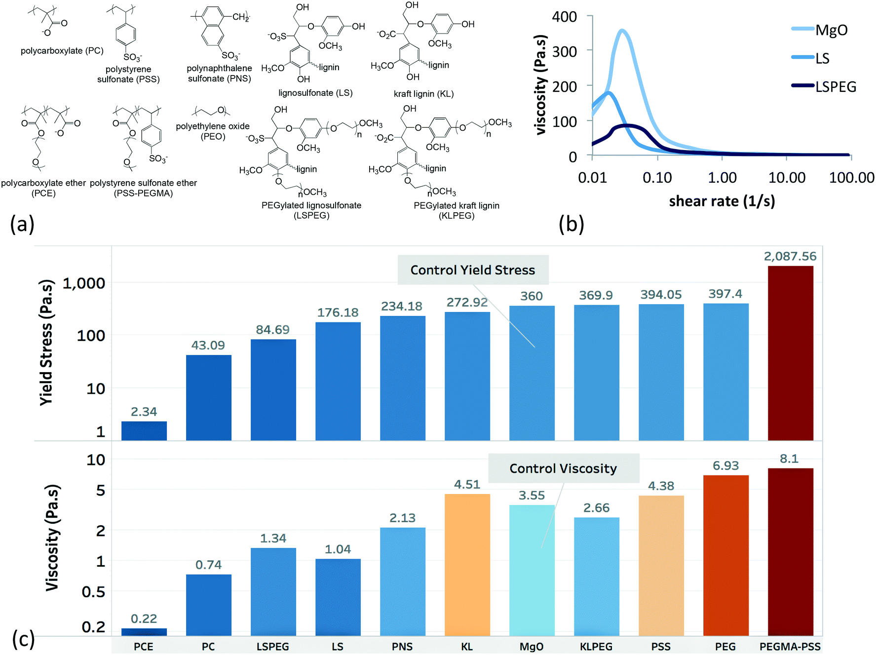 | ||
| Fig. 2 Training set used in this study. (a) Polymeric dispersants that incorporated the functional groups used as system variables. Except for PEO, all polymers adopt a negative zeta potential (summarized in ESI†) at pH 10. (b) Representative rheology data showing the viscosity as a function of steady-shear rate for the dispersant-free MgO suspension and the MgO suspension containing 1% LS. The peak in the viscosity is associated with a yielding phenomenon37 and will be referred to as the yield stress despite having units of viscosity. (c) Summary of the yield stress and post-yield viscosities for the suspensions containing 1% dispersant (note the log scales with different ranges). Many dispersants decreased both metrics, but some resulted in increases. The lowest values were recorded for the commercial PCE. For the purposes of modeling, all yield stress and viscosity values were normalized to the highest value in the training set – those of PEGMA-PSS. | ||
As a model for hydraulic cement, dispersants for MgO suspensions have anionic carboxylate or sulfonate groups to promote aqueous solubility, enhance adsorption onto charged oxide particles, and increase interparticle repulsion through electrostatic interactions. Pendant PEG groups can increase steric interactions between particles, which are known to be a much more effective dispersing mechanism than purely electrostatic forces, particularly in media with high ionic strength. Indeed, copolymers having both carboxylate and PEG functional groups are the basis for the leading commercial superplasticizer of cement (polycarboxylate ether or PCE),12–14 and the grafting of PEG onto LS has been shown to significantly reduce the yield stress of cement paste, which was attributed to an increase in steric interactions.38 Nonpolar alkyl and aromatic groups on these polymers act as a framework for presentation of polar groups but can also function to determine the balance of free vs. adsorbed dispersant in the suspension.
It should be noted that all the crosslinked members of the training set are lignin-based. Lignins, and lignosulfonates in particular, are an important class of dispersant that finds broad use in industrial formulations.39 However, many lignins are thought to have a sheet-like architecture40 whereas an approximately spherical architecture is common for discrete synthetic polymers with crosslinked architecture, such as star copolymers.41 Thus, the model understands the crosslinked variable to represent a sheet-like architecture, and synthesis of these predictions will involve chemical modification of lignin.
Finally, it is thought that yielding is determined by dissociation or fracture of a percolating particle network while the post-yield viscosity is thought to be dominated by the dynamic aggregation number of flocs in suspension under shear flow.42 The challenge is in predicting how the functional-group composition and architecture of the dispersants simultaneously tune particle, solution, and particle–solution interactions in determining these rheological responses.
Parametrization of single-physics experiments by polymer composition
The first step in the model was to connect the bottom tier (polymer composition) with the middle tier (single-physics interactions), which was accomplished by parametrizing the basis set of interactions that determined slurry rheology in terms of polymer composition. A set of continuous composition variables that describe the distribution of functional groups in the polymers, along with one discrete variable indicating polymer architecture (crosslinked vs. linear) were used as a simple representation. The goal was to develop simple, physically informed models for predicting changes in solution viscosity, solution osmolality, particle sedimentation, and particle zeta potential in the actual concentrated suspension as functions of the composition of the dispersant. Each of these models were parameterized to fit measurements in commonly performed experiments.The composition of each polymer was expressed as mole fractions of functional groups assuming a constant molecular weight for each dispersant of 17 kDa, which is the mean for this training set. The groups considered here were aromatic, alkyl, linear PEO, sulfonate, carboxylate, and pendant PEG grafts. The functional groups were defined on the basis of synthetic accessibility rather than on the basis of molecular volume. For example, alkyl groups included ca. 3 CHx moieties, aromatic groups were based on C6H6 fragments, and PEG grafts were composed of 8 (CH2OCH2) monomers. Architecture was approximated as either crosslinked or linear. Thus each dispersant is represented by an eight-element feature vector of these composition variables, which are summarized in ESI.†
The single-physics interactions represented the forces that were thought to underlie the complex responses of the slurry to the dispersants. Two solution forces (viscosity and osmolality) and two particle forces (electrostatic and electrosteric) formed a basis set for expressing the responses, and they were measured individually in simple experiments that directly probed the solution variables or indirectly probed the particle variables. For the latter, zeta potential was taken as a measure of particle charge, and particle sedimentation in dilute suspensions was used to gauge electrosteric forces. The goal was to extract specific contributions of each functional group to the single-physics interactions by estimating the polymer contribution to each of these interactions in the suspensions (ηpol, πpol, ζpol, spol). This was accomplished by parametrizing the basis set in terms of the functional groups by fitting data for each at multiple concentrations and measuring the partition coefficient θ. This results in a prediction of the basis set parameters as a function of composition, which are summarized in ESI.†
These composition features and the single-physics interactions are illustrated schematically in Fig. 3. The subscript “pol” for each of the single-physics variables reinforces that the model is designed to reflect changes due to the presence of the polymer. Square brackets “[…]” denote a specific parameter that is scaled to polymer concentration in solution or coverage of adsorbed polymer on the particle surface.
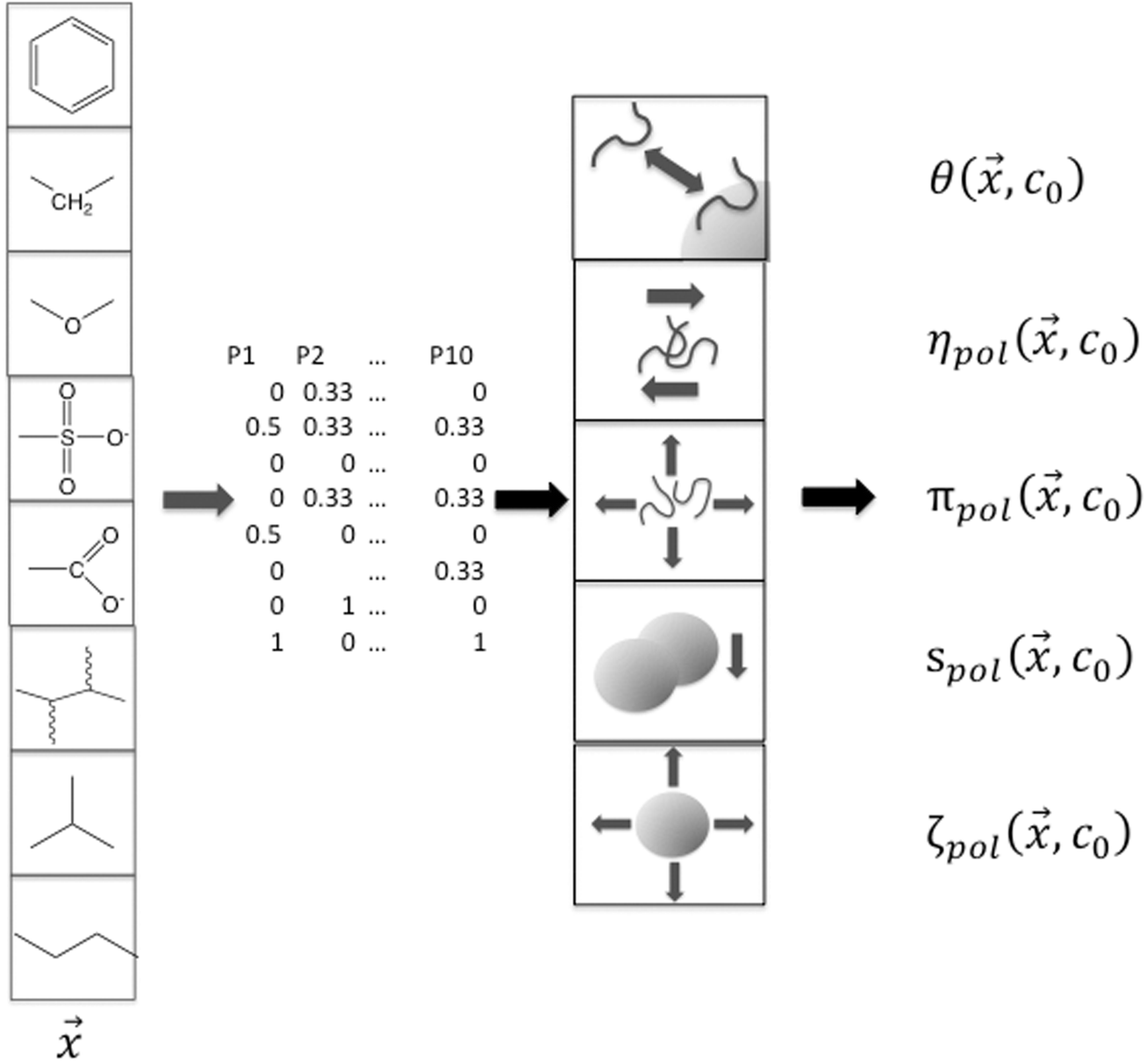 | ||
| Fig. 3 Schematic representation of connecting the dispersant composition and architecture variables with single-physics interactions based on experimental measurements. | ||
While not used directly as a variable for expressing yield stress or slurry viscosity, the coverage of polymer on particle surfaces is a measure of the partitioning between free and adsorbed states, which is critical for understanding dispersant effects on the solution properties against effects on the particle characteristics. It should be noted that the maximum estimated MgO coverage in the training set was 65% for PSS, which is well below saturation limit of adsorption. Transitions from thixotropic to Newtonian behavior with concomitant reductions in viscosity have been reported in the effective coverage range of 68–96%, which were well fit by the Casson equation.43 In the present work, however, the data and resulting model are limited to below saturation.
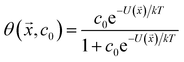 | (3) |
The interaction potential U was assumed to be that for a single polymer rather than for a monomer, which is the rigorous approach to polymer adsorption,44 and this was further parametrized by the fraction of each functional group in using least squares estimation. This generated a map from polymer composition to adsorption energy and then to coverage, albeit an approximate one given the small sample size.
The solution viscosity was parametrized by polymer concentration by assuming the viscosity to vary linearly with concentration of dissolved polymer c0(1 − θ). The specific viscosity reflects differences in contribution due to each polymer, which is always positive relative to the viscosity of pure water and takes the form:
| ηpol = c0(1 − θ)[ηpol()] | (4) |
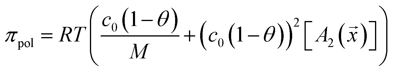
The virial coefficient A2 was measured for each polymer and used to estimate the solution osmolality assuming the molecular weight for each polymer had a constant value of 17 kDa. This can be positive or negative depending on the solubility of the polymer in water at pH 10 but the net osmotic pressure is always positive.
 | (5) |
The zeta potential ζ for each polymer was measured in solution having pH 10. The zeta potential for the bare MgO particles in solution was found to be +20 mV, and the differential effect on the zeta potential of MgO particles with adsorbed polymer were assumed to take the form:
| ζpol = c0θ[ζpol()] | (6) |
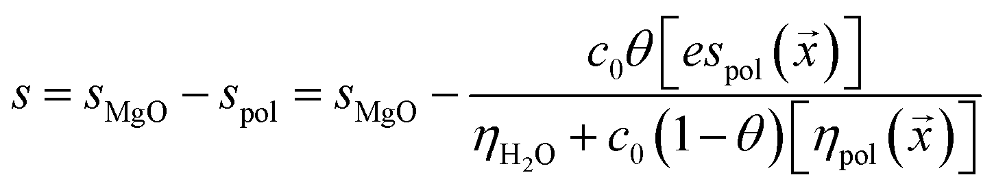
Electrosteric interactions between particles with adsorbed polymer are exceedingly complex to measure and model.11 Here, the sedimentation parameter s, defined as the ratio of the particle velocity and the acceleration (s = v/a), was used as a gauge of these interactions. The Stokes equation predicts that it varies as d2/ηsol where d is the particle diameter and ηsol is the solution viscosity. In this approach, s is assumed to be reduced relative to that of a neat MgO solution (denoted by sMgO) due to a combination of a specific electrosteric interaction parameter espol multiplied by the estimated coverage c0θ() divided by the estimated solution viscosity. The change in the sedimentation coefficient due to the adsorbed polymer can be positive or negative, depending on how these polymers influence particle–particle interactions.
 | (7) |
The results of decomposing the specific polymer interaction parameters ([ηpol()], [A2()], [ζpol()], [espol()]) across the composition array yielded the functional-group contributions to each interaction. The concentration dependence is captured in changes in the coverage θ; all other interaction parameters were assumed to be concentration-independent.
While θ was not explicitly included as a single-physics interaction, it plays a critical role in determining the balance of solution-based vs. particle-based effects. Indeed, this appears to be the basis for some of the positive and negative correlations between the specific polymer interaction parameters. However, it should be noted here that explicitly including both solution-based and particle-based contributions in the models for the slurry rheology balances the partitioning between these phases.
Regression analysis of slurry yield stress and viscosity
In this method, the complex system responses yield stress and slurry viscosity were assumed to be functions of the single-physics interactions. Models for the changes in yield stress and viscosity (both usually negative) due to the addition of polymer were fit via regularized polynomial regression on the single-physics interactions. While it is possible to use more complex, empirical equations that have been shown to fit experimental data well (e.g. viscoelastic responses45), in this preliminary work only functions based on the 14 first- and second-order terms (including the first cross-terms) of (ηpol, πpol, ζpol, spol) were considered. However, a statistical method is needed to identify the minimal set of these variables that both accurately model the training set but also provide the broadest generalization to predicting the behavior of new dispersants.The standard linear regression model can be formulated as minw(∥Xw − y∥22) where X is a given input matrix, y denotes output vector (system responses Δτy or Δηs), and w is the vector of model parameters to be optimized (taken from (ηpol, πpol, ζpol, spol)). The challenge was to identify the minimal essential parameters in the model that provide both the best fit to the training data but also the greatest predictive accuracy. The Lasso algorithm46 extends the standard linear regression to:
| minw(∥Xw − y∥22 + λ∥w∥1) | (8) |
We applied Lasso to obtain separate models of the slurry yield stress and viscosity in terms of the single-physics interactions. For each case, we used the grid search approach with leave-one-out cross-validation (LOOCV) to select the regularization parameter in the range 0.001 ≤ λ ≤ 5. The grid search validation results for both the slurry yield stress and viscosity are plotted in Fig. 4. Each of these corresponded to the optimal balance of increasing regularization, in terms of both reduction of model prediction error and model variance.
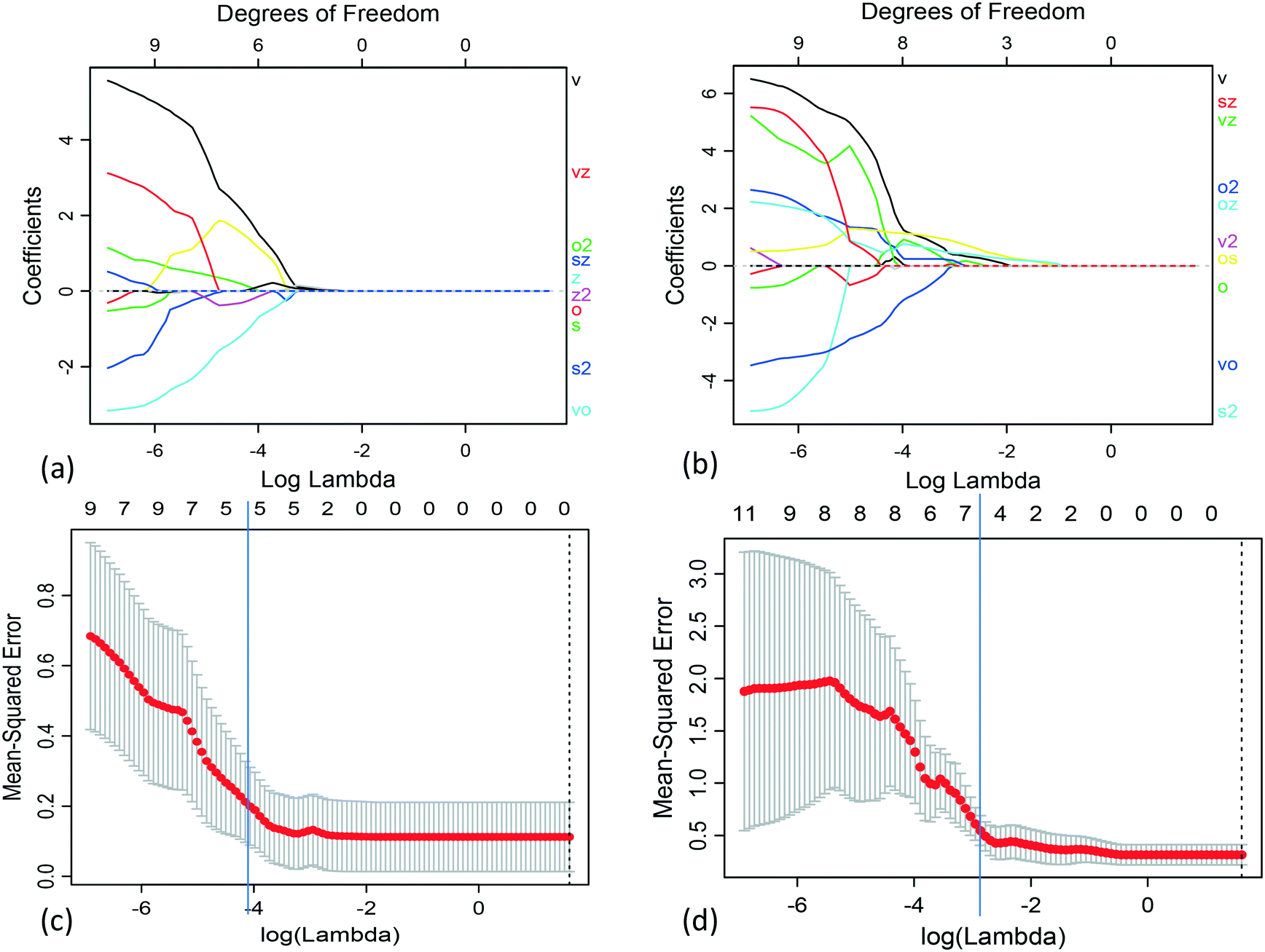 | ||
| Fig. 4 Lasso path for determining the minimal variables with best fit to represent the slurry yield stress (left) and viscosity (right) as a function of polynomials in (ηpol, πpol, ζpol, spol). Starting with the full basis set of 14 variables, Lasso increasingly suppressed regression coefficients as λ was increased, which is shown in (a) and (b). In (c) and (d) are shown the validation mean squared prediction error (MSE) for both the yield stress and viscosity models. As indicated in (c) and (d), we selected regularization parameters λ = 0.02 for the yield stress model and λ = 0.03 for the viscosity model. | ||
After independent selection of regularization parameters for the viscosity and yield stress models through LOOCV, Lasso performed on the entire training set resulted in the following final models for Δτy and Δηs:
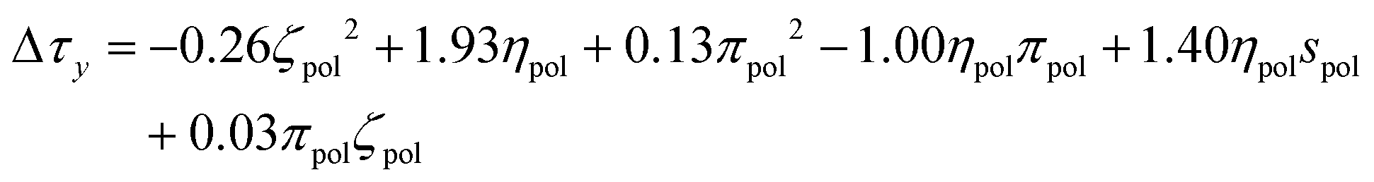 | (9) |
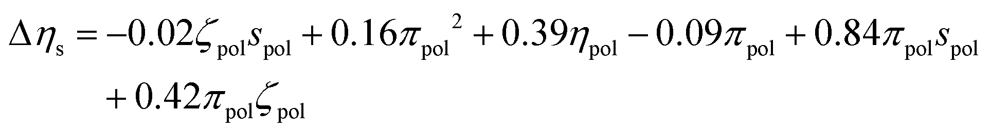 | (10) |
Each term in these expressions relates to the differential effects of given variables on slurry properties relative to the unmodified slurry yield stress τMgO and viscosity ηMgO, respectively. In the current form of the changes in yield stress and slurry viscosity, the coefficients have units necessary to convert the normalized polynomial terms to the corresponding units. The values of the solution variables ηpol and πpol were normalized to [0,1] but the particle variables ζpol and spol were normalized to [−1,1] to allow for the full range of particle characteristics. Thus, the relative contributions of each term could increase or decrease the overall yield stress or post-yield viscosity depending on the sign of the coefficient and the sign and functional form of the variable. For example, the yield stress was reduced by changes in particle zeta potential as −0.26ζpol2 (physically reasonable being independent of sign of the potential) while post-yield viscosity was predicted to increase with changes in solution viscosity as 0.39ηpol. In contrast, a number of terms represented coupling between particle and solution variables, and their relative contributions to changes in the rheological properties depended on both the signs of the coefficients as well as the signs of the variables themselves.
It is difficult to determine standard errors from penalized regression methods such as the Lasso.47 Sandwich formulas have been explored but only provide variance estimates for non-zero coefficients,48,49 while other approaches involving covariance matrices can have complex distributions that are not readily interpreted.50,51 Given these challenges, the question of uncertainty in the exact numerical form of the model will be deferred, and its physical significance and predictions will instead be explored.
The polynomials in eqn (9) and (10) represent a statistical approach to determining the effects of changes in particle and solution characteristics on slurry rheology. However, for the purposes of gaining physical insight into their significance, the terms in both equations can be divided into three groups: particle properties due to zeta potential or sedimentation interactions, solution properties due to viscosity or osmolality, and coupling between particle and fluids variables. The contributions of these individual effects can be captured in plots of four representative polymers to illustrate the effects of particular functional groups or architectures. This is shown in Fig. 5 for PCE, LSPEG, LS, and PNS for contributions to both the yield stress and viscosity.
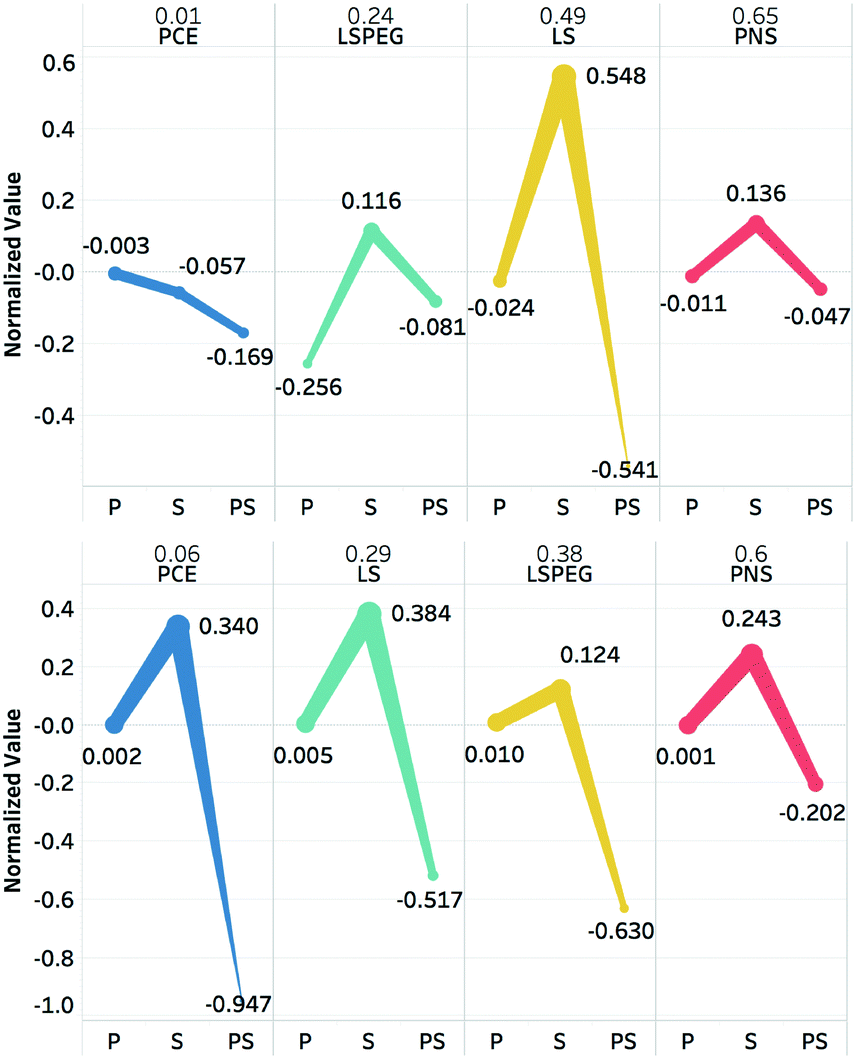 | ||
| Fig. 5 Plots of changes in slurry yield stress (top) and viscosity (bottom) due to PCE, LS, LSPEG, or PNS described by particle (P), solution (S), and solution–particle (PS) interaction variables. The corresponding polymer is labeled at the top of each panel along with the resulting yield stress or viscosity expressed as a fraction of the corresponding value relative to the dispersant-free MgO suspension. The commercial PCE resulted in the smallest values for both yield stress and viscosity. | ||
The value of the slurry yield stress or viscosity due to a given polymer (relative to the value for slurry without dispersant) is represented as a fraction above the dispersant abbreviation, and the normalized contributions of the respective particle (P), solution (S), and particle–solution (PS) terms to this value are plotted for each polymer as separate categories. For example, to calculate the solution contribution to the yield stress for a given polymer, the calculated values of ηpol and πpol, which were then used to calculate 1.93ηpol + 0.13πpol2 − 1.00ηpolπpol. Note that the regression model actually predicted a slight increase in yield stress (Δτy > 0) for PNS, in contrast, the measured decrease and is why the sum of the parameters is positive. However, for the other dispersants in the training set, especially those where that impart greater changes in slurry rheology, there was generally good agreement between predicted and measured values.
For the yield stress, it is seen that all three terms for PCE contribute to reductions in this metric, but for the other polymers the solution terms all contribute increases, which must be offset by the particle and particle–solution contributions. It is also interesting to compare the effects of PEGylation on the effects of LS to the yield stress. Whereas LS had minimal effects on the particle contribution while it had a large, positive contribution to solution variables and a large negative contribution to particle–solution variables, which nearly offset each other. For LSPEG, the solution contribution was less positive and the particle contribution was significantly more negative, which may be attributed to the solubilizing effects and steric interactions imparted by the PEG grafts.
In tuning the post-yield viscosity, all four dispersants had particle contributions near zero and positive solution contributions, with LSPEG having the lowest value. However, these were offset for PCE, LS, and LSPEG by strongly negative particle–solution terms. This is consistent with the predictions of theoretical modeling that suggested coupling between adsorbed and free polymer via osmotic forces, which can strongly stabilize suspensions.52
While the preliminary approach outlined here relies on a number of simplifications to create a tractable methodology, the end results appear to largely align with basic intuition for these complex systems but offers clarity in terms of decomposing the effects into physically meaningful contributions. Thus, the methodology naturally provides physical insight. However, the meaningful test comes in validating its predictions for dispersants that minimize metrics of slurry rheology.
Hierarchical integration and optimization
Integration of the tiers in the model results in re-parametrization of the expressions for changes in slurry yield stress and viscosity in terms of polymer composition and concentration: Δτy = Δτy(,c0) and Δηs = Δηs(,c0). The model was first evaluated by comparing the predictions of the yield stress from the model to those from a simple direct statistical comparison using the 10 polymers in the training set.
Minimization of these functions with respect to composition and concentration provided specific targets for the molecular engineering of dispersants in this suspension system. It should be noted that while strictly statistical approaches based on library screening can only identify synergies through directly probing those specific regions of the parameter space, inclusion of the physical relationships in the middle tier of the methodology can, in principle, anticipate synergistic effects that can lead to local or global extrema in responses as a function of composition.
The Fmincon (interior point algorithm) optimization routine in MATLAB was used to identify minima in yield stress as a function of composition. Interestingly, unconstrained optimization resulted in a negative divergence of the function Δτy(,c0) and provided compositions that had only one or two functional groups – pure PEG grafts in a linear polymer architecture or a crosslinked polymer with 75% carboxylate and 25% aromatic content. However, a constrained optimization requiring the total yield stress to be positive (τMgO + Δτy ≥ 0) and the concentration to be less than 2% resulted in a predicted a composition that contained all the functional groups in specific ratios, listed in Fig. 6, at a concentration of 0.75%. Uncertainty in the predicted yield stress values was based on function tolerances rather than standard errors, and convergence was assumed at 1 × 10⁻⁶.
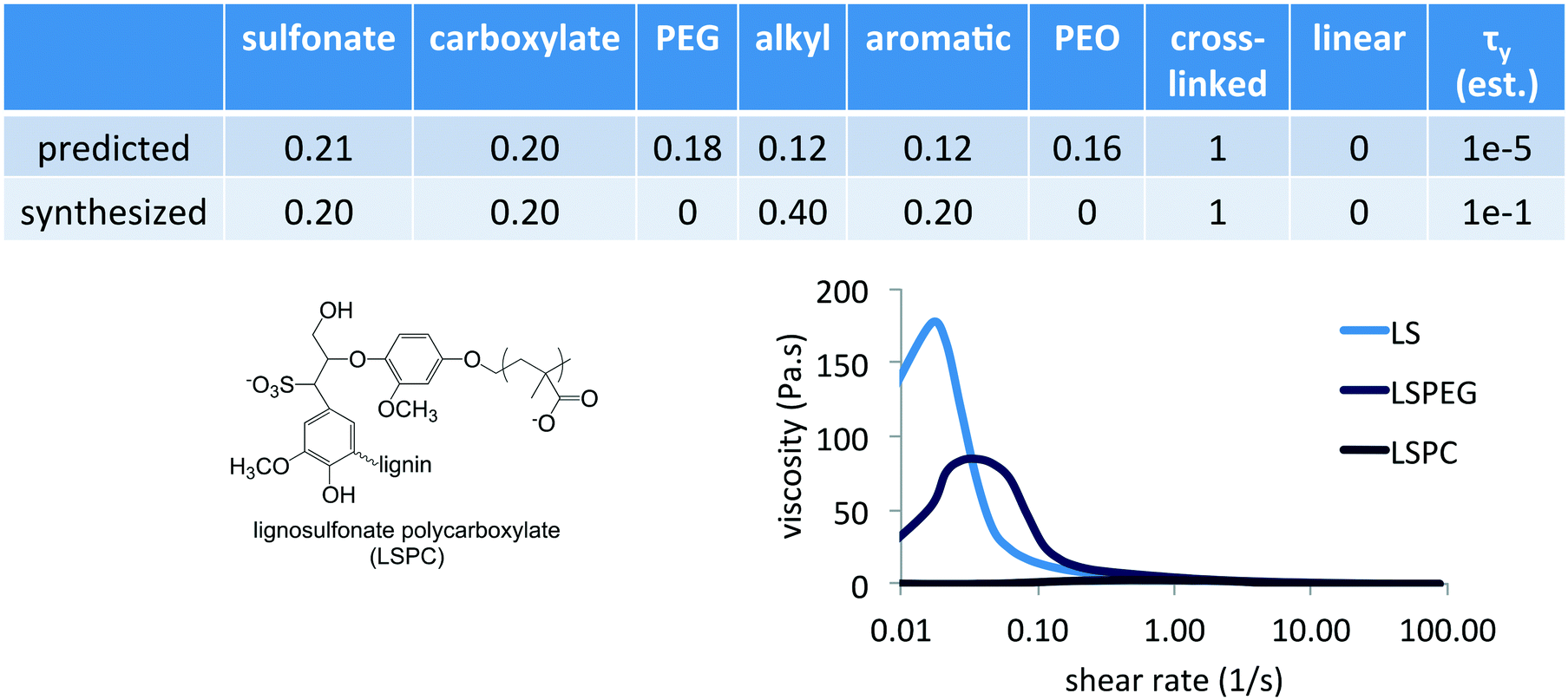 | ||
| Fig. 6 Prediction of the dispersant composition that minimizes the overall yield stress under constrained optimization (τMgO + Δτy ≥ 0) and the composition of polycarboxylate-grafted lignosulfonate (LSPC) that was synthesized to test it. The estimates of the slurry viscosity at yield from the model are included in the final column as a fraction of the viscosity at yield of the neat MgO slurry (360 Pa s). The schematic representation of LSPC is shown to the left, and the rheology traces comparing MgO suspensions with 1% LS, LSPEG, and LSPC are shown at the right. On this scale, the LSPC curve is visible just above the baseline. | ||
One drawback of the simple representation of polymer composition and architecture that was used in this preliminary study is that synthesizing predictions of the model requires interpretation and selection from numerous alternatives. In terms of the composition variables, which are ultimately the independent variables, it was clear from the predicted composition that an important feature was the combination of sulfonate and carboxylate groups in a crosslinked architecture having alkyl and aromatic groups. In synthesizing a similar composition, no PEG grafts or long PEO chains were included to allow the identification of specific contributions of this combination of charged groups. Given that PEGylation of LS imparted a lower yield stress, an alternative modification strategy for LS was explored to incorporate carboxylate groups in which a smaller PC was used instead as the graft to impart both this functionality as well as possible steric interactions. PC was synthesized via atom transfer radical polymerization and grafted onto LS in pH 10 solution via the reactive Br-terminus following similar conditions as previously reported. This resulted in a grafted architecture similar to LSPEG but with an anionic PC corona having average DP of 26 and a grafting density of 2 PC per LS, similar to the size and grafting density of PEGylation in LSPEG. The synthesized composition is listed in Fig. 6 to compare with that predicted.
The PC-grafted LS imparted a yield stress in MgO suspensions that was nearly identical to that of the commercial PCE (<5 Pa s), despite being based on a crosslinked, aromatic architecture instead of a linear anionic polymer with pendant PEG grafts. This high level of performance made a subsequent learning step, in which the results of the predicted composition were included in the training set and the model was refined, unnecessary for the immediate goal of demonstrating the method. However, the modeling clearly points to an unexpectedly rich region of the variable space and probing structure–function relationships will yield further insights into dispersant design. While the representation of polymer composition in terms of mole fraction ultimately requires judicious interpretation of the model predictions, even this simple approach to hierarchical machine learning can identify critical components necessary to incorporate into next-generation dispersants. More sophisticated representations of molecular functionality and architecture would require a larger training set, but this method requires far fewer samples in training sets whose sizes are approximately linear in the number of parameters as opposed to strictly statistical approaches that require far denser coverage of variable spaces.
A final issue that needs to be addressed is that of causality.53,54 In seeking to optimize performance, correlations between system variables and responses could be satisfactory, but gaining deeper insight into complex physical phenomena from this approach requires establishing causal relationships. In this hierarchical approach, causality needs to be established between the system variables and the single-physics interactions as well as the determining whether the single-physics interactions used as a basis set here accurately represent the physics of dispersant function in suspensions.
Conclusion
Adapting machine learning methods for analyzing and making predictions based on sparse datasets is critical for advancing experimental research in complex material systems. This requires strategies for integrating statistical and physical modeling, and hierarchical machine learning represents a new approach for this. In addition to allowing predictions based on limited sample sizes, the integration of physical modeling anticipates synergies between system variables that could only be uncovered in purely statistical approaches through exhaustive screening. This method could find broad application across complex physical systems that are not addressable by current computational methods but are also not amenable to high-throughput experimentation.Acknowledgements
This work was supported in part by funding from the National Science Foundation (CBET-1510600). Profs. Elizabeth Holm and Markus Deserno are gratefully acknowledged for helpful discussions. Mr. Timothy Kelly generated the Table of Contents graphic.References
- S. H. Strogatz, Nature, 2001, 410, 268–276 CrossRef CAS PubMed.
- N. Israeli and N. Goldenfeld, Phys. Rev. Lett., 2004, 92 Search PubMed.
- A. J. Liu, G. S. Grest, M. C. Marchetti, G. M. Grason, M. O. Robbins, G. H. Fredrickson, M. Rubinstein and M. O. de la Cruz, Soft Matter, 2015, 11, 2326–2332 RSC.
- G. N. Choi and I. M. Krieger, J. Colloid Interface Sci., 1986, 113, 101–113 CrossRef CAS.
- L. Struble and G. K. Sun, Adv. Cem. Based Mater., 1995, 2, 62–69 CrossRef CAS.
- J. Mewis and N. J. Wagner, Colloidal suspension rheology, Cambridge University Press, Cambridge, New York, 2012 Search PubMed.
- J. A. Lewis, J. Am. Ceram. Soc., 2000, 83, 2341–2359 CrossRef CAS.
- A. B. Metzner, J. Rheol., 1985, 29, 739–775 CrossRef CAS.
- W. C. K. Poon, J. Phys.: Condens. Matter, 2002, 14, R859–R880 CrossRef CAS.
- J. Clayton, Surf. Coat. Int., Part B, 1997, 80(9), 414–420 CrossRef CAS.
- R. J. Flatt, I. Schober, E. Raphael, C. Plassard and E. Lesniewska, Langmuir, 2009, 25, 845–855 CrossRef CAS PubMed.
- Y. F. Houst, P. Bowen, F. Perche, A. Kauppi, P. Borget, L. Galmiche, J. F. Le Meins, F. Lafuma, R. J. Flatt, I. Schober, P. F. G. Banfill, D. S. Swift, B. O. Myrvold, B. G. Petersen and K. Reknes, Cem. Concr. Res., 2008, 38, 1197–1209 CrossRef CAS.
- G. H. Kirby and J. A. Lewis, J. Am. Ceram. Soc., 2004, 87, 1643–1652 CrossRef CAS.
- K. Yamada, T. Takahashi, S. Hanehara and M. Matsuhisa, Cem. Concr. Res., 2000, 30, 197–207 CrossRef CAS.
- K. Rajan, Annu. Rev. Mater. Res., 2015, 45, 153–169 CrossRef CAS.
- A. A. White, MRS Bull., 2013, 38, 594–595 CrossRef.
- S. Curtarolo, G. L. W. Hart, M. B. Nardelli, N. Mingo, S. Sanvito and O. Levy, Nat. Mater., 2013, 12, 191–201 CrossRef CAS PubMed.
- B. L. DeCost and E. A. Holm, Comput. Mater. Sci., 2015, 110, 126–133 CrossRef.
- M. L. Green, I. Takeuchi and J. R. Hattrick-Simpers, J. Appl. Phys., 2013, 113 Search PubMed.
- A. Agrawal and A. Choudhary, APL Mater., 2016, 4, 053208 CrossRef.
- R. J. Needs and C. J. Pickard, APL Mater., 2016, 4, 053210 CrossRef.
- K. Rajan, Annu. Rev. Mater. Res., 2015, 45, 153–169 CrossRef CAS.
- R. Olivares-Amaya, C. Amador-Bedolla, J. Hachmann, S. Atahan-Evrenk, R. S. Sanchez-Carrera, L. Vogt and A. Aspuru-Guzik, Energy Environ. Sci., 2011, 4, 4849–4861 CAS.
- B. Meredig, A. Agrawal, S. Kirklin, J. E. Saal, J. W. Doak, A. Thompson, K. Zhang, A. Choudhary and C. Wolverton, Phys. Rev. B, 2014, 89, 094104 CrossRef.
- G. Pilania, C. Wang, X. Jiang, S. Rajasekaran and R. Ramprasad, Sci. Rep., 2013, 3, 2810 CrossRef PubMed.
- P. V. Balachandran, D. Xue, J. Theiler, J. Hogden and T. Lookman, Sci. Rep., 2016, 6 Search PubMed.
- D. Xue, P. V. Balachandran, J. Hogden, J. Theiler, D. Xue and T. Lookman, Nat. Commun., 2016, 7 Search PubMed.
- R. Dehghannasiri, D. Xue, P. V. Balachandran, M. R. Yousefi, L. A. Dalton, T. Lookman and E. R. Dougherty, Comput. Mater. Sci., 2017, 129, 311–322 CrossRef CAS.
- S. R. Kalidindi and M. De Graef, Annu. Rev. Mater. Res., 2015, 45, 171–193 CrossRef CAS.
- N. Wagner and J. M. Rondinelli, Front. Mater., 2016, 3, 28 Search PubMed.
- L. M. Ghiringhelli, J. Vybiral, S. V. Levchenko, C. Draxl and M. Scheffler, Phys. Rev. Lett., 2015, 114 Search PubMed.
- A. W. Long, C. L. Phillips, E. Jankowksi and A. L. Ferguson, Soft Matter, 2016, 12, 7119–7135 RSC.
- A. Yevick, M. Hannel and D. G. Grier, Opt. Express, 2014, 22, 26884–26890 CrossRef PubMed.
- S. Creutz, R. Jerome, G. M. P. Kaptijn, A. W. van der Werf and J. M. Akkerman, J. Coat. Technol., 1998, 70, 41–46 CrossRef CAS.
- D. Marchon, U. Sulser, A. Eberhardt and R. J. Flatt, Soft Matter, 2013, 9, 10719–10728 RSC.
- L. R. Murray, C. Gupta, N. R. Washburn and K. A. Erk, J. Colloid Interface Sci., 2015, 459, 107–114 CrossRef CAS PubMed.
- L. R. Murray and K. A. Erk, J. Appl. Polym. Sci., 2014, 131, 40429 CrossRef.
- C. Gupta, K. M. Perkins, R. T. Rios and N. R. Washburn, Adv. Cem. Res., 2017, 29, 2–10 CrossRef.
- M. Norgren and H. Edlund, Curr. Opin. Colloid Interface Sci., 2014, 19, 409–416 CrossRef CAS.
- P. Luner and U. Kempf, Tappi, 1970, 53, 2069 CAS.
- G. Kreutzer, C. Ternat, T. Q. Nguyen, C. J. G. Plummer, J. A. E. Manson, V. Castelletto, I. W. Hamley, F. Sun, S. S. Sheiko, A. Herrmann, L. Ouali, H. Sommer, W. Fieber, M. I. Velazco and H. A. Klok, Macromolecules, 2006, 39, 4507–4516 CrossRef CAS.
- R. A. Day, B. H. Robinson, J. H. R. Clarke and J. V. Doherty, J. Chem. Soc., Faraday Trans. 1, 1979, 75, 132–139 RSC.
- L. C. Guo, Y. Zhang, N. Uchida and K. Uematsu, J. Am. Ceram. Soc., 1998, 81, 549–556 CrossRef CAS.
- J. M. H. M. Scheutjens and G. J. Fleer, J. Phys. Chem., 1979, 83, 1619–1635 CrossRef CAS.
- N. W. Tschoegl, The phenomenological theory of linear viscoelastic behavior: an introduction, Springer-Verlag, Berlin, New York, 1989 Search PubMed.
- R. Tibshirani, J. R. Stat. Soc. Series B Stat. Methodol., 1996, 58, 267–288 Search PubMed.
- M. Kyung, J. Gill, M. Ghosh and G. Casella, Bayesian anal., 2010, 5, 369–411 CrossRef.
- J. Q. Fan and R. Z. Li, J. Am. Stat. Assoc., 2001, 96, 1348–1360 CrossRef.
- H. Zou, J. Am. Stat. Assoc., 2006, 101, 1418–1429 CrossRef CAS.
- M. R. Osborne, B. Presnell and B. A. Turlach, J. Comput. Graph. Stat., 2000, 9, 319–337 Search PubMed.
- B. M. Potscher and H. Leeb, J. Multivar. Anal., 2009, 100, 2065–2082 CrossRef.
- A. P. Gast and L. Leibler, J. Phys. Chem., 1985, 89, 3947–3949 CrossRef CAS.
- T. Claassen and T. Heskes, presented in part at Advances in Neural Information Processing Systems, Vancouver, Canada, December, 2010 Search PubMed.
- K. Zhang and A. Hyvärinen, presented in part at Proceedings of the twenty-fifth conference on uncertainty in artificial intelligence, Montreal, Canada, June, 2009 Search PubMed.
Footnote |
| † Electronic supplementary information (ESI) available. See DOI: 10.1039/c7me00027h |
| This journal is © The Royal Society of Chemistry 2017 |