
 Open Access Article
 This Open Access Article is licensed under a Creative Commons Attribution-Non Commercial 3.0 Unported Licence
Proteomics profiling of interactome dynamics by colocalisation analysis (COLA)†
Faraz K.
Mardakheh‡
*a,
Heba Z.
Sailem‡
ab,
Sandra
Kümper
a,
Christopher J.
Tape
 ac,
Ryan R.
McCully
a,
Angela
Paul
a,
Sara
Anjomani-Virmouni
a,
Claus
Jørgensen
d,
George
Poulogiannis
a,
Christopher J.
Marshall§
a and
Chris
Bakal
*a
ac,
Ryan R.
McCully
a,
Angela
Paul
a,
Sara
Anjomani-Virmouni
a,
Claus
Jørgensen
d,
George
Poulogiannis
a,
Christopher J.
Marshall§
a and
Chris
Bakal
*a
aInstitute of Cancer Research, Division of Cancer Biology, 237 Fulham Road, London SW3 6JB, UK. E-mail: chris.bakal@icr.ac.uk; mardakheh@icr.ac.uk
bInstitute of Biomedical Engineering, University of Oxford, Old Road Campus Research Building, Oxford OX3 7DQ, UK
cDepartment of Biological Engineering, Massachusetts Institute of Technology, Cambridge, Massachusetts 02139, USA
dCancer Research UK Manchester Institute, University of Manchester, Wilmslow Road, Manchester M20 4BX, UK
First published on 1st November 2016
Abstract
Localisation and protein function are intimately linked in eukaryotes, as proteins are localised to specific compartments where they come into proximity of other functionally relevant proteins. Significant co-localisation of two proteins can therefore be indicative of their functional association. We here present COLA, a proteomics based strategy coupled with a bioinformatics framework to detect protein–protein co-localisations on a global scale. COLA reveals functional interactions by matching proteins with significant similarity in their subcellular localisation signatures. The rapid nature of COLA allows mapping of interactome dynamics across different conditions or treatments with high precision.
Introduction
Systems level understanding of biological processes requires unravelling of functional interactions on a global scale. A functional interaction is a molecular association between two or more proteins which share a common, interdependent, biological function. Mining of such interactions on a global scale is often achieved by high-throughput genetic screens,1 where interactions are inferred by commonality in phenotypic outcomes of genetic gain or loss of function events.2,3 Alternatively, functional interactions can be inferred from molecular interaction analyses, on the principle of ‘guilt by association’.4 Determining such interactions on a global scale, however, has remained a fundamental technical challenge. Reporter based methods such as Yeast-2-Hybrid (Y2H) or protein-fragment complementation assay (PCA) are labour intensive, and can only reveal direct biochemical interactions.5,6 Affinity Purification coupled with Mass Spectrometry (AP-MS),7,8 or proximity based labelling,9 are similarly labour intensive, but do reveal indirect interactions. A major downside of both AP-MS and proximity based labelling methods, however, is that the analysis time is directly proportional to the number of proteins being investigated, rendering large scale comparative interactome analysis across different conditions difficult due to an increasing number of mass spectrometry runs. Moreover, tagging of cellular proteins required for both methods could affect their activity, resulting in potential artefacts.Recently, a novel proteomics based approach has been utilised to reveal interactions by assessing the co-behaviour of interacting proteins when biochemically fractionated.10 Havugimana et al. used three parallel chromatography methods in conjugation with proteomics, separating soluble cellular complexes based on charge, pKa, and density.11 Kristensen et al., on the other hand, used size-exclusion chromatography in conjugation with proteomics to separate complexes by size.12 Proteins with similar elution profiles were then matched as likely constituents of the same complexes. The key advantage of these approaches is allowing simultaneous determination of biochemical interactions from a fixed number of mass spectrometry runs.12,13 However, a downside of both approaches is that they are limited to soluble proteins, and therefore are not well suited for detecting insoluble complexes. Moreover, while matching proteins based on biochemical co-fractionation can reveal strong associations that survive such fractionations, many physiologically relevant functional interactions only occur transiently, thus are often missed during stringent biochemical separations.9
Eukaryotic cells are highly compartmentalised assembly of organelles, macro-molecular complexes, and spatially organised subcellular functional regions. As a result, where a protein is localised inside a eukaryotic cell can be indicative of its function. More importantly, colocalisation of two or more proteins can be indicative of their functional interaction.14 We hypothesised that, similar to multi-variate phenotypic signatures used in high-throughput genetic interaction analyses,2 quantitative multi-dimensional subcellular localisation signatures can be used to match functionally interacting proteins on the basis of their colocalisation. We here present COLA, a streamlined proteomics–bioinformatics strategy to infer functional interactions from significant similarities in subcellular localisation patterns. COLA uses complete subcellular fractionation in conjugation with quantitative proteomics to generate a quantitative, multi-dimensional, subcellular localisation signature for each identified cellular protein. Bootstrapped hierarchical clustering is then used to match proteins with significant similarity in their localisation signatures. Crucially, COLA is not limited to soluble protein complexes, and can reveal functional interactions on a global scale based on subcellular proximity with high Precision and Sensitivity. Finally, by utilising Tandem-Mass-Tagging for quantitative profiling of different subcellular fractions, we developed a multiplexed version of COLA, named iCOLA, that could be utilised to rapidly map interactomes across different conditions and treatments, thereby revealing interactome dynamics.
Experimental
Cell-lines, tissue culture, and reagents
A375P, A375M2, and unlabelled RPE cells were grown in DMEM supplemented with 10% FBS. For SILAC labelling, RPE cells were grown for at least 7 doublings in SILAC light (plus L-Arg & L-Lys) or heavy (plus L-Arg10 & L-Lys8) DMEM supplemented with L-Pro (600 mg L−1) and 10% dialysed FBS. Rabbit polyclonal antibody against FN1 (sc-9068) was from Santa Cruz. Rabbit monoclonal or polyclonal antibodies against VASP (3132), H2AX (7631), CDH2 (4061), PDI (3501), ERM (3142), and VIM (5174) were from Cell Signalling Technology. Mouse monoclonal anti-GAPDH antibody was from Novus Biologicals. Mouse polyclonal antibody against DIS3 (ab-68570) was from Abcam. Mouse monoclonal anti beta-actin (A1978) and anti-EEA1 antibodies were from SIGMA.Cell lysis and subcellular fractionations (COLA)
Several types of subcellular fractionation procedures were tested initially; of those four protocols were chosen as they were the most reproducible while providing the most non-overlapping information. These were serial solubilisation, serial centrifugation in combination with aqueous biphasic extraction, transwell protrusion purification, and conditioned media collection (secreted/extracellular fraction). As a whole cell lysate control, an additional dish seeded in the same way was directly lysed by 2% SDS, Tris-pH 7.6 lysis buffer which solubilises all cellular proteins. For all fractionations, cells were seeded (107 per dish) the day before and fractionated in parallel as described below:![[thin space (1/6-em)]](https://www.rsc.org/images/entities/char_2009.gif) 840) was used with modification. Briefly, cells were scraped off (1 × 15 cm dish) in cold PBS and pelleted before being solubilised serially into 5 fractions according to the kits' protocol (cytosol, membrane, nuclear soluble, nuclear chromatin, and cytoskeleton). A pellet remaining at the end of the procedure was also solubilised by 2% SDS, Tris-pH 7.6, which constituted a second cytoskeleton fraction.
000 × g for 30 min (4 °C) to pellet the cellular membranes. The remaining supernatant (cytosol + microsomes) was taken away, and the pellet was resuspended in 200 μl of the ‘Upper Phase’ aqueous biphasic extraction solution, according to the kit's protocol. An equal volume of ‘Lower Phase’ solution (200 μl) was then added to the mix, vortexed thoroughly, and incubated on ice for 5 minutes, before being centrifuged at 1000 × g for 5 minutes to separate the two phases. In parallel, a fresh tube of mixed upper and lower phase solutions without any sample was similarly prepared and centrifuged to separate the two phase solutions. The upper phase of the tube with samples was then carefully taken away from the lower phase and put in a new tube. The two phases were then extracted again by adding 100 μl of the separated lower or upper phase solutions from the tube without samples to each (lower to upper and vice versa) as before (mixing thoroughly, incubating on ice for 5 minutes, before centrifugation at 1000 × g for 5 minutes). The second separated upper phase from the initial upper phase (plasma membrane), and the second separated lower phase from the initial lower phase (intracellular membranes), were then moved to new tubes, diluted in 5× volume of ice-cold water, and kept on ice for 5 minutes to precipitate the extracted proteins. The proteins were then pelleted by centrifugation at 16000g in a micro-centrifuge for 10 minutes (4 °C). The supernatants were then removed and discarded and the pellets (intracellular or plasma membrane fractions) were solubilised in 2% SDS, Tris-pH 7.6. Next, protein concentrations of the fractions were measured by BCA assay (Pierce), and balanced.
000g for 10 min to clear any cell debris, followed by concentrating ∼20 fold using Amicon ultra centrifugal filter units (10 kDa cut-off), and solubilising the concentrated proteins in 2% SDS, Tris-pH 7.6. As a whole cell lysate control, the remaining cells after removal of the conditioned media were directly lysed by 2% SDS, Tris-pH 7.6. Again, protein concentrations for both extracellular fraction and the whole cell lysates were measured by BCA assay (Pierce), followed by balancing.
840) was used with modification. Briefly, cells were scraped off (1 × 15 cm dish) in cold PBS and pelleted before being solubilised serially into 5 fractions according to the kits' protocol (cytosol, membrane, nuclear soluble, nuclear chromatin, and cytoskeleton). A pellet remaining at the end of the procedure was also solubilised by 2% SDS, Tris-pH 7.6, which constituted a second cytoskeleton fraction.
000 × g for 30 min (4 °C) to pellet the cellular membranes. The remaining supernatant (cytosol + microsomes) was taken away, and the pellet was resuspended in 200 μl of the ‘Upper Phase’ aqueous biphasic extraction solution, according to the kit's protocol. An equal volume of ‘Lower Phase’ solution (200 μl) was then added to the mix, vortexed thoroughly, and incubated on ice for 5 minutes, before being centrifuged at 1000 × g for 5 minutes to separate the two phases. In parallel, a fresh tube of mixed upper and lower phase solutions without any sample was similarly prepared and centrifuged to separate the two phase solutions. The upper phase of the tube with samples was then carefully taken away from the lower phase and put in a new tube. The two phases were then extracted again by adding 100 μl of the separated lower or upper phase solutions from the tube without samples to each (lower to upper and vice versa) as before (mixing thoroughly, incubating on ice for 5 minutes, before centrifugation at 1000 × g for 5 minutes). The second separated upper phase from the initial upper phase (plasma membrane), and the second separated lower phase from the initial lower phase (intracellular membranes), were then moved to new tubes, diluted in 5× volume of ice-cold water, and kept on ice for 5 minutes to precipitate the extracted proteins. The proteins were then pelleted by centrifugation at 16000g in a micro-centrifuge for 10 minutes (4 °C). The supernatants were then removed and discarded and the pellets (intracellular or plasma membrane fractions) were solubilised in 2% SDS, Tris-pH 7.6. Next, protein concentrations of the fractions were measured by BCA assay (Pierce), and balanced.
000g for 10 min to clear any cell debris, followed by concentrating ∼20 fold using Amicon ultra centrifugal filter units (10 kDa cut-off), and solubilising the concentrated proteins in 2% SDS, Tris-pH 7.6. As a whole cell lysate control, the remaining cells after removal of the conditioned media were directly lysed by 2% SDS, Tris-pH 7.6. Again, protein concentrations for both extracellular fraction and the whole cell lysates were measured by BCA assay (Pierce), followed by balancing.
Mass spectrometry sample preparation and LC-MS analysis (COLA)
Fraction–lysate mixes were trypsinised using the FASP protocol.16 Following digestion, peptides were purified by zip-tip C18 clean-up tips (Millipore), lyophilised using a speedvac, and the dried peptides were then reconstituted in 1% acetonitrile/0.1% formic acid for LC-MS/MS. LC-MS/MS runs were performed by ICR's proteomics core facility as described before,15 with minor modifications. Briefly, reversed phase chromatography was performed using an HP1200 platform (Agilent, Wokingham, UK). One third of each sample was analysed as a 6 μl injection. Peptides were resolved on a 75 μm I.D. 15 cm C18 packed emitter column (3 μm particle size; Nikkyo Technos Co., Ltd, Tokyo, Japan) over 240 min using a three-step gradient of 96:4 to 50:50 buffer A:B (t = 0 min 4% B, 0.5 min 4% B, 40.0 min 10% B, 170.0 min 25% B, 240.0 min 50% B) (buffer A: 1% acetonitrile/3% dimethyl sulfoxide/0.1% formic acid; buffer B: 80% acetonitrile/3% dimethyl sulfoxide/0.1% formic acid) at 250 nL min−1. Peptides were ionised by electrospray ionisation using 1.8 kV applied immediately pre-column via a microtee built into the nanospray source. Sample was injected into an LTQ Velos Orbitrap mass spectrometer (Thermo Fisher Scientific, Hemel Hempstead, UK) directly from the end of the tapered tip silica column (6–8 μm exit bore). The ion transfer tube was heated to 275 °C and the S-lens set to 60%. MS/MS were acquired using data dependent acquisition based on a full 30000 resolution FT-MS scan with preview mode disabled. The top 20 most intense ions were fragmented by collision-induced dissociation and analysed using normal ion trap scans. Precursor ions with unknown or single charge states were excluded from selection. Automatic gain control was set to 1000000 for FT-MS and 30000 for IT-MS/MS, full FT-MS maximum inject time was 500 ms and normalised collision energy was set to 35% with an activation time of 10 ms. Wideband activation was used to co-fragment precursor ions undergoing neutral loss of up to −20 m/z from the parent ion, including loss of water/ammonia. MS/MS was acquired for selected precursor ions with a single repeat count acquired after 8 s delay followed by dynamic exclusion with a 10 ppm mass window for 60 s based on a maximal exclusion list of 500 entries.
Mass spectrometry sample preparation and LC-MS analysis (iCOLA)
For iCOLA, 100 μg of each subcellular fraction (Fig. 3A) was digested by FASP, amine-TMT-10-plex labelled (Pierce 90111) on filter membranes (iFASP),17 eluted, pooled, and lyophilised. Peptides were desalted using C18 solid-phase extraction (SPE). LC-MS3 analysis of TMT labelled peptides was performed by Cancer Research UK Manchester Institute's proteomics core facility. Briefly, reverse-phase chromatographic separation was performed on an RSLCnano (Thermo Scientific) with a PepMap RSLC C18 (2 μm bead size), 100 A, 75 μm I.D. × 50 cm EasySpray unit at 60 C using a 120 min linear gradient of 0–50% solvent B (MeCN 100% + 0.1% formic acid (FA)) against solvent A (H2O 100% + 0.1% FA) with a flow rate of 300 nL min−1. The separated samples were infused into an Orbitrap Fusion mass spectrometer (Thermo Scientific). The mass spectrometer was operated in the data-dependent mode to automatically switch between Orbitrap MS and MS/MS acquisition. Survey full scan MS spectra (from m/z 300–2000) were acquired in the Orbitrap with a resolution of 120000 at m/z 400 and FT target value of 1 × 10⁶ ions. The 20 most abundant ions were selected for MS2 fragmentation (isolation window 1.2 m/z) using collision-induced dissociation (CID), dynamically excluded for 30 seconds, and scanned in the ion trap at 30000 at m/z 400. MS3 multi-notch isolated ions (10 notches)18 were fragmented using higher-energy collisional dissociation (HCD) and scanned in the Orbitrap (from m/z 100–500) at 60000 at m/z 400. For accurate mass measurement, the lock mass option was enabled using the polydimethylcyclosiloxane ion (m/z 445.12003) as an internal calibrant. Four serial technical replicate injections were performed per TMT sample set to boost the identification coverage.
Proteomics search and quantifications
Mass-spectrometry search and SILAC/TMT quantifications were performed by Maxquant.19 The search was performed against the Human Uniprot database, with a false detection rate (FDR) of 1% for both peptides and protein identifications, calculated using reverse database search. Second-peptide search, match between runs (using a 2 minutes matching window), and re-quantify options were all enabled to achieve maximum quantification depth. Only razor or unique, unmodified peptides, as well as methionine oxidized peptides were used for quantification. To achieve higher coverage and better matching of SILAC samples, all raw files were searched together. Following the search, preliminary data analysis on the search results was performed by Perseus software from the maxquant package.20 Briefly, reverse, contaminants, and proteins identified from only modified peptides were filtered out. For iCOLA, all fraction reporter ion channels were normalised to the total lysate channel. Ratios were transformed to log 2 scale. For all further downstream co-localisation analysis, data from each replicate (reciprocally labelled SILAC replicates or multiple injection TMT replicates) was averaged and z-scored, generating a single value per protein per fraction for each experiment. Proteins were filtered to have ratio values for all fractionations. 2D annotation enrichment analysis was performed by Perseus software as described in ref. 21, using GO, GSEA, CORUM, Pfam, SMART, KEGG, and Uniprot Keyword annotations. A Benjamini–Hochberg false detection rate of 2%, and an enrichment cut off delta score of +0.2 per category was applied. PCA analysis was also performed by Perseus using the averaged z-scored values. Pearson correlation analysis was also performed by Perseus prior to averaging.Co-localisation identification
Interactions between proteins were defined as proteins that their localisation patterns significantly and robustly cluster together in different bootstrapped samples. It was performed using pvclust function in R with Euclidean distance, average linkage, and AU (Approximately Unbiased) p-value measure22 (http://https://cran.r-project.org/web/packages/pvclust/). 500 (for iCOLA) or 1000 bootstrappings were performed and only clusters with p-value <0.05, 0.01, or 0.001 were considered. If a cluster consisted of more than 2 proteins, then all possible pairwise interactions were considered.Interaction overlap analysis
Interactions that were identified using bootstrapped clustering were evaluated by calculating the overlap with the following protein–protein interaction reference databases:(1) STRING-all interactions:23 all string interactions were downloaded (Oct 2014). String gene IDs were mapped to corresponding gene IDs using UNIPROT ID mapping tool. Interactions with medium confidence (combined score >0.4) were considered where the score is based on neighbourhood, gene fusion, co-occurrence, co-expression, experiments (physical interactions), databases and text mining methods.
(2) STRING-physical interactions:23 interactions that have experimental evidence in STRING.
(3) Pathway Commons:24 based on Pathway Commons 7 (May 2015) with exclusion of BioGrid as this database includes the studies we used for benchmarking our methods against (see below).
(4) CORUM25 (protein complex database): gene IDs were mapped using UNIPROT.
The overlap was calculated as the percentage of identified interactions in COLA or iCOLA that were also reported in the above mentioned databases. The significance of the overlap was calculated using right tail Fisher Exact Test (R) and hypergeometric probability. For the number of interactions in the reference databases, only interactions that include the proteins that were quantified in our fractionation experiments were considered. We benchmarked our method against Kristensen et al.,12 (7204 interactions), and Rolland et al.,6 (13944 interactions). To calculate the significance of overlap, the number of interactions in reference database was modified to only include the proteins that were identified using each of these methods.
Mitochondrial flux analysis
Mitochondrial flux analysis was performed as described before.26 Briefly, A375P and A375M2 cells were plated at 2 × 10⁴ cells per well of a XF Mito Stress Kit plate (Agilent) (n = 18) and oxygen consumption was measured in real-time using a XFe 96 Analyzer (Seahorse Biosciences) for 70 minutes. 1 μM oligomycin, 0.25 μM FCCP, and 0.5 μM rotenone/antimycin (R/A) were serially added at indicated time-points to assess basal mitochondrial, maximal mitochondrial, and non-mitochondrial oxygen consumption rates, respectively. Cell numbers were normalised using Cyquant Kit (Thermo Fisher).Interactome quality assessment
COLA and iCOLA (A375M2) derived binary interactions, as well as interactions of Kristensen et al.,12 and Rolland et al.,6 were evaluated against STRING, Pathway Commons, and CORUM databases. To measure Sensitivity, the percentage of CORUM interactions that were identified in each method, from the total number of CORUM interactions for the observed proteins was calculated. For measurement of False Positive Rate (FPR), we employed two different approaches. In the first approach, we first generated a list of all hypothetical binary interactions (based on identified proteins for each method). All known interactions that were reported in STRING, Pathway Commons, and CORUM were then filtered out. Next, we took 1000 random samples of interactions from the remaining interactome. Sample size was set to 200 interactions.27 FPR for each method was then calculated by finding the percentage of the 200 interactions that were reported each time. The values were then averaged and reported. In the second approach, we generated a list of all possible hypothetical binary interactions based on the list of the identified proteins in each method that have a CORUM annotation. All known binary interactions that were reported in STRING, Pathway Commons, and CORUM were then filtered out. This list was termed anti-CORUM. FPR was then calculated by finding the percentage of anti-CORUM interactions that were reported by each method. To estimate Precision, we used Sensitivity, and anti-CORUM based FPR values to estimate the number of true positives (S), false positives (V), true negatives (U), and false negatives (T) for each method, as defined in (Table 3). Precision was then calculated as S/(S + V).Results
Analysis of functional interactions by COLA
To generate quantitative subcellular localisation signatures for analysis of colocalisation, we first developed a multi-variate method to assess subcellular localisation of proteins by proteomics. We used Stable Isotope Labelling of Amino acids in Culture (SILAC) in conjugation with extensive subcellular fractionation28 (Fig. 1A). SILAC experiments were carried out in duplicate with label switching, and an average ratio was calculated for each protein per each fraction, using whole cell lysate as standard (Fig. 1A). Protein localisation signatures derived from combining all fractions were then clustered using bootstrapped hierarchical clustering to reveal similar signatures with high confidence (Fig. 1A).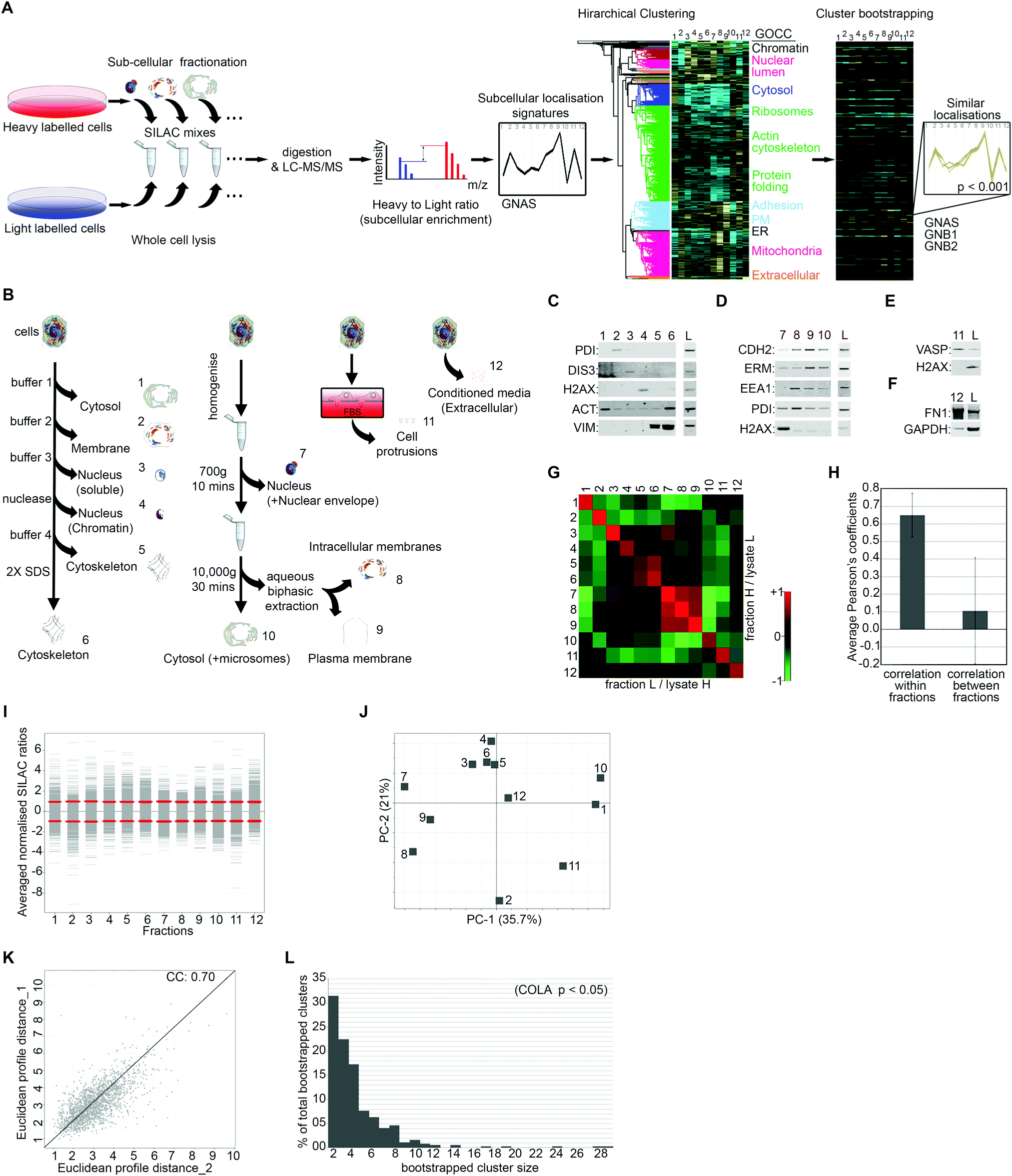 | ||
| Fig. 1 Proteomics-based profiling of colocalisation (COLA) to reveal functional associations. (A) Outline of methodology. SILAC heavy or light labelled cells were subjected to subcellular fractionation then mixed with an equal amount of whole cell lysate from the opposite label for relative quantification. SILAC mixes were digested and analysed by LC-MS/MS. Averaged normalised SILAC ratios for all fractions together create a multi-variate localisation signature for each protein (GNAS was used as example). Signatures were then subjected to unsupervised hierarchical clustering with Euclidean average linkage. Bootstrapping was used to reveal clustering matches with high confidence (in color) from the rest (blacked out). GNAS, GNB1, and GNB2 which are known to constitute a complex are shown as example of a bootstrapped cluster. (B) Outline of the subcellular fractionations. Four independent fractionations procedures were used: (1) serial solubilisation of cellular proteins (fractions 1 to 6), (2) serial centrifugation combined with aqueous biphasic extraction which separates plasma membrane from internal membranes (fractions 7 to 10), (3) separation of actin-rich cellular protrusions using micro-porous transwell filters (fraction 11), (4) separation of the extracellular/secreted proteins by collecting conditioned media (fraction 12). (C) Validation of serial solubilisation method (fractions 1–6) by western blotting: PDI, ER membrane protein; DIS3, soluble nuclear protein; H2AX, nucleosome constituent; actin (ACT) and vimentin (VIM), cytoskeletal proteins; L = matching whole cell lysate control. (D) Validation of serial centrifugation method (fractions 7–10) by western blotting: N-cadherin (CHD2) and ezrin/radixin/moesin proteins (ERM), plasma membrane; early endosomal antigen-1 (EEA1), endosomal; PDI, ER membrane protein; H2AX, nucleosome constituent; L = matching whole cell lysate control. (E) Validation of protrusion purification method (fraction 11) by western blotting: VASP, protrusion; H2AX, nuclear; L = matching cell-body lysate control. (F) Validation of conditioned media collection method (fraction 12) by western blotting: fibronectin-1 (FN1), secreted; GAPDH, intracellular; L = matching whole cell lysate control. (G) Heat map of Pearson correlation coefficients between the two SILAC replicate series of fractionations with switched labelling. Cells were fractionated in duplicate with switching the labels. Collected fraction mixes have high similarity with their corresponding replicate, but low similarity with other fractions. (H) Plotted averaged Pearson's correlation coefficients within replicate fractions versus averaged Pearson's correlation coefficients between different fractions. While a high degree of similarity exists within replicate fractions suggestive of high reproducibility, similarity between different fractions is very low, indicating that each fraction is likely providing unique information. (I) Distribution of SILAC ratios for each fraction (averaged from two replicates). Red lines mark the standard deviations for each fraction. (J) Principle component analysis of subcellular fractions. PC1 and 2 represent over 50% of all data variation. No single fraction contributes towards the overall variation disproportionately. (K) Analysis of the reproducibility of the overall fractionation signatures between two biological replicates. Euclidean distances between each protein signatures from two reciprocally SILAC labelled COLA fractionations were calculated and plotted against each other, showing a highly significant correlation (p < 1.0 × 10⁻¹⁵). The Pearson correlation coefficient (CC) is displayed on the graph. (L) Graph of percentage of total bootstrapped clusters (p < 0.05) vs. the number of proteins per cluster. The majority of clusters are constituted of 2–4 proteins, yet very large clusters are still detectable by COLA. | ||
To maximise acquisition of novel, digitised, information on subcellular protein distributions which would be suitable for hierarchical clustering, we used four parallel independent fractionation procedures with highly distinct individual fractions (Fig. 1B). The majority of subcellular fractions came from two main fractionation procedures, one based on serial solubilisation by using successive solubilising buffers, and the other based on serial centrifugation (Fig. 1B). Both of these procedures are fast, reproducible, require little optimisation, and cover major subcellular compartments. To further expand on subcellular information, we also collected two additional independent fractions, the actin-rich cellular protrusions, and the extracellular compartment (Fig. 1B). Protrusions are purified using transwell based physical separation of cell protrusions from the cell-body,15 and the extracellular compartment is collected by removing and concentrating conditioned media (Fig. 1B). Overall, we identified 4950 proteins from human Retinal Pigment Epithelial (RPE) cells, out of which 1886 had a full subcellular localisation profile with no missing values (Dataset S1, ESI†). The quality of fractionations was examined by western blotting for markers of specific fractions (Fig. 1C–F), as well as category enrichment analysis using the Gene Ontology Cellular Compartment (GOCC) database (Table 1 and Dataset S2, ESI†). For assessing the reproducibility of fractionations, we determined Pearson's correlation coefficients across all fraction replicates. While correlation coefficient within fraction replicates was on average 0.65, suggestive of good reproducibility of fractionations, coefficients between different fractions was only 0.1 on average (Fig. 1G and H), indicating that fractions provide unique information towards the localisation signatures. The distribution and variance of different fractions were comparable (Fig. 1I), and importantly, no single fraction contributed disproportionately to the overall variance (Fig. 1J), ruling out potential bias towards a specific compartment in later downstream analysis. The correlation between the overall subcellular localisation signatures, across two independent biological replicates was calculated to be 0.70 (Fig. 1K).
| Fraction | Significantly enriched GOCC terms (FDR < 0.02) |
|---|---|
| 1 | Cytosol; intracellular |
| 2 | Membrane part; integral component of plasma-membrane; organelle membrane |
| 3 | Nuclear part; nucleoplasm part; transcription factor complex; chromatin remodelling complex; chromatin |
| 4 | Nuclear part; protein–DNA complex; nucleosome; chromosome; nuclear chromosome part; nuclear body |
| 5 | Intermediate filament; nuclear membrane; nucleolus |
| 6 | Intermediate filament; nuclear membrane; nucleolus |
| 7 | Protein–DNA complex; chromatin remodelling complex; nucleoid; organelle part; membrane part |
| 8 | Organelle membrane; membrane enclosed lumen; respiratory chain complex |
| 9 | Plasma membrane; cell junction; coated pit; endosome membrane; membrane part; protein–DNA complex |
| 10 | Cytosolic small ribosomal subunit; cytosolic large ribosomal subunit; proteosome complex; MCM complex |
| 11 | Actin cytoskeleton; ruffle; cell projection; cell junction; adherens junction; synapse; plasma membrane |
| 12 | Extracellular space; extracellular matrix; basement membrane; secretory granule lumen |
To detect proteins that have significantly similar localisation signatures, and therefore are expected to functionally interact, we used hierarchical clustering (Fig. 1A). Hierarchical clustering is ideal for multi-variate assessment of functional interactions as it matches proteins into discrete functional units.3 However, a common shortcoming of standard hierarchical clustering is sensitivity to samples order and variation in clustering results depending on sample inclusion.22 To ensure the significance and robustness of our clustering to permutations, we performed bootstrapped clustering to reveal groups of proteins that group together with high confidence, thus are likely to be truly co-localising (Fig. 1A). We used three different bootstrapping stringency cut-offs of p-value <0.05, 0.01, or 0.001, revealing 365, 271, or 101 bootstrapped clusters (Dataset S3, ESI†), which correspond to 4415, 3087, or 1487 pair-wise co-localisations, respectively (Dataset S4, ESI†). While over 50% of identified bootstrapped clusters contain only 2 or 3 proteins, clusters of 10 or more proteins were also detected (Fig. 1L), suggesting that COLA can detect both small and large complexes.
To verify that COLA predicts real interactions, we assessed its performance in detecting known interactions using three major mammalian functional interaction databases as reference: (1) CORUM, a highly curated database of mammalian protein complexes,25 (2) STRING, a larger database of both physical and functional associations.23 (3) Pathway Commons, a comprehensive collection of functional and physical interactions integrated from multiple publicly available databases.24 We quantified the proportion of co-localising proteins in our method that appear as known functional interactors in each database (Dataset S4, ESI†). Over than half of the COLA identified interactions are annotated as known interactions based on the Pathway Commons database – the largest collection of functional protein interactions (Fig. 2A). Moreover, around 1 in five of COLA interactions are annotated as known in STRING database (Fig. 2B), and a similar percentage of overlap with CORUM interaction database was also detected (Fig. 2C). All of these degrees of overlap are statistically highly significant (p-value <1 × 10−300). For comparison, we also evaluated the performance of two published large-scale studies which used different approaches to map human protein–protein interactions as a proxy for functional associations: (1) Rolland et al., which used Y2H screening,6 and (2) Kristensen et al., which used size-exclusion chromatography coupled with proteomics (SEC-MS).12 Although both studies significantly detected known interactions, they were both consistently outperformed by COLA in every database comparison (Fig. 2A–C). Interestingly, the overlap between each of these three approaches was little despite the significant degree of overlap with the reference databases, suggesting that each method must be revealing complementary information with regards to functional associations (Fig. 2D). These results demonstrate that significant similarity in protein localisation signatures is strongly reflective of a functional interaction, and that COLA outperforms Y2H and SEC-MS methods in revealing functional interactions.
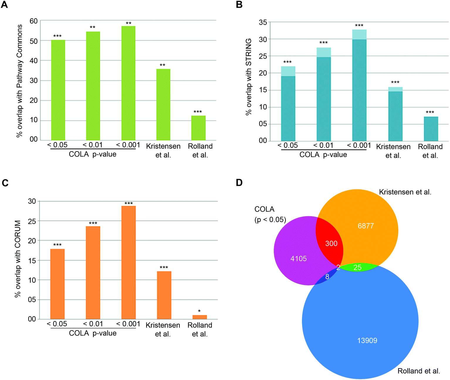 | ||
| Fig. 2 COLA reveals known functional associations and outperforms two current global interactome analysis studies. (A) Percentage of overlap with Pathway Commons between the identified interactions in each bootstrap significance setting, vs. in Kristensen et al.,12vs. in Rolland et al.,6P***: fisher's exact test p < 1 × 10−300; **: fisher's exact test p < 2 × 10−150; *: fisher's exact test p < 1 × 10−75. (B) As in (A) but for overlap with STRING (darker blue indicates physical interactions only). (C) As in (A) but for overlap with CORUM. (D) Venn diagram of the overlap between binary protein–protein interactions revealed COLA versus Kristensen et al., size-exclusion chromatography profiling12 and Rolland et al., Y2H screening.6 Only 2 interactions are shared across the three methods. | ||
Analysis of interactome dynamics by iCOLA
Next, we optimised COLA for analysis of interactome dynamics. A key factor for revealing the dynamics of protein interaction networks is the ability to reliably multiply interactome analyses across several conditions. Thus, high reproducibility along with short analysis times are two crucial criteria for any method designed for analysis of interactome dynamics. The SILAC based COLA method requires a single mass spectrometry run for every fraction/lysate SILAC mix. This equates to a total of 24 runs (2 × 12 reciprocally labelled fraction/lysate mixes) for every analysis, which translates into a total mass spectrometry run time of around 5 days, using our LC-MS/MS settings. To reduce the number of mass spectrometry runs required in order to allow rapid analysis of interactomes across multiple conditions, we developed a modified version of our method (iCOLA), utilising Tandem Mass Tagging (TMT) isobaric labelling which allows mixing and quantification of up to 10 different samples in a single mass spectrometry run.29 To have all the fractions analysed in a single TMT run, we modified our fractionation procedure to have a total of 9 fractions plus 1 whole cell lysate (Fig. 3A). We focused on serial solubilisation and serial centrifugation procedures which provide the bulk of subcellular coverage, and also mixed the two cytoskeletal fractions from serial solubilisation protocol, which had the highest degree of similarity (Fig. 1J), into one fraction (Fig. 3A). Co-localisations were identified as before by determining significant similarities between subcellular localisation signatures using bootstrapped clustering (Fig. 3A). We applied iCOLA to analyse co-localisations in A375P melanoma cells.30 Overall, we identified 2276 proteins, complete subcellular localisation profiles of 1846 of which were defined across all fractions in A375P cells (Dataset S5, ESI†). At the bootstrap cut-off of p-value <0.05, a total of 357 bootstrap clusters were revealed (Dataset S6, ESI†), corresponding to 4916 pair-wise co-localisations (Dataset S7, ESI†). Similar to the SILAC based COLA, the majority of iCOLA identified bootstrapped clusters contained only 2 or 3 proteins, but clusters of 10 or more proteins were also detected (Fig. 3B), suggesting that iCOLA performs comparably to the SILAC based COLA in detecting both small and large complexes. To assess iCOLA's reproducibility, we determined Pearson's correlation coefficients across all fraction replicates as before. Correlation coefficient within fraction replicates was on average 0.92, which is better than COLA, while coefficients between different fractions was on average 0.08 (Fig. 3C and D). In addition, the correlation between the overall fractionation signatures across two independent biological replicates was calculated to be 0.85 (Fig. 3E), which is also better than that of COLA. The improved reproducibility of iCOLA is likely due to the fact that protein quantifications are derived from the same peptides in every fraction, as every identified TMT labelled peptide returns a quantification value for each fraction. In contrast, the same protein can be quantified through different SILAC labelled peptides in each fraction/lysate mix of COLA, thus increasing the likelihood of noise.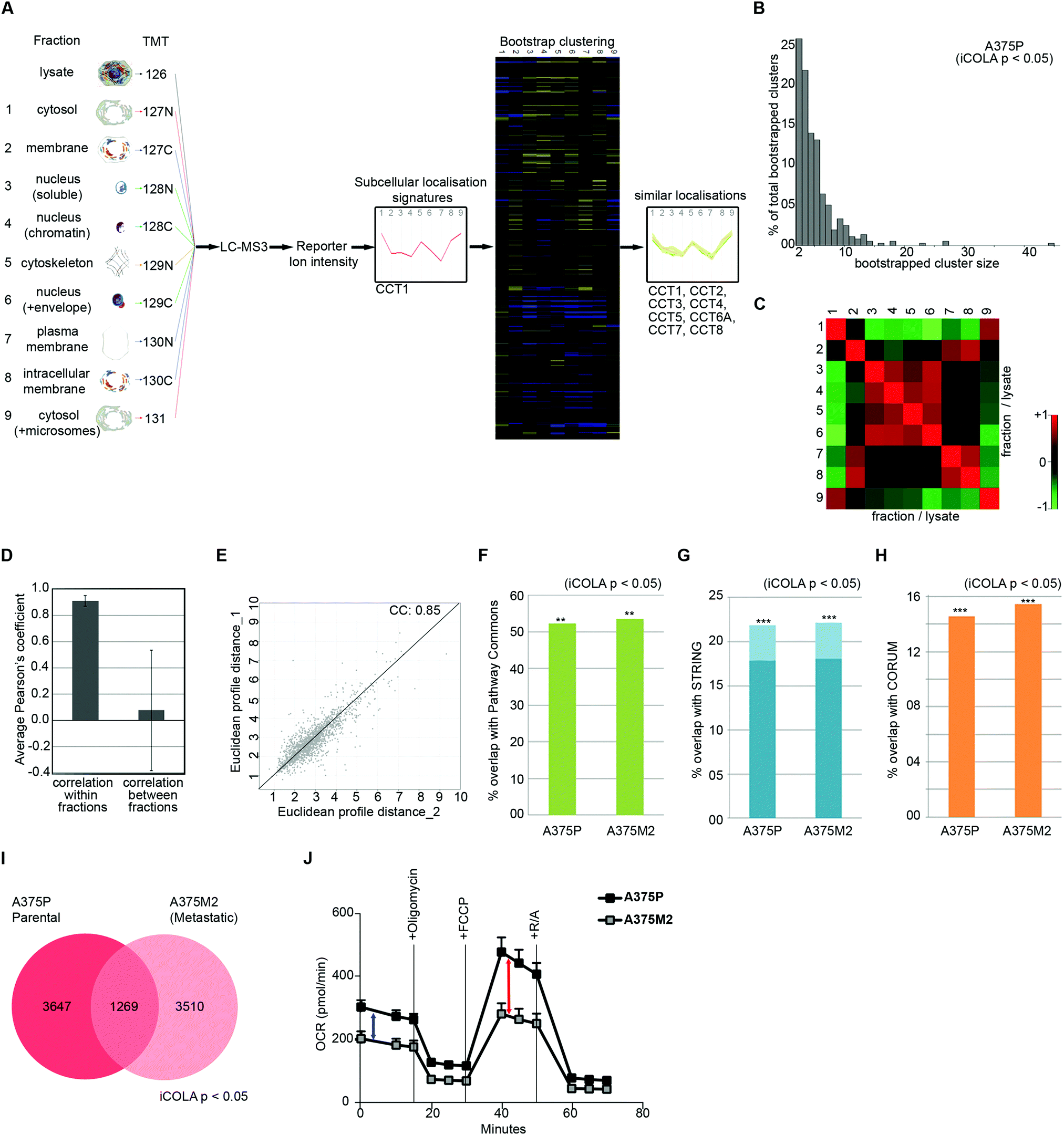 | ||
| Fig. 3 Analysis of interactome dynamics by iCOLA. (A) Outline of the iCOLA methodology. 9 fractions from serial solubilisation and serial centrifugation protocols, along with a 2% SDS solubilised whole cell lysate total control, were digested and isobarically labelled using TMT 10-plex kit as indicated. The labelled peptides were then pooled together and analysed by LC-MS3. Averaged normalised fraction/lysate ratios for every fraction were used to create a multi-variate subcellular localisation signature for each protein (T-complex protein 1 subunit alpha was used as example here). Signatures were then subjected to unsupervised hierarchical clustering with Euclidean average linkage and bootstrapping was used to reveal clustering matches with high confidence (in color) from the rest (blacked out). All members of the TCP1 chaperonin ring complex (CCT1 to 8) are detected as significant interactors of CCT1, and are shown as an example of a bootstrapped cluster. (B) Graph of percentage of total bootstrapped clusters (p < 0.05) vs. the number of proteins per cluster from iCOLA analysis of A375P cells. The majority of clusters are constituted of 2–4 proteins, yet very large clusters are still detectable by iCOLA. (C) Heat map of Pearson correlation coefficients between the two replicate iCOLA series of fractionations. Cells were fractionated in duplicate. Collected fractions show high similarity with their corresponding replicate, but low similarity with other fractions. (D) Plotted averaged Pearson's correlation coefficients within replicate fractions versus averaged Pearson's correlation coefficients between different fractions. While a high degree of similarity exists within replicate iCOLA fractions suggestive of high reproducibility, similarity between different fractions is very low, indicating that each fraction is likely providing unique information. (E) Analysis of the reproducibility of the overall localisation signatures between two biological replicate iCOLA experiments. Euclidean distances between the signatures from two independent iCOLA fractionations experiments in A375P cells were calculated and plotted against each other, showing a highly significant correlation (p < 1.0 × 10⁻¹⁵). The Pearson correlation coefficient (CC) is displayed on the graph. (F) Comparison of the percentage of known interactions according to Pathway Commons that were detected in A375P and A375M2 cells (p < 0.05). Percentage of overlap with Pathway Commons was very similar in A375P and A375M2 cells, and comparable to SILAC based COLA (Fig. 2A). ***: fisher's exact test p < 1 × 10−300; **: fisher's exact test p < 2 × 10−200. (G) Comparison of the percentage of known interactions according to STRING that were detected in A375P and A375M2 cells (p < 0.05). Light blue bars shows all STRING interactions. Dark blue bars show only physical interactions. Percentage of overlap with STRING was very similar in A375P and A375M2 cells, and comparable to SILAC based COLA (Fig. 2B). ***: fisher's exact test p < 1 × 10−300; **: fisher's exact test p < 2× 10−200. (H) Comparison of the percentage of known interactions according to CORUM that were detected in A375P and A375M2 cells (p < 0.05). Percentage of overlap with CORUM was very similar in A375P and A375M2 cells, and comparable to SILAC based COLA (Fig. 2C). ***: fisher's exact test p < 1 × 10−300; **: fisher's exact test p < 2 × 10−200. (I) Venn diagram of the overlap between binary protein–protein interactions detected in A375P and A375M2 cells (bootstrap cut off = 0.05). A core of 1269 interactions were conserved between the two isogenic cell lines, while over 3000 unique interactions were detected in each cell-line. (J) Analysis of mitochondrial respiratory flux in A375P and A375M2 cells. Oxygen consumption (OCR) was measured in real-time, with serial addition of oligomycin to inhibit ATP synthase, FCCP to uncouple oxygen consumption from ATP production, and rotenone/antimycin (R/A) to completely inhibit electron transport chain, at indicated timepoints. Values were normalised to total seeded cell numbers. A375P show a significantly higher basal mitochondrial respiration (blue arrow), as well as a higher maximal mitochondrial respiratory capacity (red arrow), while levels of non-mitochondrial oxygen consumption measured after R/A addition (three ending time points) are equal between both cells. | ||
Next, we applied iCOLA to reveal interactome differences between our previously analysed A375P cells, which are weakly metastatic, to their highly metastatic isogenic derivative, the A375M2 cells.30 We identified 1442 proteins with complete subcellular localisation profiles in A375M2 cells (Dataset S8, ESI†). At the bootstrap cut-off of p-value <0.05, a total of 279 bootstrap clusters were revealed for A375M2 cells, (Dataset S9, ESI†), corresponding to 4779 pair-wise co-localisations (Dataset S10, ESI†). First, to test whether the performance of iCOLA is similar to COLA in terms of identifying true functional interactions in both cell-types, we assessed the overlap of the identified co-localisations with CORUM, STRING, and Pathway Commons interaction databases, as before (Datasets S7 and S10, ESI†). A highly significant proportion of the revealed co-localisations were amongst known functional interactors in both A375P and A375M2 cells (Fig. 3F–H), with the degree of overlap being comparable to that of the SILAC based COLA method, suggesting that reducing the number of fractions from 12 to 9 does not significantly affected the ability of our approach to reveal true interactions. Next, we assessed the degree of overlap between the interactomes of the two cell-lines. 1269 of the interactions identified in total were seen in both A375P and A375M2 cells, whilst more than 3000 interactions were detected in only one cell-type (Fig. 3I). Category enrichment analysis revealed that most conserved interactions belonged to core cellular complexes such as the nucleosome, chaperonin complex, and the ribosome, suggesting that these core interactions do not change much across the two cell-types (Dataset S11, ESI†). In contrast, mitochondrial protein complexes were significantly enriched amongst proteins with changing interactions (Table 2 and Dataset S11, ESI†), suggestive of a substantial rewiring of the mitochondrial interactome between the two cell types. As a result, we hypothesized that mitochondrial activity is likely to be significantly altered between the two cell types. Accordingly, both basal and spare mitochondrial respiratory capacity was significantly reduced in A375M2 cells compared to A375P cells (Fig. 3J). Collectively, these results demonstrate that iCOLA can be used for comparison of functional interactomes between different conditions, and that variations between interactomes can inform on functional differences between different cellular settings.
| Category database | Category name |
|---|---|
| Corum | 55S ribosome, mitochondrial |
| Keywords | Ligase |
| GSEA | RESPIRATORY_ELECTRON_TRANSPORT |
| GOBP | Coenzyme metabolic process |
| GOBP | Cofactor metabolic process |
| GOCC | Mitochondrial matrix |
| Keywords | Mitochondrion |
| Keywords | Transitpeptide |
| GOCC | Mitochondrial part |
| GSEA | TCA_CYCLE_AND_RESPIRATORY_ELECTRON_TRANSPORT |
| GSEA | WONG_MITOCHONDRIA_GENE_MODULE |
| GSEA | MOOTHA_MITOCHONDRIA |
| GOBP | Oxidation–reduction process |
| GSEA | MOOTHA_HUMAN_MITODB_6_2002 |
| GSEA | MITOCHONDRION |
| GOCC | Mitochondrion |
| GSEA | LEE_BMP2_TARGETS_DN |
| GOBP | Small molecule metabolic process |
COLA is sensitive and specific
We next assessed the quality of COLA and iCOLA for interactome mapping, by calculating four critical parameters that measure key attributes of a given global protein–protein interaction detection method, as outlined by Vidal and colleagues.27 These four parameters are completeness, False Positive Rate (FPR), Sensitivity (Recall), and Precision. Completeness is the measure of the percentage of total possible interactions covered by an assay. FPR is the probability of reporting a false interaction. Sensitivity is the measure of the percentage of all true interactions that are reported by the assay. Finally, Precision measures the percentage of reported interactions which are true. Assay completeness directly corresponds to the number of investigated proteins (i.e. in our case proteins which were identified and quantified in all fractions). Assuming that there are ∼22500 proteins in human genome, the total size of the possible interactome is equal to 22500 × 22500/2 = 253125000. In COLA, we identified 1886 proteins, meaning that 1886 × 1886/2 = 1778498 possible interactions were tested, which is ∼1.4% of the total possible interactome space. This compares similarly with Kristensen et al., SEC-MS method for mining of interactions,12 but is less than most Y2H screens, which cover a larger ORFome space.6,27
In a binary interactome analysis, assuming the null-hypothesis (H0) equates to proteins A and B not interacting (false interaction), and alternative hypothesis (H1) to A and B interacting (true interaction), various types of possible interactions can be defined, which are listed in (Table 3).
| H(0) is correct | H(1) is correct | Sum | |
|---|---|---|---|
| Note: V + S = R; U + T = R′; V + U = M′; S + T = M; M′ + M = A. | |||
| Reported interactions | V (false positives) | S (true positives) | R |
| Unreported interactions | U (true negatives) | T (false negatives) | R′ |
| Sum | M′ (total false interactions) | M (total interactions) | A |
Assuming that the null hypothesis (H0) in a protein–protein interaction detection assay is no interaction, and the alternative hypothesis (H1) is existence of an interaction, a global binary interactome analysis method can report two types of interaction: true positive (S), and false positive (V). The total number of reported interactions (R) is therefore the sum of S and V. Conversely, the unreported interactions consist of true (U) and false negatives (T), with the total number of unreported interactions (R′) consisted of the sum of U and T. In addition, all true interactions in the interactome space (M), whether reported or not by the method, can be defined as the sum of S and T. Similarly, all false interactions in the interactome space (M′), whether reported or not, can be defined as the sum of V and U. Finally the total size of the hypothetical interactome space (A) can be defined as the sums of M and M′, or R and R′.
Accordingly, FPR, Sensitivity, and Precision can be defined as a function of these types of interactions:
• Sensitivity = S/M
• FPR = V/M′
• Precision = S/R
CORUM is a highly curated database of well-known protein interactions, which can be regarded as almost ‘True’.25 To estimate Sensitivity, we can therefore simply calculate the proportion of CORUM interactions that were reported by COLA, for the list of identified input proteins. COLA and iCOLA have a Sensitivity of ∼3% to 6%, depending on the bootstrapping cut-off (Fig. 4A). In comparison, based on CORUM, Kristensen et al.'s SEC-MS method12 and Rolland et al.'s Y2H study6 had Sensitivities of ∼8% and ∼2%, respectively (Fig. 4A). Thus, COLA is roughly similar in terms of its Sensitivity to both of these existing methods.
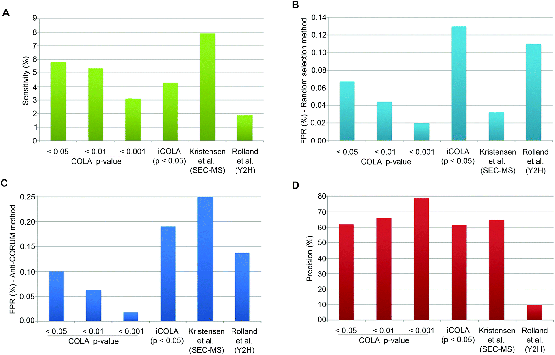 | ||
| Fig. 4 Analysis of Sensitivity, FPR, and Precision for COLA and iCOLA. (A) Comparison of Sensitivity, also termed Recall, between COLA (at bootstrapping cut off p-values of 0.05, 0.01, and 0.001), iCOLA (at cut off p-value of 0.05), Kristensen et al.'s SEC-MS method,12 and Rolland et al.'s Y2H screen.6 Sensitivity was defined as percentage of interactions present in CORUM that were identified by each method. (B) Comparison of FPR between COLA (at bootstrapping cut off p-values of 0.05, 0.01, and 0.001), iCOLA (at cut off p-value of 0.05), Kristensen et al.'s SEC-MS method,12 and Rolland et al.'s Y2H screen.6 FPR was defined as the percentage of interactions from a list of randomly selected 200 binary interactions not previously reported in any database (see Materials and methods) which were identified by each method. The sampling of 200 unknown interactions was performed 1000 times, and percentage values were averaged and displayed. (C) An alternative comparison of FPR, between COLA (at bootstrapping cut off p-values of 0.05, 0.01, and 0.001), iCOLA (at cut off p-value of 0.05), Kristensen et al.'s SEC-MS method,12 and Rolland et al.'s Y2H screen.6 FPR was defined as percentage of interactions present in the anti-CORUM dataset (see Materials and methods) that were identified by each method. (D) Comparison of Precision between COLA (at bootstrapping cut off p-values of 0.05, 0.01, and 0.001), iCOLA (at cut off p-value of 0.05), Kristensen et al.'s SEC-MS method,12 and Rolland et al.'s Y2H screen.6 As the total size of the hypothetical interactome space (A), as well as the total number of reported (R) and unreported (R′) interactions are known for each method, the measures of Sensitivity (S/M) and FPR (V/M′) can be used to estimate S, M, M′, T, and U values. Precision was then calculated as S/R, and displayed as a percentage value. COLA, and iCOLA have comparable or slightly better Precision than Kristensen et al.'s SEC-MS method, but both vastly outperform Rolland et al.'s Y2H. | ||
Estimation of FPR is somewhat tricky as no reference database of false interactions (protein–protein interactions that definitely do not occur) exists. To circumvent this problem, we used two alternative approaches to generate lists of likely to be false interactions. In the first approach, we simply made a list of 200 randomly generated interactions which were not reported to interact with one another in any known protein interaction database (thus at least enriched in false interactions compared to the background), and calculated the percentage of these interactions that were detected by COLA and iCOLA. This method has been utilised by Vidal and colleagues to estimate the FPR of various Y2H screens, which were reported at 0.5 to 2%.27 The downside of such an approach is potential errors that could be introduced due to random sampling. To counteract such bias, we repeated our sampling of the 200 unreported interactions a thousand times, calculating the FPR for all of them and averaging the resulting values. Based on this approach, COLA and iCOLA were estimated to have FPR of 0.02 to ∼0.1% depending on the bootstrapping cut-off (Fig. 4B). Using the same estimation strategy, FPR of Kristensen et al.'s SEC-MS was calculated to be ∼0.03% while Rolland et al.'s Y2H had an FPR of ∼0.1% (Fig. 4B).
A major issue with the aforementioned strategy is that many unreported interactions maybe yet undiscovered true interactions as opposed to false ones, and this is particularly likely if a given protein is not well studied in terms of its interactions, thus not well annotated in interaction databases. So as an alternative approach to generate a library of likely to be false interactions, we used a method based on a strategy recently proposed by Foster and colleagues.31 In this method, it is reasoned that as CORUM is a highly curated database of well-known protein interactions, if a given protein is already annotated in CORUM, it is likely that its interactions are better defined, so if two such CORUM annotated proteins are not reported to interact with each other, they are more likely to be false interactors. Based on this rationale, we created a library of possible false interactions, which we named anti-CORUM (proteins which are listed in CORUM but not known to interact), and used it to estimate the FPR by calculating the percentage of these anti-CORUM interactions that were identified by COLA and iCOLA. Depending on the bootstrapping cut-off stringency, COLA and iCOLA's FPR was estimated at 0.02 to ∼0.19% (Fig. 4C). Using the same strategy, the FPR for Kristensen et al.'s SEC-MS was ∼0.25% while Rolland et al.'s Y2H had an FPR of ∼0.14% (Fig. 4C). Thus, the FPR of COLA and iCOLA are better than that of SEC-MS, and better or comparable with Y2H, depending on the bootstrapping cut-off.
Finally, using the anti-CORUM estimated Sensitivity and FPR, we estimated V, S, U, and T values (Table 3), which allowed calculation of Precision for COLA and iCOLA. Depending on the bootstrapping cut off stringency, COLA and iCOLA's Precision were calculated at ∼61 to 79%. In comparison, SEC-MS had a Precision of ∼65%, while Y2H Precision was ∼10% (Fig. 4D). Thus, while COLA and iCOLA have comparable or slightly better Precision than Kristensen et al.'s SEC-MS, they vastly outperform Rolland et al.'s Y2H screen. Collectively, these results demonstrate that significant similarity in protein localisation signatures can be confidently used to reveal interactions, and that COLA and iCOLA vastly outperform Y2H in terms of Precision, which is the key measure of assay specificity.
Discussion
Robust methods that reveal dynamics of functional interactions between proteins on a global scale are crucial for system level understanding of cellular processes. Quantitative proteomics in conjugation with biochemical fractionation by chromatography,11–13 is a recent approach that attempts to address the issue of assessing interactome dynamics, but is limited to soluble proteins and can miss on more transient interactions. Here, we present COLA, a global proteomics based strategy that reveals significant co-localisation as a proxy for functional associations. Our approach is not limited to soluble protein complexes and does not solely report biochemical associations. Instead, it robustly matches interacting proteins based on similarity in their multi-dimensional subcellular localisation signatures. In addition, COLA requires significantly less number of proteomics runs per experiment than the previously published chromatography based methods.11,12 All subcellular fractionations can be performed in a single day, with proteomics sample preparation and digestion taking two additional days. If the iCOLA approach is used, mass spectrometry runs will only take a few hours, meaning that the whole analysis can be completed in less than a week, including data processing and clustering. This makes iCOLA much faster than any previously published global protein–protein interaction analysis method, and ideal for studying global interactome dynamics. As a proof of principle, we here used iCOLA for such analysis, comparing the interactomes of weakly and highly metastatic isogenic melanoma cells. Our analysis revealed a significant rewiring of the mitochondrial interactome (Table 2), and in line with this observation, the mitochondrial respiratory activity was found to be significantly altered between the two cell-lines (Fig. 3J). The functional significance of this metabolic change with regards to the metastatic potential of the cells remains to be determined.Although subcellular localisation of proteins has been studied by proteomics before,28,32–37 the focus of most of these studies has been on assigning proteins to different organelles rather than revealing protein–protein interactions. Comprehensive subcellular localisation profiling to reveal interactions has been performed by microscopy, using high-throughput fluorescent tagging in combination with high-content imaging.14 Also, a related non-microscopy based method known as proximity based biotin labelling functions by tagging bait proteins with a promiscuous biotin ligase, which then biotinylates any closely localising proteins in vivo, allowing their subsequent affinity purification and identification of by mass spectrometry. However, similar to Y2H or AP-MS, both these approaches suffer from the labour intensive need to tag every target protein in a cell-type of interest, and are prone to potential artefacts caused by the addition of a fluorescent or a biotin ligase tag. In contrast, COLA can be applied to any cell-type, and in a fraction of the time required for other methods. Fractionations, sample preparations, and computational methods used in COLA are all well established, making it a readily available tool to a wide range of biologist across diverse fields. Finally, our benchmarking shows that COLA and iCOLA compare favourably with some of the existing methods of interactome mining in terms of the quality of their interactome data. With regards to their Sensitivity, COLA and iCOLA are comparable with SEC-MS, and perform better than Y2H (Fig. 4A). More importantly, COLA and iCOLA perform comparable or better than SEC-MS in terms of their Precision, while greatly outperforming Y2H (Fig. 4D). COLA and iCOLA therefore compare favourably with some of the existing global methods for reliable unbiased mining of interactomes.
Conclusions
Subcellular localisation of a protein is an important determinant of the functional interactions it can form in a given cellular context. COLA uses a quantitative proteomics approach to assess subcellular localisation of proteins on a global scale, and then matches proteins with highly similar subcellular localisation patterns using multi-variate localisation signatures. The rapid nature of COLA, its applicability to almost any cell-type, as well as its accuracy and ease of use for revealing functional interactions on a global scale, renders it highly suitable for assessing functional interactomes across multiple conditions and treatments. We predict that such an approach is likely to have a decisive impact on systems level analysis of functional interactions, as methods to rapidly reveal interactome dynamics on a global scale are desperately needed.Author contributions
The study was envisaged by FKM. Experiments were designed by FKM, CB, and CJM. FKM wrote the manuscript. HZS performed all bioinformatics analyses. SK & RRM assisted with subcellular fractionations. AP assisted with sample preparation of SILAC based COLA samples. CJT and CJ performed sample preparation, TMT labelling, and LC-MS3 analyses of iCOLA samples. SA and GP performed the analysis of mitochondrial flux. All other experiments were performed by FKM.Conflict of interest
Authors declare no conflict of interest.Acknowledgements
We would like to thank ICR's and Cancer Research UK Manchester Institute's proteomics core facilities for mass spectrometry runs. We would also like to thank all Marshall Lab members for their comments and useful discussions. FKM, SK, RRM, AP, and CJM were funded by Cancer Research UK (grant numbers C107/A12057, C107/A10433 & C107/A16512). CJM was a Gibb Life Fellow of CRUK. HZS and CB were funded by BBSRC project grant BB/J017183/1 and CRUK Programme Foundation Award (C37275/A20146). CJT is funded by a Sir Henry Wellcome Postdoctoral Fellowship (098847/Z/12/Z). CJ is funded by a Cancer Research UK Career Establishment Award (C37293/A12905) and a Cancer Research UK Institute Award (A19258).References
- P. Liberali, B. Snijder and L. Pelkmans, Nat. Rev. Genet., 2015, 16, 18–32 CrossRef CAS PubMed.
- C. Bakal, J. Aach, G. Church and N. Perrimon, Science, 2007, 316, 1753–1756 CrossRef CAS PubMed.
- B. Snijder, P. Liberali, M. Frechin, T. Stoeger and L. Pelkmans, Nat. Methods, 2013, 10, 1089–1092 CrossRef CAS PubMed.
- S. Oliver, Nature, 2000, 403, 601–603 CrossRef CAS PubMed.
- K. Tarassov, V. Messier, C. R. Landry, S. Radinovic, M. M. Serna Molina, I. Shames, Y. Malitskaya, J. Vogel, H. Bussey and S. W. Michnick, Science, 2008, 320, 1465–1470 CrossRef CAS PubMed.
- T. Rolland, M. Tasan, B. Charloteaux, S. J. Pevzner, Q. Zhong, N. Sahni, S. Yi, I. Lemmens, C. Fontanillo, R. Mosca, A. Kamburov, S. D. Ghiassian, X. Yang, L. Ghamsari, D. Balcha, B. E. Begg, P. Braun, M. Brehme, M. P. Broly, A. R. Carvunis, D. Convery-Zupan, R. Corominas, J. Coulombe-Huntington, E. Dann, M. Dreze, A. Dricot, C. Fan, E. Franzosa, F. Gebreab, B. J. Gutierrez, M. F. Hardy, M. Jin, S. Kang, R. Kiros, G. N. Lin, K. Luck, A. MacWilliams, J. Menche, R. R. Murray, A. Palagi, M. M. Poulin, X. Rambout, J. Rasla, P. Reichert, V. Romero, E. Ruyssinck, J. M. Sahalie, A. Scholz, A. A. Shah, A. Sharma, Y. Shen, K. Spirohn, S. Tam, A. O. Tejeda, S. A. Trigg, J. C. Twizere, K. Vega, J. Walsh, M. E. Cusick, Y. Xia, A. L. Barabasi, L. M. Iakoucheva, P. Aloy, J. De Las Rivas, J. Tavernier, M. A. Calderwood, D. E. Hill, T. Hao, F. P. Roth and M. Vidal, Cell, 2014, 159, 1212–1226 CrossRef CAS PubMed.
- E. L. Huttlin, L. Ting, R. J. Bruckner, F. Gebreab, M. P. Gygi, J. Szpyt, S. Tam, G. Zarraga, G. Colby, K. Baltier, R. Dong, V. Guarani, L. P. Vaites, A. Ordureau, R. Rad, B. K. Erickson, M. Wuhr, J. Chick, B. Zhai, D. Kolippakkam, J. Mintseris, R. A. Obar, T. Harris, S. Artavanis-Tsakonas, M. E. Sowa, P. De Camilli, J. A. Paulo, J. W. Harper and S. P. Gygi, Cell, 2015, 162, 425–440 CrossRef CAS PubMed.
- M. Y. Hein, N. C. Hubner, I. Poser, J. Cox, N. Nagaraj, Y. Toyoda, I. A. Gak, I. Weisswange, J. Mansfeld, F. Buchholz, A. A. Hyman and M. Mann, Cell, 2015, 163, 712–723 CrossRef CAS PubMed.
- K. J. Roux, D. I. Kim, M. Raida and B. Burke, J. Cell Biol., 2012, 196, 801–810 CAS.
- A. H. Smits and M. Vermeulen, Trends Biotechnol., 2016, 34, 825–834 CrossRef CAS PubMed.
- P. C. Havugimana, G. T. Hart, T. Nepusz, H. Yang, A. L. Turinsky, Z. Li, P. I. Wang, D. R. Boutz, V. Fong, S. Phanse, M. Babu, S. A. Craig, P. Hu, C. Wan, J. Vlasblom, V. U. Dar, A. Bezginov, G. W. Clark, G. C. Wu, S. J. Wodak, E. R. Tillier, A. Paccanaro, E. M. Marcotte and A. Emili, Cell, 2012, 150, 1068–1081 CrossRef CAS PubMed.
- A. R. Kristensen, J. Gsponer and L. J. Foster, Nat. Methods, 2012, 9, 907–909 CrossRef CAS PubMed.
- C. Wan, B. Borgeson, S. Phanse, F. Tu, K. Drew, G. Clark, X. Xiong, O. Kagan, J. Kwan, A. Bezginov, K. Chessman, S. Pal, G. Cromar, O. Papoulas, Z. Ni, D. R. Boutz, S. Stoilova, P. C. Havugimana, X. Guo, R. H. Malty, M. Sarov, J. Greenblatt, M. Babu, W. B. Derry, E. R. Tillier, J. B. Wallingford, J. Parkinson, E. M. Marcotte and A. Emili, Nature, 2015, 525, 339–344 CrossRef CAS PubMed.
- Y. T. Chong, J. L. Koh, H. Friesen, S. K. Duffy, M. J. Cox, A. Moses, J. Moffat, C. Boone and B. J. Andrews, Cell, 2015, 161, 1413–1424 CrossRef CAS PubMed.
- F. K. Mardakheh, A. Paul, S. Kumper, A. Sadok, H. Paterson, A. McCarthy, Y. Yuan and C. J. Marshall, Dev. Cell, 2015, 35, 344–357 CrossRef CAS PubMed.
- J. R. Wisniewski, D. F. Zielinska and M. Mann, Anal. Biochem., 2011, 410, 307–309 CrossRef CAS PubMed.
- G. S. McDowell, A. Gaun and H. Steen, J. Proteome Res., 2013, 12, 3809–3812 CrossRef CAS PubMed.
- L. Ting, R. Rad, S. P. Gygi and W. Haas, Nat. Methods, 2011, 8, 937–940 CrossRef CAS PubMed.
- S. Tyanova, M. Mann and J. Cox, Methods Mol. Biol., 2014, 1188, 351–364 Search PubMed.
- S. Tyanova, T. Temu, P. Sinitcyn, A. Carlson, M. Y. Hein, T. Geiger, M. Mann and J. Cox, Nat. Methods, 2016, 13, 731–740 CrossRef CAS PubMed.
- J. Cox and M. Mann, BMC Bioinf., 2012, 13(Suppl 16), S12 CrossRef CAS PubMed.
- R. Suzuki and H. Shimodaira, Bioinformatics, 2006, 22, 1540–1542 CrossRef CAS PubMed.
- A. Franceschini, D. Szklarczyk, S. Frankild, M. Kuhn, M. Simonovic, A. Roth, J. Lin, P. Minguez, P. Bork, C. von Mering and L. J. Jensen, Nucleic Acids Res., 2013, 41, D808–D815 CrossRef CAS PubMed.
- E. G. Cerami, B. E. Gross, E. Demir, I. Rodchenkov, O. Babur, N. Anwar, N. Schultz, G. D. Bader and C. Sander, Nucleic Acids Res., 2011, 39, D685–D690 CrossRef CAS PubMed.
- A. Ruepp, B. Waegele, M. Lechner, B. Brauner, I. Dunger-Kaltenbach, G. Fobo, G. Frishman, C. Montrone and H. W. Mewes, Nucleic Acids Res., 2010, 38, D497–D501 CrossRef CAS PubMed.
- C. J. Tape, S. Ling, M. Dimitriadi, K. M. McMahon, J. D. Worboys, H. S. Leong, I. C. Norrie, C. J. Miller, G. Poulogiannis, D. A. Lauffenburger and C. Jorgensen, Cell, 2016, 165, 910–920 CrossRef CAS PubMed.
- K. Venkatesan, J. F. Rual, A. Vazquez, U. Stelzl, I. Lemmens, T. Hirozane-Kishikawa, T. Hao, M. Zenkner, X. Xin, K. I. Goh, M. A. Yildirim, N. Simonis, K. Heinzmann, F. Gebreab, J. M. Sahalie, S. Cevik, C. Simon, A. S. de Smet, E. Dann, A. Smolyar, A. Vinayagam, H. Yu, D. Szeto, H. Borick, A. Dricot, N. Klitgord, R. R. Murray, C. Lin, M. Lalowski, J. Timm, K. Rau, C. Boone, P. Braun, M. E. Cusick, F. P. Roth, D. E. Hill, J. Tavernier, E. E. Wanker, A. L. Barabasi and M. Vidal, Nat. Methods, 2009, 6, 83–90 CrossRef CAS PubMed.
- F. M. Boisvert, Y. W. Lam, D. Lamont and A. I. Lamond, Mol. Cell. Proteomics, 2010, 9, 457–470 CAS.
- B. K. Erickson, M. P. Jedrychowski, G. C. McAlister, R. A. Everley, R. Kunz and S. P. Gygi, Anal. Chem., 2015, 87, 1241–1249 CrossRef CAS PubMed.
- E. A. Clark, T. R. Golub, E. S. Lander and R. O. Hynes, Nature, 2000, 406, 532–535 CrossRef CAS PubMed.
- N. E. Scott, L. M. Brown, A. R. Kristensen and L. J. Foster, J. Proteomics, 2015, 118, 112–129 CrossRef CAS PubMed.
- V. K. Mootha, J. Bunkenborg, J. V. Olsen, M. Hjerrild, J. R. Wisniewski, E. Stahl, M. S. Bolouri, H. N. Ray, S. Sihag, M. Kamal, N. Patterson, E. S. Lander and M. Mann, Cell, 2003, 115, 629–640 CrossRef CAS PubMed.
- T. P. Dunkley, R. Watson, J. L. Griffin, P. Dupree and K. S. Lilley, Mol. Cell. Proteomics, 2004, 3, 1128–1134 CAS.
- L. J. Foster, C. L. de Hoog, Y. Zhang, Y. Zhang, X. Xie, V. K. Mootha and M. Mann, Cell, 2006, 125, 187–199 CrossRef CAS PubMed.
- M. W. Trotter, P. G. Sadowski, T. P. Dunkley, A. J. Groen and K. S. Lilley, Proteomics, 2010, 10, 4213–4219 CrossRef CAS PubMed.
- A. Christoforou, C. M. Mulvey, L. M. Breckels, A. Geladaki, T. Hurrell, P. C. Hayward, T. Naake, L. Gatto, R. Viner, A. Martinez Arias and K. S. Lilley, Nat. Commun., 2016, 7, 8992 Search PubMed.
- D. N. Itzhak, S. Tyanova, J. Cox and G. H. Borner, eLife, 2016, 5, e16950 Search PubMed.
Footnotes |
| † Electronic supplementary information (ESI) available. See DOI: 10.1039/c6mb00701e |
| ‡ These authors contributed equally to the work. |
| § Deceased. |
| This journal is © The Royal Society of Chemistry 2017 |